Unified 3D Analytical Models of Surface-Inserted Axial Flux Machines With Odd-/Even-Piece Halbach Arrangements

Youyuan Ni¹, Jinsong Zou¹, Yong Lin¹, and Anbang Wang²

¹School of Electrical Engineering & Automation Hefei University of Technology, Hefei 230009, China
nyy@hfut.edu.cn, 2024110327@mail.hfut.edu.cn, linyong@hfut.edu.cn

²Yangzhou Haitong Electronic Technology Co. Ltd. Yangzhou 225001, China
delsuner@163.com

Submitted On: March 09, 2026
Accepted On: June 15, 2026

ABSTRACT

Considering the 3-dimensional (3D) air-gap fringing field, unified 3D analytical models equivalent to linear machines are proposed for surface-inserted axial flux machines (SIAFMs) with odd-/even-piece Halbach arrangements. The 3D scalar potential governing equations for several regions can be uniquely solved according to Fourier decomposition coefficient matrixes derived from field boundary conditions. Based on this, the electromagnetic parameters can be derived. Predictions indicate that, compared with the non-optimized SIAFMs with three-/four-piece Halbach arrangements, the optimized SIAFMs with three-/four-piece Halbach arrangements exhibit excellent electromagnetic performances. The 3D finite element (FE) and analytical predictions for the SIAFM models are compared.

Keywords: Odd-/even-piece Halbach arrangements, surface-inserted axial flux machine, unified 3D analytical model..

1 INTRODUCTION

Different from the non-optimized radial flux permanent magnet (PM) machines, axial flux machines with PMs have not only smaller volume but also higher torque and power density although they may lead to larger torque ripple [1, 2]. With the progress and development of society, especially extensive use of rare earth materials and improvement of control techniques, more axial flux machines, which are used in fields like electric vehicles, aerospace, and wind power [2, 3, 4], are needed.

A great variety of academic research on surface-mounted axial flux machines (SMAFMs) with PMs is carried out with the aim of improving their performance. Halbach arrangements that not only weaken torque ripple but also gather the magnetic field [4], are used for SMAFMs in [4, 5, 6, 7, 8, 9], and the combination of magnet circumferential displacement with various pole-arc ratios and magnet axial shape design are utilized to reduce pulsating torque in [10]. Surface-inserted axial flux machines (SIAFMs) with different thickness Halbach magnets and soft magnetic materials are proposed in [11]. Axial flux machines combining surface-inserted and surface-mounted magnets are analyzed in [7].

As a numeric solution approach, the 3-dimensional (3D) finite element (FE) analysis takes a long computation time, especially for optimization. In order to reduce the computing time, a few approaches have been presented. An approach with 2-dimensional (2D) scalar potential equivalent to linear motor for SMAFM is proposed in [5, 12, 13]. A 2D analytical model with vector potential is presented for achieving the magnetic field in SMAFMs with Halbach arrangements in [14, 15], and a method with 2D vector potential equivalent to linear machine is proposed in [4, 6, 16, 17, 18]. However, these approaches, except [13, 17], ignore the fringing effect in radial direction, and the methods with correction coefficient proposed in [13, 17] still have a degree of error. Then, 3D scalar potential techniques based on Bessel function in [18, 19, 20] or virtual argument Bessel function in [8, 9, 21] are presented. These 3D techniques can only solve the fields in SMAFMs and have non-negligible errors with the equivalent method in [7]. In addition, an equivalent method with the 3D scalar potential equivalent to linear motors has been proposed in [22, 23, 24, 25], but it cannot be used for SIAFMs. The approach proposed in [26] only applies to surface-inserted radial flux PM machines.

In this paper, unified 3D analytical models are proposed for SIAFMs with odd-/even-piece Halbach arrangements. By means of solving the Fourier decomposition of boundary condition matrix in equivalent linear machines, the field governing equations in different regions are solved. The stator slotting effect is taken into account by Carter’s coefficient. Different from 2D radial flux machines, the air-gap fringing effect for SIAFMs needs to be considered and the air-gap fringing field is analyzed. According to the solved magnetic fields, the electromagnetic performances are obtained. Computation results demonstrate that the optimized pieced Halbach arrangement SIAFMs have better performance than the corresponding non-optimized ones. A comparison of 3D FE and analytical predictions demonstrates that the proposed 3D analytical model is valid.

2 3D PHYSICAL MODEL FOR HALBACH SIAFMS

2.1 Geometrical parameters for Halbach arrangements

Figures 1 (a) and (b) show the design parameters of the odd-/even-piece Halbach arrangements for SIAFMs. For the odd/even-piece Halbach, ${\alpha }_1,\mathrm{\dots }$, and ${\alpha }_{\lambda }$ are the arc ratios of all the magnet pieces. Regardless of odd-or even-piece number, $\alpha$ is the proportion of polar arcs between two rotor teeth, ${\alpha }_0$ is the arc ratio of all the N or S magnets. For both odd- and even-piece Halbach arrangements, the magnetization angles between the axial symmetric axis and the magnetization directions are defined as ${\theta }_1,\mathrm{\dots }$, and ${\theta }_{\lambda +1}$. In particular, for the odd-piece Halbach, ${\theta }_1=0^{\circ }$. If ${\theta }_1$ is equal to zero for the even-piece Halbach, the even-piece Halbach is equivalent to the odd-piece Halbach.

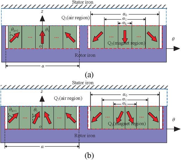
Figure 1 Design parameters of surface-inserted odd-/even-piece Halbach arrangements: (a) odd-piece Halbach and (b) even-piece Halbach.

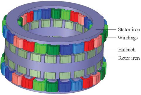
Figure 2 3D structure of SIAFM with three-piece Halbach arrangements.

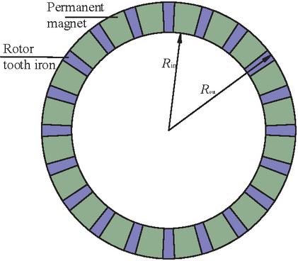
Figure 3 Top view of SIAFM.

Figure 2 clearly exhibits the 3D structure of single rotor and double stator SIAFM with three-piece Halbach arrangements. In the cylindrical coordinate systems, the 3D analytical equations of SIAFM models can be hardly solved. As a consequence, for easy solution of the 3D field distributions in SIAFMs with Halbach arrangements, the cylindrical coordinate system is converted to the spatial Cartesian one. However, due to the difference between inner and outer diameters, the unfolded ring cannot be strictly equivalent to a rectangle. In order to ensure the rigor and accuracy of the equivalent calculation, the PMs can be divided into $n_t$ (an odd number) circular cylinder slices with unequal inner and outer radii but equal differences between inner and outer radii. From inside to outside, the circular cylindrical regions are numbered as $1,\mathrm{\dots },j,\mathrm{\dots }$, and $n_t$. Therefore, the average radius of the $j$-th circular cylinder can be computed as

$$R_j=R_{\mathrm{in}}+(j-1)\frac{R_{\mathrm{out}}-R_{\mathrm{in}}}{n_t}+\frac{1}{2}\frac{R_{\mathrm{out}}-R_{\mathrm{in}}}{n_t},$$

(1)

where $R_{\mathrm{in}}$ and $R_{\mathrm{out}}$ are the inner and outer radii, respectively, as shown in Fig. 3.

2.2 Magnetization parameters for Halbach arrangements

The double Fourier decomposition of magnetization by trigonometric functions are one key point of the analytical model. However, because of the special circumstances of the rotor teeth, polar distance cannot be used as half a cycle of magnetization components. Through the mirror method, the length between the rotor teeth can be considered as half a cycle of the magnetization components. In the spatial Cartesian coordinate system, the three magnetization components in $x$-, $y$-, and $z$-directions for odd-piece Halbach (given three-piece Halbach as an example) between $-l/2$ to $3l/2$ can be expressed as

$\{\begin{array}{cc}{M}_x^j={\displaystyle \frac{B_{re}}{{\mu }_0}}\sin ({\theta }_2)\hfill & -{\displaystyle \frac{{\alpha }_{0}l}{2\alpha }}<x<-{\displaystyle \frac{{\alpha }_{1}l}{2\alpha }}\hfill \\ M_y^j=0\hfill & -{\displaystyle \frac{q{n}_t}{2}}<y<{\displaystyle \frac{q{n}_t}{2}}\hfill \\ M_z^j={\displaystyle \frac{B_{re}}{{\mu }_0}}\cos ({\theta }_2)\hfill & \end{array},$	(5)
$\{\begin{array}{cc}{M}_x^j=0\hfill & -{\displaystyle \frac{{\alpha }_{1}l}{2\alpha }}<x<{\displaystyle \frac{{\alpha }_{1}l}{2\alpha }}\hfill \\ M_y^j=0\hfill & -{\displaystyle \frac{q{n}_t}{2}}<y<{\displaystyle \frac{q{n}_t}{2}}\hfill \\ M_z^j={\displaystyle \frac{B_{re}}{{\mu }_0}}\hfill & \end{array},$	(9)
$\{\begin{array}{cc}{M}_x^j=-{\displaystyle \frac{B_{re}}{{\mu }_0}}\sin ({\theta }_2)\hfill & {\displaystyle \frac{{\alpha }_{1}l}{2\alpha }}<x<{\displaystyle \frac{{\alpha }_{0}l}{2\alpha }}\hfill \\ M_y^j=0\hfill & -{\displaystyle \frac{q{n}_t}{2}}<y<{\displaystyle \frac{q{n}_t}{2}}\hfill \\ M_z^j={\displaystyle \frac{B_{re}}{{\mu }_0}}\cos ({\theta }_2)\hfill & \end{array},$	(13)
$\{\begin{array}{cc}{M}_x^j=-{\displaystyle \frac{B_{re}}{{\mu }_0}}\sin ({\theta }_2)\hfill & -{\displaystyle \frac{{\alpha }_{0}l}{2\alpha }}+l<x<-{\displaystyle \frac{{\alpha }_{1}l}{2\alpha }}+l\hfill \\ M_y^j=0\hfill & -{\displaystyle \frac{q{n}_t}{2}}<y<{\displaystyle \frac{q{n}_t}{2}}\hfill \\ M_z^j=-{\displaystyle \frac{B_{re}}{{\mu }_0}}\cos ({\theta }_2)\hfill & \end{array},$	(17)
$\{\begin{array}{cc}{M}_x^j=0\hfill & -{\displaystyle \frac{{\alpha }_{1}l}{2\alpha }}+l<x<{\displaystyle \frac{{\alpha }_{1}l}{2\alpha }}+l\hfill \\ M_y^j=0\hfill & -{\displaystyle \frac{q{n}_t}{2}}<y<{\displaystyle \frac{q{n}_t}{2}}\hfill \\ M_z^j=-{\displaystyle \frac{B_{re}}{{\mu }_0}}\hfill & \end{array},$	(21)
$\{\begin{array}{cc}{M}_x^j={\displaystyle \frac{B_{re}}{{\mu }_0}}\sin ({\theta }_2)\hfill & -{\displaystyle \frac{{\alpha }_{1}l}{2\alpha }}+l<x<{\displaystyle \frac{{\alpha }_{0}l}{2\alpha }}+l\hfill \\ M_y^j=0\hfill & -{\displaystyle \frac{q{n}_t}{2}}<y<{\displaystyle \frac{q{n}_t}{2}}\hfill \\ M_z^j=-{\displaystyle \frac{B_{re}}{{\mu }_0}}\cos ({\theta }_2)\hfill & \end{array},$	(25)
$\{\begin{array}{c}{M}_x^j=0\hfill \\ M_y^j=0\hfill \\ M_z^j=0\hfill \end{array}\mathrm{others},$	(29)
$\{\begin{array}{c}l={\displaystyle \frac{\alpha \pi R_j}{p}}\hfill \\ q={\displaystyle \frac{R_{\mathrm{out}}-R_{\mathrm{in}}}{n_t}}\hfill \end{array},$	(32)

where $M_x^j,M_y^j$, and $M_z^j$ are $x$-, $y$-, and $z$-axis components of the $j$-th group of magnets, $B_{re}$ is PM remanence, ${\mu }_0$ is vacuum permeability, $p$ is pole-pair number, and $h$ is PM length in the axial direction.

Using double Fourier decomposition, the magnetizations in regions ${\mathrm{Q}}_0(-1/2\le x\le 3/2$ and $q{n}_t\le z\le q{n}_t$) are expressed by

$$\{\begin{array}{cc}\hfill M_x^j& =\sum _{m=0}^{\mathrm{\infty }}\sum _{i=1,3,5}^{\mathrm{\infty }}{M}_{xmi}^j\sin \left({\omega }_i^{j}x\right)\cos \{{\omega }_m^j\left[(y+(j-\frac{n_t+1}{2})q]\right\}\hfill \\ \hfill M_y^j& =0\hfill \\ \hfill M_z^j& =\sum _{m=0}^{\mathrm{\infty }}\sum _{i=1,3,5}^{\mathrm{\infty }}{M}_{zmi}^j\cos \left({\omega }_i^{j}x\right)\cos \{{\omega }_m^j\left[(y+(j-\frac{n_t+1}{2})q]\right\}\hfill \end{array},$$

(33)

where $i$ is an odd number, $m$ is a nonnegative integer, and ${\omega }_m^j$ and ${\omega }_i^j$ can be given as

$$\{\begin{array}{c}{\omega }_m^j=\frac{m\pi }{R_{\mathrm{out}}-R_{\mathrm{in}}}\hfill \\ {\omega }_i^j=\frac{ip}{\alpha R_j}\hfill \end{array},$$

(34)

where $M_{\mathrm{zmi}}^j$ and $M_{\mathrm{xmi}}^j$ are the Fourier decomposition coefficients and can be written as

$M_{xmi}^j$	$=\{\begin{array}{cc}{\displaystyle \frac{1}{\mathit{lq}{\mathrm{n}}_{\mathrm{t}}}}{\displaystyle {\iint }_{\mathrm{Q}}}{\mathrm{M}}_{\mathrm{x}}^{\mathrm{j}}\sin ({\omega }_{\mathrm{i}}^{\mathrm{j}}\mathrm{x})\hfill & \mathrm{m}\ne 0\hfill \\ \cos \{{\omega }_{\mathrm{m}}^{\mathrm{j}}\left[(\mathrm{y}+(\mathrm{j}-{\displaystyle \frac{{\mathrm{n}}_{\mathrm{t}}+1}{2}}){\displaystyle \frac{\mathrm{q}}{{\mathrm{n}}_{\mathrm{t}}}}]\right\}\mathrm{dxdy},\hfill & \\ {\displaystyle \frac{1}{2\mathrm{l}\mathrm{q}{\mathrm{n}}_{\mathrm{t}}}}{\displaystyle {\iint }_{\mathrm{Q}}}{\mathrm{M}}_{\mathrm{x}}^{\mathrm{j}}\sin ({\omega }_{\mathrm{i}}^{\mathrm{j}}\mathrm{x})\mathrm{dxdy}\hfill & \mathrm{m}=0\hfill \end{array},$	(38)
$M_{zmi}^j$	$=\{\begin{array}{cc}{\displaystyle \frac{1}{{\mathrm{lqn}}_{\mathrm{t}}}}{\displaystyle {\iint }_{\mathrm{Q}}}{\mathrm{M}}_{\mathrm{z}}^{\mathrm{j}}\cos ({\omega }_{\mathrm{i}}^{\mathrm{j}}\mathrm{x})\hfill & \\ \cos \{{\omega }_{\mathrm{m}}^{\mathrm{j}}\left[(\mathrm{y}+(\mathrm{j}-{\displaystyle \frac{{\mathrm{n}}_{\mathrm{t}}+1}{2}}){\displaystyle \frac{\mathrm{q}}{{\mathrm{n}}_{\mathrm{t}}}}]\right\}\mathrm{dxdyy},\hfill & \mathrm{m}\ne 0\hfill \\ {\displaystyle \frac{1}{2\mathrm{l}\mathrm{q}{\mathrm{n}}_{\mathrm{t}}}}{\displaystyle {\iint }_{\mathrm{Q}}}{\mathrm{M}}_{\mathrm{z}}^{\mathrm{j}}\cos ({\omega }_{\mathrm{i}}^{\mathrm{j}}\mathrm{x})\mathrm{dxdy},\hfill & \mathrm{m}=0\hfill \end{array}.$	(42)

3 3D ANALYTICAL MODEL FOR HALBACH SIAFMS

3.1 Slotless 3D field prediction

In order to ensure the feasibility of 3D field calculation, several assumptions are made: infinite permeability for the stators and rotor, linear demagnetization property for PM, and neglected eddy current.

The whole 3D solution domain consists of air region ${\mathrm{Q}}_1(-q/2<y<q/2$ and $h<z<h+g)$ and magnet region ${\mathrm{Q}}_2(-l/2+l/\alpha \le x\le 3l/2+l/\alpha ,-q/2<y<q/2$ and $0<z<h$). The 3D governing equations in these two regions are written as

$$\{\begin{array}{cc}\frac{{\partial }^2{\phi }_1^j}{\partial x^2}+\frac{{\partial }^2{\phi }_1^j}{\partial y^2}+\frac{{\partial }^2{\phi }_1^j}{\partial z^2}=0,\hfill & \text{in}{\mathrm{Q}}_1\hfill \\ \frac{{\partial }^2{\phi }_2^j}{\partial x^2}+\frac{{\partial }^2{\phi }_2^j}{\partial y^2}+\frac{{\partial }^2{\phi }_2^j}{\partial z^2}=\frac{1}{{\mu }_r}\frac{\partial M_x^j}{\partial x},\hfill & \text{in}{\mathrm{Q}}_2\hfill \end{array},$$

(43)

where ${\mu }_r$ is relative permeability of PMs, $\phi$ is scalar potential, subscript numbers denote the region, superscript $j$ means $j$-th group of magnets, and $g$ is axial length of air gap. In the linear analytical model, permeability of the magnet is generally considered as a constant.

In a Cartesian coordinate system, according to the symmetry and period boundary conditions, with setting a zero scalar potential value on the interface, the 3D scalar potential equations are expressed as

$$\{\begin{array}{c}{\phi }_1^j(x,y,z)=-{\phi }_1^j(x+\pi R_j/p,y,z)\hfill \\ {\phi }_2^j(x,y,z)=-{\phi }_2^j(x+\alpha \pi R_j/p,y,z)\hfill \\ {\phi }_{1,2}^j(x,y,z)={\phi }_{1,2}^j(x,y+2R_{\mathrm{out}}-2R_{\mathrm{in}},z)\hfill \\ {\phi }_1^j(x,y,h+g)={\phi }_2^j(x,y,0)=0\hfill \end{array}.$$

(44)

On the basis of (44) and the separation of variables, general solutions of 3D scalar potential equations for (43) are

$$\{\begin{array}{cc}\hfill {\phi }_1^j& =\sum _{m=0}^{\mathrm{\infty }}\sum _{n=1,3}^{\mathrm{\infty }}{A}_{1mn}^j\left(e^{k_1^{j}z}-e^{2k_1^{j}h+2k_1^{j}g-k_1^{j}z}\right)\cos \left({\omega }_n^{j}x\right)\hfill \\ & \times \cos \{{\omega }_m^j\left[(y+(j-\frac{n_t+1}{2})q]\right\}\hfill \\ \hfill {\phi }_2^j& =\sum _{m=0}^{\mathrm{\infty }}\sum _{i=1,3}^{\mathrm{\infty }}\left[A_{2mi}^j\left(e^{k_2^{j}z}-e^{-k_2^{j}z}\right)-\frac{{\omega }_i^j{M}_{xmi}^j}{{\mu }_{\mathrm{r}}{k}_2^{j^2}}\left(1-e^{-k_2^{j}z}\right)\right]\hfill \\ & \times \cos \left({\omega }_i^{j}x\right)\cos \{{\omega }_m^j\left[(y+(j-\frac{n_t+1}{2})q]\right\}\hfill \end{array},$$	(45)
$$\{\begin{array}{c}{k}_1^j=\sqrt{{\omega }_m^{j^2}+{\omega }_n^{j^2}}\hfill \\ k_2^j=\sqrt{{\omega }_m^{j^2}+{\omega }_i^{j^2}}\hfill \end{array},$$	(48)
$$\{\begin{array}{cc}\hfill {\omega }_m^j& =\frac{m\pi }{R_{\mathrm{out}}-R_{\mathrm{in}}}\hfill \\ \hfill {\omega }_n^j& =\frac{np}{R_j}\hfill \\ \hfill {\omega }_i^j& =\frac{ip}{\alpha R_j}\hfill \end{array},$$	(49)

where $A_{1mn}^j$ and $A_{2mi}^j$ are unknown coefficients of the $j$ th group of magnets depending on the boundary conditions and $n$ is an odd number.

Moreover, in the 3D spatial Cartesian coordinates, the relationships between scalar potential, magnetic field intensity, and flux density are

$$\{\begin{array}{c}{H}_x=-\frac{\partial \phi }{\partial x}\hfill \\ H_y=-\frac{\partial \phi }{\partial y}\hfill \\ H_z=-\frac{\partial \phi }{\partial z}\hfill \end{array},$$	(53)
$$\{\begin{array}{c}{B}_x=-{\mu }_0{\mu }_r\frac{\partial \phi }{\partial x}+{\mu }_0{M}_x\hfill \\ B_y=-{\mu }_0{\mu }_r\frac{\partial \phi }{\partial y}+{\mu }_0{M}_y\hfill \\ B_z=-{\mu }_0{\mu }_r\frac{\partial \phi }{\partial z}+{\mu }_0{M}_z\hfill \end{array},$$	(57)

For the unique solution of undetermined coefficients in (16), the 3D boundary conditions between two different regions are applied as

$$\{\begin{array}{c}{H}_{1x,y}^j(x,y,h)=H_{2x,y}^j(x,y,h)\hfill \\ B_{1z}^j(x,y,h)=B_{2z}^j(x,y,h)\hfill \end{array},$$

(58)

where subscript numbers denote the region, and subscript letters denote the $x$-, $y$-, and $z$-axis components.

Because of the rotor teeth being in the magnet region, Fourier decompositions are made for the boundary conditions. Separate Fourier decomposition coefficients need to be in agreement. Thus, (58) can be expanded as

$$\{\begin{array}{cc}& {\int }_{-\frac{l}{2\alpha }}^{\frac{l}{2\alpha }}{\int }_{-\frac{q{q}_t}{2}}^{\frac{q{n}_t}{2}}{H}_{1x}^j(x,y,h)\sin \left({\omega }_n^{j}x\right)\hfill \\ & \times \cos \{{\omega }_m^j\left[(y+(j-\frac{n_t+1}{2})q]\right\}\mathrm{d}x\mathrm{d}y\hfill \\ & ={\int }_{-\frac{l}{2}}^{\frac{l}{2}}{\int }_{-\frac{q{n}_t}{2}}^{\frac{q{n}_t}{2}}{H}_{2x}^j(x,y,h)\sin \left({\omega }_n^{j}x\right)\hfill \\ & \times \cos \{{\omega }_m^j\left[(y+(j-\frac{n_t+1}{2})q]\right\}\mathrm{d}x\mathrm{d}y\hfill \\ & {\int }_{-\frac{l}{2}}^{\frac{l}{2}}{\int }_{-\frac{q{n}_t}{2}}^{\frac{q{n}_t}{2}}{B}_{1z}^j(x,y,h)\cos \left({\omega }_i^{j}x\right)\hfill \\ & \times \cos \{{\omega }_m^j\left[(y+(j-\frac{n_t+1}{2})q]\right\}\mathrm{d}x\mathrm{d}y\hfill \\ & ={\int }_{-\frac{l}{2}}^{\frac{l}{2}}{\int }_{-\frac{q{n}_t}{2}}^{\frac{q{n}_t}{2}}{B}_{2z}^j(x,y,h)\cos \left({\omega }_i^{j}x\right)\hfill \\ & \times \cos \{{\omega }_m^j\left[(y+(j-\frac{n_t+1}{2})q]\right\}\mathrm{d}x\mathrm{d}y\hfill \end{array}.$$

(59)

According to (45)–(57), both the magnetic field intensity components $H_{1x}^j$ and $H_{2x}^j$ and the flux density components $B_{1z}^j$ and $B_{2z}^j$ in (22) are the superposition of multiple harmonics. Therefore, considering the orthogonality of trigonometric functions, (59) can be simplified to a matrix equation as

$$\left[\begin{array}{c}{\mathbf{A}}_{1m}^j\\ {\mathbf{A}}_{2m}^j\end{array}\right]={\left[\begin{array}{cc}{\mathbf{C}}_m^j& {\mathbf{D}}_m^j\\ {\mathbf{E}}_m^j& {\mathbf{F}}_m^j\end{array}\right]}^{-1}\cdot \left[\begin{array}{c}{\mathbf{G}}_m^j\\ {\mathbf{H}}_m^j\end{array}\right],$$

(60)

where ${\mathbf{A}}_{1m}^j$ is a matrix with $(n_{\max }+1)/2\times 1,{\mathbf{A}}_{2m}^j$ is a matrix with $(i_{\max }+1)/2\times 1$, ${\mathbf{C}}_m^j$ is a matrix with $(n_{\max }+1)/2\times (n_{\max }+1)/2$ related to $m$ and $n$, ${\mathbf{D}}_m^j$ is a matrix with $(n_{\max }+1)/2\times (i_{\max }+1)/2$ related to $m$, $i$ and $n$, ${\mathbf{E}}_m^j$ is a matrix with $(i_{\max }+1)/2\times (n_{\max }+1)/2$ related to $m,i$ and $n,{\mathbf{F}}_m^j$ is a matrix with $(i_{\max }+1)/2\times (i_{\max }+1)/2$ related to $m$ and $i,{\mathbf{G}}_m^j$ is a matrix with $(n_{\max }+1)/2\times 1$ related to $m$, $i$ and $n$, and ${\mathbf{H}}_m^j$ is a matrix with $(i_{\max }+1)/2\times 1$ related to $m$ and $i$. Note that the elements in ${\mathbf{G}}_m^j$ are the superposition of different $i$ values. In fact, for different values of $m$, the left term with unknown coefficients in (60) is rewritten as

$$\left[\begin{array}{c}{\mathbf{A}}_1^j\hfill \\ {\mathbf{A}}_2^j\hfill \end{array}\right]=\left[\begin{array}{cccc}{\mathbf{A}}_{1m=0}^j\hfill & {\mathbf{A}}_{1m=1}^j\hfill & \mathrm{\dots }\hfill & {\mathbf{A}}_{1m=m_{\max }^j}^j\hfill \\ {\mathbf{A}}_{2m=0}^j\hfill & {\mathbf{A}}_{2m=1}^j\hfill & \mathrm{\dots }\hfill & {\mathbf{A}}_{2m=m_{\max }^j}^j\hfill \end{array}\right],$$

(61)

where ${\mathbf{A}}_{1m}^j$ is a matrix with $(n_{\max }+1)/2\times m,{\mathbf{A}}_{2m}^j$ is a matrix with $(i_{\max }+1)/2\times m$, and subscript max denotes the maximum value.

Once the field due to $j$-th group of magnets is calculated, the total flux densities are the superposition of flux density generated by multiple groups of magnets and are given as

$$\{\begin{array}{c}{\mathit{B}}_{1\mathrm{s}\mathrm{u}\mathrm{m}}=\sum _{j=1}^{n_t}{\mathit{B}}_1^j\hfill \\ {\mathit{B}}_{2\mathrm{s}\mathrm{u}\mathrm{m}}=\sum _{j=1}^{n_t}{\mathit{B}}_2^j\hfill \end{array}.$$

(62)

3.2 Slotted 3D field prediction

Considering the slotting influence, an equivalent approach is brought in. Figure 4 shows five flux paths denoted (a)–(e), where $\gamma$ is an angle and $x_1,x_2,x_3,x_4,x_{rb}$, $x_{rc}$, and $x_{rd}$ are length parameters. Accounting for the shortest magnetic circuit principle, it is worth noting that there exist at most five paths. The expressions of these flux paths are given as

$$\{\begin{array}{cc}\hfill {\eta }_{\mathrm{a}}& =\mathrm{g}\hfill \\ \hfill {\eta }_{\mathrm{b}}& =\mathrm{g}+\frac{\pi {\mathrm{x}}_{\mathrm{rb}}}{2}\hfill \\ \hfill {\eta }_{\mathrm{c}}& =\mathrm{g}+{\mathrm{x}}_3+2\pi {\mathrm{x}}_{\mathrm{rc}}\cdot \frac{\gamma +90}{360}\hfill \\ \hfill {\eta }_{\mathrm{d}}& =\mathrm{g}+{\mathrm{x}}_4\cdot \tan \gamma +\frac{\pi {\mathrm{x}}_{\mathrm{rrd}}}{2}+{\mathrm{x}}_3\hfill \\ \hfill {\eta }_{\mathrm{e}}& =\mathrm{g}+{\mathrm{x}}_1-{\mathrm{x}}_2\hfill \end{array}.$$

(63)

The magnetic conductance expressions of five paths are

$$\{\begin{array}{cc}\hfill {\mathrm{\Lambda }}_{\mathrm{a}}& ={\mu }_0{\int }_{S_a}\frac{1}{{\eta }_a}dS=\frac{{\mu }_0{S}_a}{g}\hfill \\ \hfill {\mathrm{\Lambda }}_{\mathrm{b}}& ={\mu }_0{\int }_{S_b}\frac{1}{{\eta }_b}dS=\frac{2{\mu }_0\left(R_{\mathrm{out}}-R_{\mathrm{in}}\right)}{\pi }\ln \left(1+\frac{\pi x_{\alpha }}{2g}\right)\hfill \\ \hfill {\mathrm{\Lambda }}_{\mathrm{c}}& ={\mu }_0{\int }_{S_c}\frac{1}{{\eta }_c}dS=\frac{{\mu }_0\left(R_{\mathrm{out}}-R_{\mathrm{in}}\right)}{k_p}\hfill \\ & \times \ln \left[1+\frac{k_p\left(x_{\beta }-x_{\alpha }\right)}{g+x_3+k_p{x}_{\alpha }}\right]\hfill \\ \hfill {\mathrm{\Lambda }}_{\mathrm{d}}& ={\mu }_0{\int }_{S_d}\frac{1}{{\eta }_d}dS=\frac{2{\mu }_0\left(R_{\mathrm{out}}-R_{\mathrm{in}}\right)}{\pi }\hfill \\ & \times \ln \left[1+\frac{\pi \left(x_{\delta }-x_{\beta }\right)}{k_t+\pi x_{r\mathrm{d}}}\right]\hfill \\ \hfill {\mathrm{\Lambda }}_{\mathrm{e}}& ={\mu }_0{\int }_{S_e}\frac{1}{{\eta }_e}dS=\frac{{\mu }_0{S}_e}{g+x_1-x_3}\hfill \end{array},$$

(64)

where $S_{\mathrm{a}},S_{\mathrm{b}},S_{\mathrm{c}},S_{\mathrm{d}}$, and $S_{\mathrm{e}}$ are the areas of five paths, $x_{\alpha }$, $x_{\beta }$, and $x_{\delta }$ are the specific values for the equal lengths for paths (b) and (c), those for paths (c) and (d) and those for paths (d) and (e), respectively. In addition, $k_p$ and $k_t$ are written as

$$\{\begin{array}{cc}\hfill k_p& =\frac{\pi (\gamma +90)}{180}\hfill \\ \hfill k_t& =2g+2x_4\cdot \tan \gamma +2x_3\hfill \end{array}.$$

(65)

Instead of the slotted stator, the equivalent area $S_f$, the air gap length ${\eta }_f$, and the magnetic conductance ${\mathrm{\Lambda }}_f$ for the slotless stator are given as

$$\{\begin{array}{cc}\hfill S_f& =\pi \left(R_{\mathrm{out}}^2-R_{\mathrm{in}}^2\right)\frac{1}{2N_s}\hfill \\ \hfill {\eta }_f& =g_f\hfill \\ \hfill {\mathrm{\Lambda }}_f& ={\mu }_0{\int }_{S_f}\frac{1}{{\eta }_f}dS=\frac{{\mu }_0{S}_f}{g_f}\hfill \end{array}.$$

(66)

With the same total magnetic conductance, the equivalent air gap can be written as

$$g_f=\frac{{\mu }_0{S}_f}{{\mathrm{\Lambda }}_{\mathrm{a}}+{\mathrm{\Lambda }}_{\mathrm{b}}+{\mathrm{\Lambda }}_{\mathrm{c}}+{\mathrm{\Lambda }}_{\mathrm{d}}+{\mathrm{\Lambda }}_{\mathrm{e}}}=C_s\cdot g,$$

(67)

where $C_S$ is Carter’s coefficient and is computed by

$$C_S=\frac{{\mu }_0{S}_f}{g\cdot ({\mathrm{\Lambda }}_{\mathrm{a}}+{\mathrm{\Lambda }}_{\mathrm{b}}+{\mathrm{\Lambda }}_{\mathrm{c}}+{\mathrm{\Lambda }}_{\mathrm{d}}+{\mathrm{\Lambda }}_{\mathrm{e}})}.$$

(68)

For a period of one slot with $2l_c=2\pi (R_{\mathrm{out}}+R_{\mathrm{in}})/2N_s$, the coefficient $C_s^{\prime }$ related to $C_S$ can be defined as

$$C_s^{\prime }=\{\begin{array}{cc}Cs\hfill & \frac{\pi }{N_s}\frac{R_{\mathrm{out}}+R_{\mathrm{in}}}{2}-\beta <x<\frac{\pi }{N_s}\frac{R_{\mathrm{out}}+R_{\mathrm{in}}}{2}+\beta ,\hfill \\ 1\hfill & \mathrm{others}\hfill \end{array}$$

(69)

where $\beta$ is the circumferential length of one half of slot and $N_{\mathrm{s}}$ is the stator slot number.

In order to predict the slotted model, using Fourier decomposition, the coefficient is expressed as

$$C_s^{\prime }=\sum _{n_{cs}=0}^{\mathrm{\infty }}{c}_{sn}\cos \left(n_{cs}\frac{\pi x}{l_c}\right),$$

(70)

where $n_{cs}$ is a nonnegative integer and $c_{sn}$ can be defined by

$$C_{sn}=\{\begin{array}{cc}\frac{1}{l_c}{\int }_0^{2l_c}{C}_s^{\prime }\cos \left(n_{cs}\frac{\pi x}{l_c}\right)dx\hfill & n_{cs}\ne 0\hfill \\ \frac{1}{2l_c}{\int }_0^{2l_c}{C}_s^{\prime }dx\hfill & n_{cs}=0\hfill \end{array}.$$

(71)

Thus, the slotted flux density in the air-gap is calculated as

$${\mathit{B}}_{1\mathrm{s}\mathrm{l}\mathrm{o}\mathrm{t}\mathrm{t}\mathrm{e}\mathrm{d}}=\frac{{\mathit{B}}_{1\mathrm{s}\mathrm{u}\mathrm{m}}}{C_s^{\prime }}.$$

(72)

As shown in Fig. 2, considering the winding end being in the 3D solution region, the air-gap fringing effect for SIAFMs needs to be considered. As shown in Fig. 5, there exists the air-gap fringing magnetic field. The air-gap fringing field coefficient is defined as

$$C_{\mathrm{fr}}=1+\frac{\pi (2|y|-q{n}_t)}{4g}.$$

(73)

In order to calculate the back-EMF, according to (45), (53), (57), and (62), the slotless flux density in the axial direction at $z=h+g$ can be written as

${B_{1z}|}_{h+g}$	$=-2{\mu }_0{\displaystyle \sum _{j=1}^{n_t}}{\displaystyle \sum _{m=0}^{\mathrm{\infty }}}{\displaystyle \sum _{n=1,3}^{\mathrm{\infty }}}{A}_{1mn}^j{k}_1^j{e}^{k_1^j(h+g)}\cos ({\omega }_n^{j}x)$
	$\times \cos \{{\omega }_m^j\left[(y+(j-{\displaystyle \frac{n_t+1}{2}})q]\right\},$	(74)

where $A_{2mi}^j$ and $B_{2mi}^j$ are the undetermined coefficients in the region of the layer magnets near the air-gap.

And the ranges of region ${\mathrm{Q}}_3$ influencing the back EMF of the $s$-th slot are $W-R_j{\alpha }_{cp}/2<x<W+R_j{\alpha }_{cp}/2$ and $q<\mathrm{y}<q$

$$W=W(t)=R_j[-{\omega }_{r}t+{\alpha }_{cp}(s-1)],$$	(75)
$${\alpha }_{cp}=\frac{2\pi }{N_s},$$	(76)
$${\omega }_r=\frac{2\pi n_e}{60},$$	(77)

where $n_e$ is the rated rotational speed.

Therefore, the slotted flux density in the axial direction at $z=h+g$ can be expressed as

$B_{1z}^{\prime }{|}_{h+g}=\{\begin{array}{cc}& {\displaystyle \frac{{B_{1z}|}_{h+g}}{C_s{C}_{\mathrm{fr}}}}\{\begin{array}{cc}& W-{\displaystyle \frac{R_j{\alpha }_{cp}}{2}}\le x\le W-{\displaystyle \frac{R_j{\alpha }_{cp}}{2}}+\beta \hfill \\ & -q{n}_t\le y\le -{\displaystyle \frac{q{n}_t}{2}}\text{or}{\displaystyle \frac{q{n}_t}{2}}\le y\le q{n}_t\hfill \end{array}\hfill \\ & {\displaystyle \frac{{B_{1z}|}_{h+g}}{C_{\mathrm{fr}}}}\{\begin{array}{cc}& W-{\displaystyle \frac{R_j{\alpha }_{cp}}{2}}+\beta \le x\le W+{\displaystyle \frac{R_j{\alpha }_{cp}}{2}}-\beta \hfill \\ & -q{n}_t\le y\le -{\displaystyle \frac{q{n}_t}{2}}\text{or}{\displaystyle \frac{q{n}_t}{2}}\le y\le q{n}_t\hfill \end{array}\hfill \\ & {\displaystyle \frac{{B_{1z}|}_{h+g}}{C_s{C}_{\mathrm{fr}}}}\{\begin{array}{cc}& W+{\displaystyle \frac{R_j{\alpha }_{cp}}{2}}-\beta \le x\le W+{\displaystyle \frac{R_j{\alpha }_{cp}}{2}}\hfill \\ & -q{n}_t\le y\le -{\displaystyle \frac{q{n}_t}{2}}\text{or}{\displaystyle \frac{q{n}_t}{2}}\le y\le q{n}_t\hfill \end{array}\hfill \\ & {\displaystyle \frac{{B_{1z}|}_{h+g}}{C_s}}\{\begin{array}{cc}& W-{\displaystyle \frac{R_j{\alpha }_{cp}}{2}}\le x\le W-{\displaystyle \frac{R_j{\alpha }_{cp}}{2}}+\beta \hfill \\ & -{\displaystyle \frac{q{n}_t}{2}}\le y\le {\displaystyle \frac{q{n}_t}{2}}\hfill \end{array}\hfill \\ & B_{1z}{|}_{h+g}\{\begin{array}{cc}& W-{\displaystyle \frac{R_j{\alpha }_{cp}}{2}}+\beta \le x\le W+{\displaystyle \frac{R_j{\alpha }_{cp}}{2}}-\beta \hfill \\ & -{\displaystyle \frac{q{n}_t}{2}}\le y\le {\displaystyle \frac{q{n}_t}{2}}\hfill \end{array}\hfill \\ & {\displaystyle \frac{{B_{1z}|}_{h+g}}{C_s}}\{\begin{array}{cc}& W+{\displaystyle \frac{R_j{\alpha }_{cp}}{2}}-\beta \le x\le W+{\displaystyle \frac{R_j{\alpha }_{cp}}{2}}\hfill \\ & -{\displaystyle \frac{q{n}_t}{2}}\le y\le {\displaystyle \frac{q{n}_t}{2}}\hfill \end{array}\hfill \end{array}.$

(78)

Then, using the slotted flux density, the flux linkage for the $s$-th coil with $N$-turn is written as

$$\mathrm{\Psi }=N\mathrm{\Phi }={N{\iint }_{{\mathrm{Q}}_3}{B}_{12}^{\prime }|}_{h+g}\mathrm{d}S.$$

(79)

In addition, the back EMF of each coil can be obtained as

$e_s$	$=-\partial \mathrm{\Psi }/\partial t=4N{u}_0{\displaystyle \sum _{j=1}^{n_t}}{\displaystyle \sum _{m=0}^{+\mathrm{\infty }}}{\displaystyle \sum _{n=1,3}^{+\mathrm{\infty }}}$
	$\times A_{1mn}^j{k}_1^j{e}^{k_1^j(h+g)}{\omega }_r{R}_j\cdot \mathit{Int}(t)\cdot \mathit{Int},$	(80)

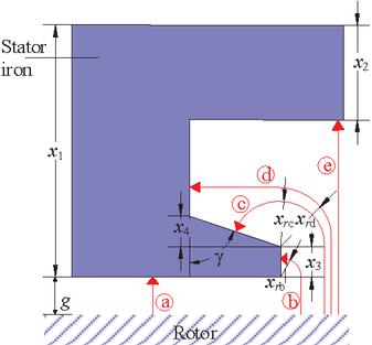
Figure 4 Ideal paths in one half of slot and tooth.

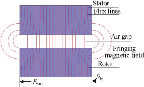
Figure 5 Air-gap fringing magnetic field for SIAFMs.

where

$\mathit{Int}(t)$	$=\sin \{{\omega }_n{R}_j[-{\omega }_{r}t+{\alpha }_{cp}(s-1)\}$
	$\times \{{\displaystyle \frac{2}{C_s}}\sin \left({\displaystyle \frac{{\omega }_n\beta }{2}}\right)\cos \left[{\displaystyle \frac{{\omega }_n(R_j{\alpha }_{cp}-\beta )}{2}}\right]$
	$+\sin \left[{\displaystyle \frac{{\omega }_n(R_j{\alpha }_{cp}-2\beta )}{2}}\right]\},$	(81)
$\mathit{Int}$	$=\{\begin{array}{cc}q{n}_t+{\displaystyle \frac{4g}{\pi }}\ln \left(1+{\displaystyle \frac{\pi q{n}_t}{4g}}\right),\hfill & m=0\hfill \\ 2{\displaystyle \frac{\sin \left(\frac{{\omega }_{m}q{n}_t}{2}\right)}{{\omega }_m}}\hfill & m\ne 0\hfill \\ \times \cos \left[{\omega }_m\left(j-{\displaystyle \frac{n_t+1}{2}}\right)q\right]\hfill & \\ +{\mathit{Int}}_1+{\mathit{Int}}_2,\hfill & \end{array},$	(86)

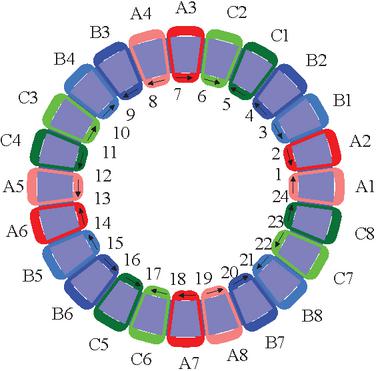
Figure 6 Coil distribution and current directions of 20-pole/24-slot SIAFMs.

Figure 6 exhibits the stator coil distribution and the current directions of a 20-pole/ 24-slot SIAFM. The instantaneous balanced three phase back-EMFs are written as

$$\{\begin{array}{c}{e}_{\mathrm{A}}=2(-e_1+e_2+e_7-e_8-e_{13}+e_{14}+e_{19}-e_{20})\hfill \\ e_{\mathrm{B}}=2(e_3-e_4-e_9+e_{10}+e_{15}-e_{16}-e_{21}+e_{22})\hfill \\ e_{\mathrm{C}}=2(-e_5+e_6+e_{11}-e_{12}-e_{17}+e_{18}+e_{23}-e_{24})\hfill \end{array},$$

(90)

where $e_{\mathrm{A}},e_{\mathrm{B}}$, and $e_{\mathrm{C}}$ are the three-phase back-EMFs, and the subscripts $1,2,\mathrm{\dots },24$ are the coil numbers.

Therefore, the electromagnetic torque for SIAFMs is

$$T_e=\frac{e_{\mathrm{A}}{i}_{\mathrm{A}}+e_{\mathrm{B}}{i}_{\mathrm{B}}+e_{\mathrm{C}}{i}_{\mathrm{C}}}{{\omega }_r},$$

(91)

where $i_{\mathrm{A}},i_{\mathrm{B}}$, and $i_{\mathrm{C}}$ are the instantaneous three-phase currents.

Table 1 Design parameters of SIAFMs

Symbol	Parameter	Value
$R_1/R_2$	Inner/outer radii of rotor iron	52/68
$r_1/r_2$	Inner/outer radii of magnets	52/68
$p/N_s$	Numbers of pole-pairs and slot	20/24
I	Rated phase current	4 A
$N$	Number of coil turns	16
${\alpha }_0$	Arc ratio of whole pole magnets	0.7
$\alpha$	Arc ratio of distance between	0.7
$g$	Air gap length	1 mm
$h$	Magnet thickness	5 mm
$B_{re}/{\mu }_r$	Magnet property	1.1
$n_e$	Rated rotational speed	3000
$P_N$	Rated power	270 W

4 OPTIMIZATION RESULTS AND FE VALIDATION

Table 1 lists the main design parameters of 20-pole/ 24-slot SIAFMs. In order to obtain the relatively better performance of the SIAFMs, optimization is made. The optimization object with the maximum average electromagnetic torque and the optimization constraint conditions are written as

$$\{\begin{array}{c}\mathrm{Max}\{\text{Average}[T_e({\alpha }_1,\mathrm{\dots },{\alpha }_{\lambda },{\theta }_1,\mathrm{\dots },{\theta }_{\lambda +1})]\}\hfill \\ \text{Subject to.}\{\begin{array}{c}0\le {\alpha }_1,\mathrm{\dots },{\alpha }_{\lambda }\le {\alpha }_0\le 1\hfill \\ 0^{\circ }\le {\theta }_1,\mathrm{\dots },{\theta }_{\lambda +1}\le {90}^{\circ }\hfill \end{array}\hfill \end{array}.$$

(109)

Based on the parameter scanning technique, Fig. 7 shows the analytically obtained average electromagnetic torque against two optimization variables (magnetization angle and pole-arc ratio) for the three-piece Halbach arrangements, and Fig. 8 shows that against three optimization variables (two magnetization angles and pole-arc ratio) for the four-piece Halbach arrangements, respectively.

Table 2 Optimized parameters for three-/four-piece Halbach

Optimized Parameters	Three-Piece	Four-Piece
${\alpha }_1$	0.29	0.39
${\theta }_1$	$/$	${17.1}^{\circ }$
${\theta }_2$	${53.0}^{\circ }$	${60.0}^{\circ }$
$T_{\max }(\mathrm{Nm})$	0.847	0.862

According to Figs. 7 and 8, for the three-/four-piece Halbach SIAFM, the optimization variables and the largest average value of electromagnetic torque are given in Table 2.

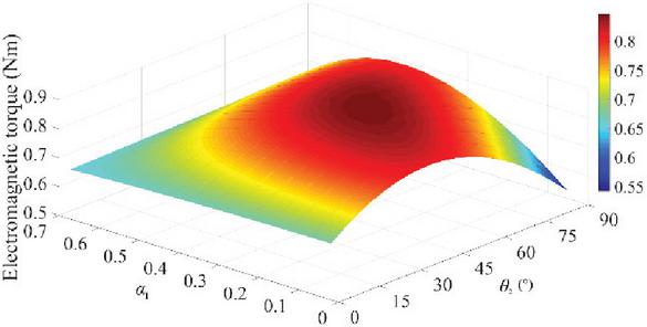
Figure 7 Analytically obtained average electromagnetic torque against pole-arc ratio and magnetization angle for three-piece Halbach.

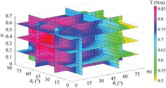
Figure 8 Analytically obtained average electromagnetic torque against pole-arc ratio and two magnetization angles for four-piece Halbach.

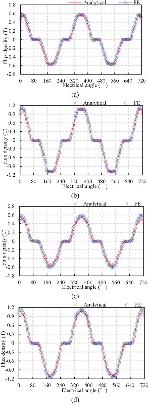
Figure 9 Flux density waveform comparison of SIAFMs with optimized three-/four-piece Halbach arrangements at different radii in the radial direction and at 5.5 mm (axial air gap center) in axial direction by 3D analytical and FE models: (a) three-piece at 26 mm, (b) three-piece at 30 mm, (c) four-piece at 26 mm, and (d) four-piece at 30 mm.

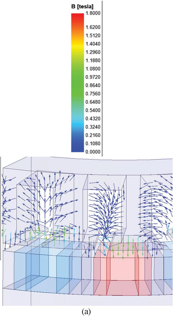
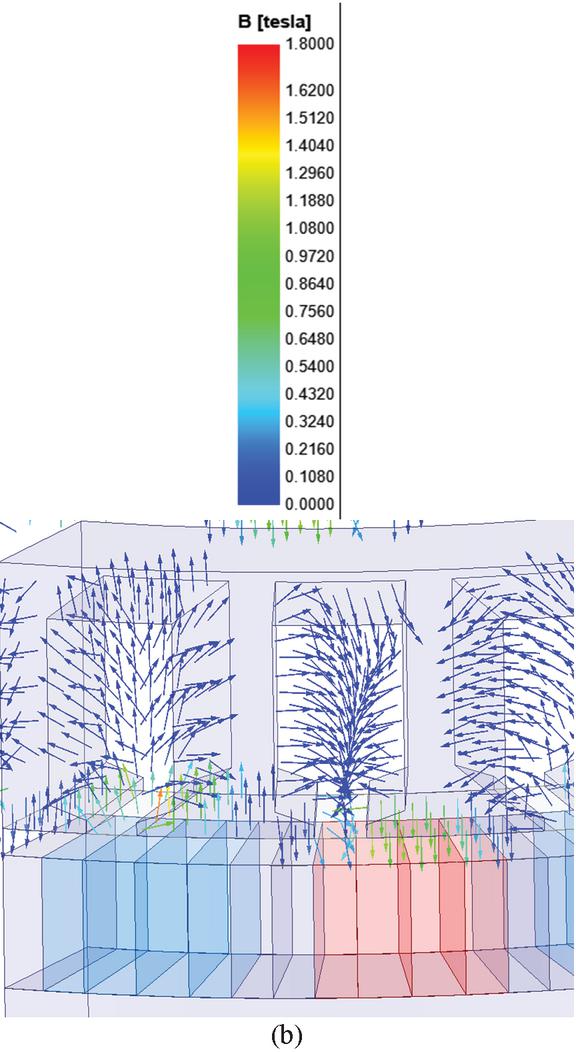
Figure 10 Magnetic flux density vector of SIAFMs with optimized three-/four-piece Halbach arrangements in 3D FE models: (a) three-piece and (b) four-piece.

Figure 9 shows a comparison of axial flux density waveforms of SIAFMs with optimized three-/four-piece Halbach arrangements at different radii by 3D FE and analytical models to verify the feasibility of the method by equivalent reluctance coefficients. It can be seen that, independent of the radius, each two waveforms calculated by two models are in great agreement.

Figure 10 shows the magnetic flux density vector of air gap and slots in SIAFMs with optimized three-/four-piece Halbach arrangements in 3D FE models. Figure 11 presents the comparison of no-load back-EMF waveforms for SIAFMs with optimized three-/four-piece Halbach arrangements from 3D FE and analytical models. It is clearly seen that great accuracy can be achieved with the use of Carter’s coefficient and the air-gap fringing field coefficient for SIAFMs.

Because the amplitude of reluctance torque for SIAFMs is lower than 1 mNm, its waveform is not given. Compared with the electromagnetic torque, its value can be ignored. Figure 12 shows that the instantaneous electromagnetic torque waveforms for 3D FE and analytical models are in good agreement for SIAFMs with both three- and four-piece Halbach arrangements. Thus, the proposed 3D analytical models are validated.

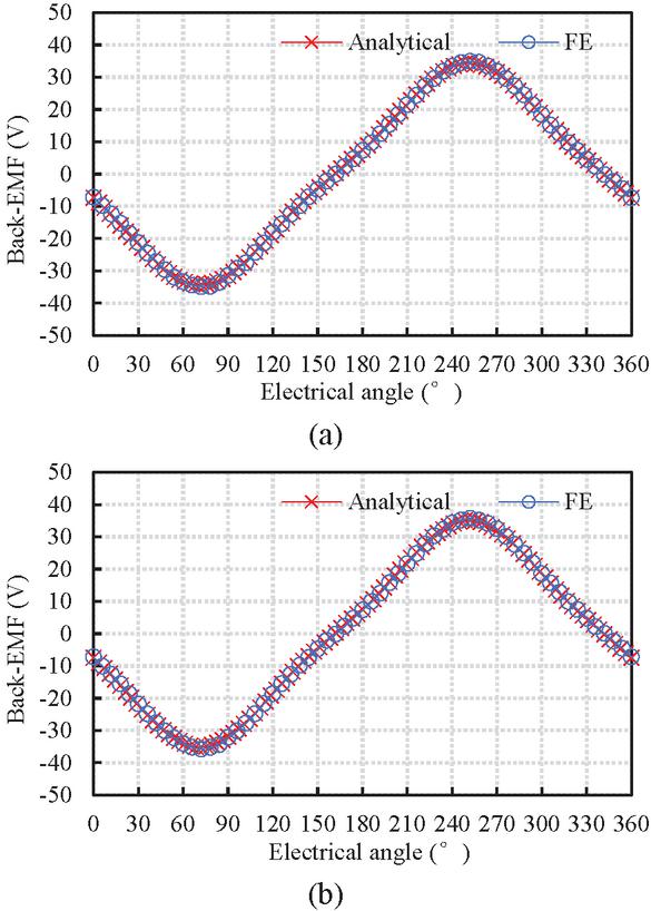
Figure 11 Comparison of back-EMF waveforms of SIAFMs with optimized three-/four-piece Halbach arrangements by 3D FE and analytical models: (a) three-piece Halbach and (b) four-piece Halbach.

Due to the presence of the radial air gap edge magnetic field, accuracy values of analytical models with/without air gap edge magnetic field are different. For SIAFMs with optimized three-/four-piece Halbach arrangements, the errors in back-EMF amplitude reduce from 9.22%/8.97% to 1.61%/1.34%, respectively. In terms of the average electromagnetic torque, the errors decrease from 7.73%/8.03% to 0.06%/0.35%, respectively.

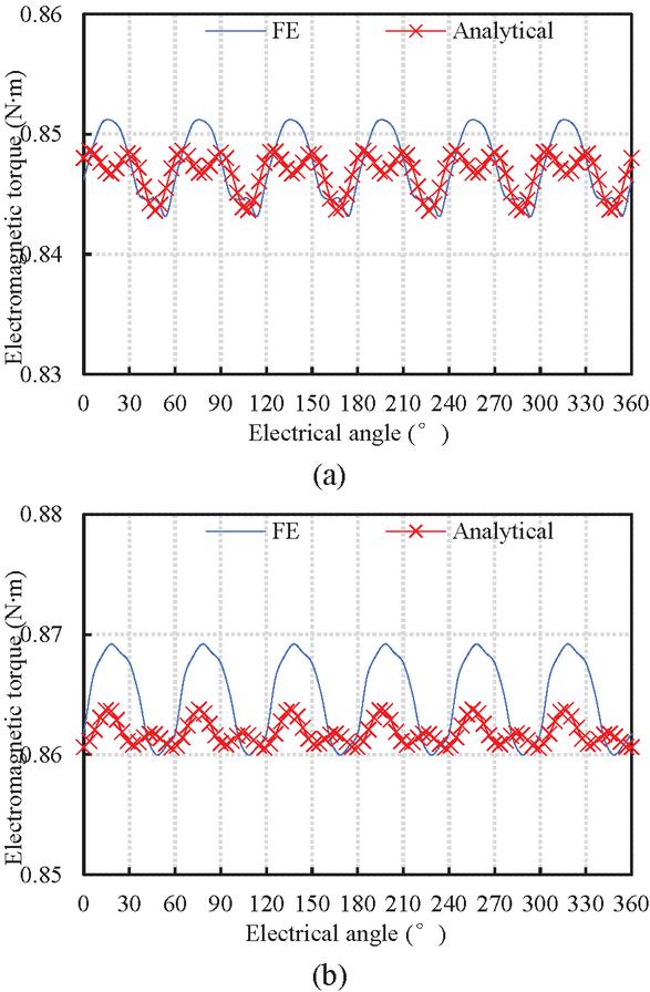
Figure 12 Comparison of electromagnetic torque waveforms of SIAFMs with optimized three-/four-piece Halbach arrangements for 3D FE and analytical models: (a) three-piece Halbach and (b) four-piece Halbach.

5 OPTIMIZATION RESULTS AND FE VALIDATION FOR SMAFMS

Similarly, Figs. 13 (a) and (b) show the PM design parameters of 2D cross section for the proposed surface-mounted odd-/even-piece Halbach arrangements, and the PM design parameters are same as those for surface-inserted odd-/even-piece Halbach arrangements. In particular, if $\alpha =1$, the SIAFMs are equivalent to the SMAFMs.

Figure 14 shows a comparison of axial flux density of slotted SMAFMs with optimized three-/four-piece Halbach arrangements by FE and 3D analytical models. It can be seen that the waveforms calculated by the two models referred to above are in great agreement.

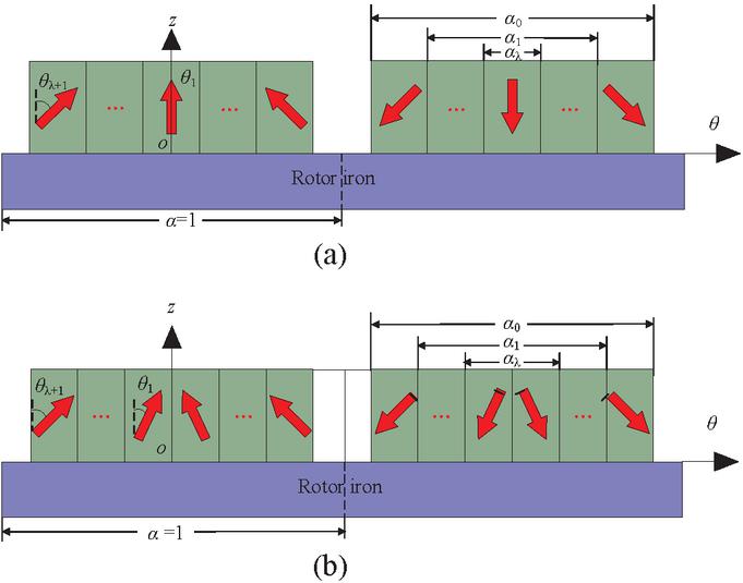
Figure 13 Design parameters of surface-mounted odd-/even-piece Halbach arrangements: (a) odd-piece Halbach and (b) even-piece Halbach.

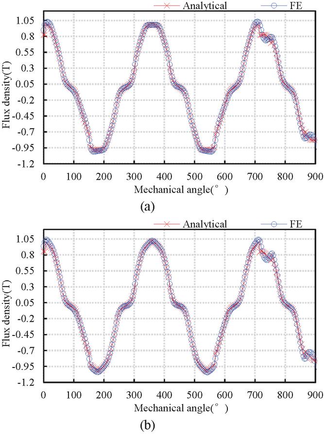
Figure 14 Flux density waveform comparison of SMAFMs with optimized three-/four-piece Halbach arrangements by FE and 3D analytical models: (a) three-piece and (b) four-piece.

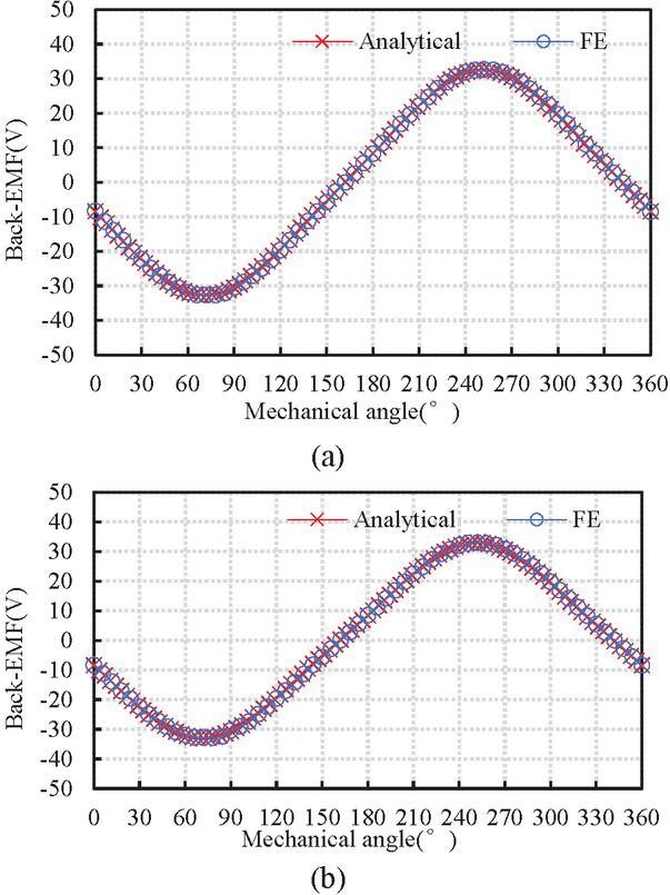
Figure 15 Comparison of back-EMF waveforms of SMAFMs with optimized three-/four-piece Halbach arrangements by FE and 3D analytical models: (a) three-piece Halbach and (b) four-piece Halbach.

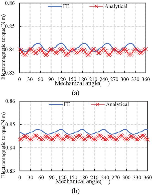
Figure 16 Comparison of electromagnetic torque waveforms of SMAFMs with optimized three-/four-piece Halbach arrangements by FE and 3D analytical models: (a) three-piece Halbach and (b) Four-piece Halbach.

Figure 15 presents a comparison of no-load backEMF waveforms of slotted SMAFMs with optimized three-/four-piece Halbach arrangements from FE and 3D analytical models. It can be clearly seen that the use of Carter’s coefficient and the air-gap outside leakage magnetic field coefficient for slotted SMAFMs exhibit great computation accuracy.

Figure 16 shows that instantaneous electromagnetic torque waveforms from FE and 3D analytical models are in excellent agreement for SMAFMs with both three- and four-piece Halbach arrangements. Thus, the 3D analytical models proposed above are validated.

6 ANALYTICAL COMPARISON WITH NON-OPTIMIZED HALBACH SIAFMS

To analyze the effects of the optimized variables and methods mentioned in section IV, this section compares the traditional Halbach array with the optimized Halbach array in terms of back EMF, harmonics, and electromagnetic torque. Figures 17 (a) and (b) show the PM design parameters of the non-optimized three-/four-piece Halbach arrangements for SIAFMs, and the detailed parameter values are listed in Table 3.

Table 3 PM parameters for non-optimized SIAFMs with three-/four-piece Halbach arrangements

Symbol	Three-Piece	Four-Piece
		Combination 1	Combination 2
$\alpha$	0.7	0.7	0.7
${\alpha }_0$	0.7	0.7	0.7
${\alpha }_1$	$7/30$	0.35	0.35
${\theta }_1{(}^{\circ })$	0	30	45
${\theta }_2{(}^{\circ })$	45	45	60

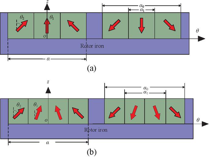
Figure 17 Design parameters of non-optimized three-/four-piece Halbach arrangements for SIAFMs: (a) three-piece Halbach and (b) four-piece Halbach.

The prediction shows that for four-piece Halbach, the performance of combination 1 is better than that of combination 2. Therefore, combination 1 is chosen for the comparison with the optimized results. Figure 18 exhibits and compares the back-EMF for the non-optimized/optimized 3D SIAFM models with three-/four-piece Halbach arrangements.

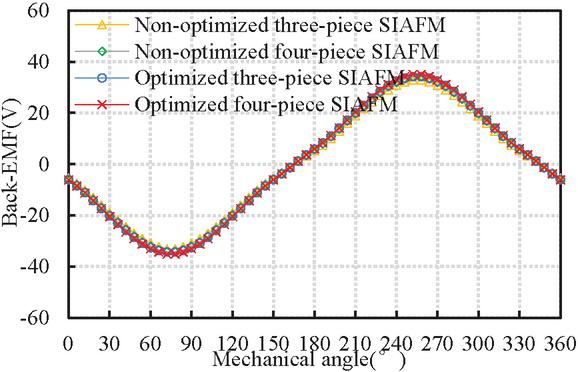
Figure 18 Comparison of back-EMF waveforms for SIAFMs with non-optimized/proposed three-/four-piece Halbach.

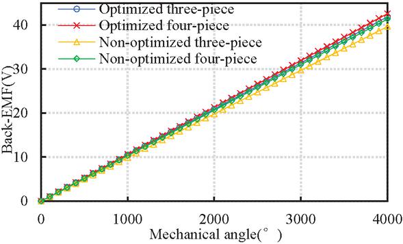
Figure 19 Comparison of fundamental component of back-EMF with respect to speed for SIAFMs with non-optimized/proposed three-/four-piece Halbach.

Figure 19 exhibits and compares the differences of fundamental component of back-EMF with respect to speed for SIAFMs with non-optimized/optimized three-/four-piece Halbach. Tables 4 and 5 list the back-EMF harmonics, total harmonic distortion (THD), and fundamental amplitude (FA) for the non-optimized/optimized SIAFMs with Halbach arrangements. It can be clearly observed that the back-EMFs of the optimized 3D SIAFM models have higher fundamental and less harmonic components than those of the non-optimized ones. Compared with the values of the electromagnetic torque, it can be seen that the amplitudes of cogging torque waveforms for both Halbach arrays are small and can be ignored.

Table 4 Back-EMF harmonics for non-optimized/ optimized three-/four-piece Halbach

Harmonic	Three-Piece		Four-Piece
Order	Non-Optimized	Optimized	Non-Optimized	Optimized
1	$100.00\%$	$100.00\%$	$100.00\%$	$100.00\%$
3	10.71%	9.49%	9.96%	9.73%
5	0.05%	0.13%	0.09%	0.12%
7	0.26%	0.04%	0.16%	0.03%
9	0.43%	0.04%	0.31%	0.31%
11	0.17%	0.35%	0.20%	0.08%
13	0.22%	0.18%	0.21%	0.17%
15	0.04%	0.04%	0.03%	0.01%
17	0.01%	0.01%	0.01%	0.01%

Table 5 Back-EMF parameters for non-optimized/ optimized three-/four-piece Halbach

	Three-Piece		Four-Piece
	Non-Optimized	Optimized	Non-Optimized	Optimized
FA (V)	29.73	31.39	31.01	31.94
THD	$10.58\%$	$9.50\%$	$9.97\%$	$9.74\%$

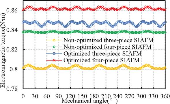
Figure 20 Comparison of torque waveforms for SIAFMs with non-optimized/optimized three-/four-piece Halbach.

Figure 20 compares the instantaneous electromagnetic torque for the 3D SIAFM models with non-optimized/optimized Halbach arrangements. As far as the electromagnetic torque values are concerned, the optimized model parameters are much better.

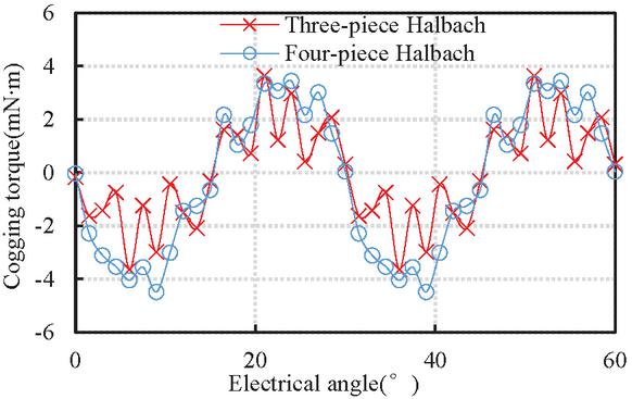
Figure 21 Cogging torque for SIAFMs with three-/four-piece Halbach.

Figure 21 shows the cogging torque for the 3D SIAFM models with proposed three-/four-piece Halbach. Figure 22 exhibits the efficiency of the machine over whole speed and torque range for the 3D SIAFM models. When the 3D SIAFM models are in constant power operation, the current and speed are inversely proportional. Therefore, as can be seen from the Fig. 22, the efficiency increases with the increase of speed.

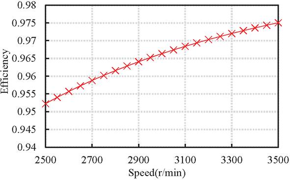
Figure 22 Efficiency of SIAFMs over whole speed and torque range.

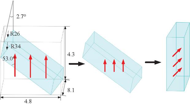
Figure 23 Manufacturing process of one Halbach magnet.

7 DISCUSSION

The manufacture of a Halbach magnet with specific magnetization angle is difficult and time-consuming and expensive. Taking one Halbach magnet segment with a specific magnetization angle as an example, the manufacturing process is shown in Fig. 23. First, a relatively large rectangular prism with parallel magnetization is manufactured. Second, the required portion of magnet is exactly cut out. Third, this magnet segment with a specific magnetization direction is placed at the desired position. Finally, all the magnet segments of Halbach array are assembled using a kind of superglue. For magnet bonding, it is essential to choose a suitable adhesive, depending on the magnet material, service environment, and strength requirements. Epoxy resin adhesive is one of the commonly used options, offering high strength, heat resistance, and chemical resistance. However, it requires mixing of two components (A and B) and has a relatively long curing time (typically 24 hours). It is often used for permanent bonding of neodymium (rare-earth) magnets and ferrite magnets to metals or plastics.

A considerable part of each magnet segment is redundant and wasteful. It can be also seen that the manufacturing process is complex and expensive. Although Halbach arrays possess excellent electromagnetic performance, their practical implementation is restricted by complicated and costly manufacturing techniques. This work focuses on applying the 3D analytical model to axial flux PM machines, using a rectangular coordinate system for derivation to avoid the complicated calculations with Bessel functions in cylindrical coordinates. It also unifies surface-mounted and surface-inserted structures into one model to evaluate the application value of Halbach arrays in axial flux PM machines. Since our research focuses on analytical modeling and design analysis rather than experimental prototyping, no physical prototype is developed in this work.

8 CONCLUSION

Different from 2D radial flux machines, the air-gap fringing effect for SIAFMs needs to be considered. Accounting for the air-gap fringing field, unified 3D analytical models are proposed for SIAFMs with odd-/even-piece Halbach arrangements. In order to obtain the correct analytical solution with high accuracy, the slotting effect is taken into account by Carter’s coefficient. Based on the proposed 3D analytical models, the constructed equations according to the interface conditions between different regions are solved and the optimized electromagnetic performances of SIAFMs with Halbach arrangements are obtained. The comparison of 3D analytical and FE predictions shows good agreement. The proposed 3D analytical models can be applied for design and optimization of SIAFMs with any-piece Halbach arrangements.

REFERENCES

[1] A. Echle, A. Neubauer, and N. Parspour, “Design and comparison of radial flux and axial flux brushless DC motors for power tool applications,” in 2018 XIII International Conference on Electrical Machines (ICEM), Alexandroupoli, Greece, pp. 125–130, 2018.

[2] A. S. Patil and R. T. Ugale, “Design and comparative analysis of axial flux and radial flux permanent magnet brushless DC motor for a 2-wheeler electric vehicle application,” in 2022 IEEE Conference on Interdisciplinary Approaches in Technology and Management for Social Innovation (IATMSI), Gwalior, India, pp. 1–4, 2022.

[3] S. Kumar, W. Zhao, Z. S. Du, T. A. Lipo, and B.-I. Kwon, “Design of ultrahigh speed axial-flux permanent magnet machine with sinusoidal back EMF for energy storage application,” IEEE Trans. Magn., vol. 51, no. 11, pp. 1–4, Nov. 2015.

[4] J. Zhu, G. Li, D. Cao, Z. Zhang, and S. Li, “Comparative analysis of coreless axial flux permanent magnet synchronous generator for wind power generation,” J. Electr. Eng., vol. 15, no. 2, pp. 727–735, 2020.

[5] B. Guo, Z. Djelloul-Khedda, and F. Dubas, “Nonlinear analytical solution in axial flux permanent magnet machines using scalar potential,” IEEE Trans. Industr. Electron, vol. 71, no. 4, pp. 3383–3393, 2024.

[6] B. Guo, Y. Huang, F. Peng, and J. Dong, “An analytical model for axial flux permanent magnet machines with Halbach array,” Chin. Soc. Electr. Eng., vol. 39, no. 1, pp. 289–295+343, 2019.

[7] Y. Cao, L. Feng, R. Mao, and K. Li, “Analysis of analytical magnetic field and flux regulation characteristics of axial-flux permanent magnet memory machine,” IEEE Trans. Magn., vol. 58, no. 9, pp. 1–9, 2022.

[8] P. Jin, Y. Yuan, Q. Xu, S. Fang, H. Lin, and S. L. Ho, “Analysis of axial-flux Halbach permanent-magnet machine,” IEEE Trans. Magn., vol. 51, no. 11, pp. 1–4, 2015.

[9] T. Okita and H. Harada, “3D analytical model of axial-flux permanent magnet machine with segmented multipole-Halbach array,” IEEE Access, vol. 11, pp. 2078–2091, 2023.

[10] S. Wu, S. Zuo, X. Wu, F. Lin, and J. Shen, “Magnet modification to reduce pulsating torque for axial flux permanent magnet synchronous machines,” Applied Computational Electromagnetics Society (ACES) Journal, vol. 31, no. 3, pp. 294–303, 2016.

[11] L. Yang, K. Yang, S. Sun, Y. Luo, F. Xiong, and C. Luo, “Study on the influence of a combined-Halbach array for the axial flux permanent magnet electrical machine with yokeless and segmented armature,” IEEE Trans. Magn., vol. 60, no. 3, pp. 1–5, 2024.

[12] Y. Huang, B. Guo, Y. Guo, J. Zhu, A. Hemeida, and P. Sergeant, “Analytical modeling of axial flux PM machines with eccentricities,” Int. J. Appl. Electromagn. Mech., vol. 53, no. 4, pp. 757–777, 2017.

[13] F. Yi, C. Zhang, S. Qiu, L. Wu, and G. Yang, “Quasi-3D analytical method of open-circuit magnetic field for yokeless and segmented armature machine,” IEEE Trans. Magn., vol. 59, no. 12, pp. 1–10, 2023.

[14] H. Tiegna, A. Bellara, Y. Amara, and G. Barakat, “Analytical modeling of the open-circuit magnetic field in axial flux permanent-magnet machines with semi-closed slots,” IEEE Trans. Magn., vol. 48, no. 3, pp. 1212–1226, 2012.

[15] A. Bellara, Y. Amara, G. Barakat, and P. Reghem, “Analytical modelling of the magnetic field in axial flux permanent magnet machines with semi-closed slots at no load,” in XIX International Conference on Electrical Machines (ICEM), Rome, Italy, pp. 1–6, 2010.

[16] W. Xu, Y. Hu, Y. Zhang, and J. Wang, “Design of an integrated magnetorheological fluid brake axial flux permanent magnet machine,” IEEE Trans. Transp. Electrif., vol. 10, no. 1, pp. 1876–1886, 2024.

[17] M. Sun, R. Tan, X. Han, and W. Tong, “Analysis and modeling for open circuit air gap magnetic field prediction in axial flux permanent magnet machines,” Chin. Soc. Electr. Eng., vol. 38, no. 5, pp. 1525–1533, 2018.

[18] F. Zhao, Z. Shao, and H. Fan, “Analytical calculation and low-order component optimization of axial electromagnetic force for an axial flux motor,” IEEE Trans. Magn., vol. 59, no. 11, pp. 1–5, 2023.

[19] J. H. Kim, Y. S. Kwon, S. Lee, B. M. Kang, J. M. Park, J. M. Sung, and J. Y. Yoon, “3D hybrid segmented layer modeling of on-load magnetic fields and torques for coreless axial-flux permanent magnet synchronous motor,” IEEE Trans. Energy Convers., vol. 38, no. 3, pp. 1815–1826, 2023.

[20] Y. Huang, B. Ge, J. Dong, H. Lin, J. Zhu, and Y. Guo, “3D analytical modeling of no-load magnetic field of ironless axial flux permanent magnet machine,” IEEE Trans. Magn., vol. 48, no. 11, pp. 2929–2932, 2012.

[21] P. Jin, Y. Yuan, M. Jin, S. Fang, H. Lin, H. Yang, and S. L. Ho, “3D analytical magnetic field analysis of axial flux permanent-magnet machine,” IEEE Trans. Magn., vol. 50, no. 11, pp. 1–4, 2014.

[22] A. Zerioul, L. Hadjout, Y. Ouazir, H. Bensaidane, A. Benbekai, and O. Chaouch, “3D analytical model to compute the electromagnetic torque of axial flux magnetic coupler with a rectangular-shaped magnet,” in 2018 International Conference on Electrical Sciences and Technologies in Maghreb (CISTEM), Algiers, Algeria, pp. 1–4, 2018.

[23] B. Dolisy, S. Mezani, T. Lubin, and J. Lévêque, “A new analytical torque formula for axial field permanent magnets coupling,” IEEE Trans. Energy Convers., vol. 30, no. 3, pp. 892–899, 2015.

[24] B. Dolisy, T. Lubin, S. Mezani, and J. Lévêque, “Three-dimensional analytical model for an axial-field magnetic coupling,” Prog. Electromagn. Res., vol. 35, pp. 173–182, 2014.

[25] A. Hemeida and P. Sergeant, “Analytical modeling of surface PMSM using a combined solution of Maxwell’s equations and magnetic equivalent circuit,” IEEE Trans. Magn., vol. 50, no. 12, pp. 1–13, 2014.

[26] Z. Q. Zhu, D. Howe, and Z. P. Xia, “Prediction of open-circuit airgap field distribution in brushless machines having an inset permanent magnet rotor topology,” IEEE Trans. Magn., vol. 30, no. 1, pp. 98–107, 1994.

BIOGRAPHIES

Youyuan Ni received the B.Eng. and Ph.D. degrees in electrical engineering from the Hefei University of Technology, Hefei, China, in 1999 and 2006, respectively. Since 2006, he has been with Hefei University of Technology, where he is currently an associate professor. His current research interest includes design and control of electric machines.

Jinsong Zou received the B.Eng. degree in electrical engineering and automation from Jiangsu University, Zhenjiang, China, in 2022. He is currently working toward the M.E. degree in electrical engineering with Hefei University of Technology. His current research interests include design of permanent magnet machines.

Yong Lin received the B.Eng. and M.S. degrees from Hefei University Technology of China in 1995 and 2002, respectively, both in automation engineering. He is currently an associate researcher. His research interests include automotive control systems and system modeling and simulation.

Anbang Wang received the B.Eng. and Ph.D. degrees from Hefei University of Technology, Hefei, China, in 2002 and 2016, respectively. Since 2016, he has been with Yangzhou Haitong Electronic Technology Co. Ltd., where he currently serves as an engineer. His research interests include power electronics and electric machine control.

ACES JOURNAL, Vol. 41, No. 6, 551–565
DOI: 10.13052/2026.ACES.J.410606
© 2026 River Publishers