Localized Plane Wave Approximation for Bodies of Revolution in Vegetation Scattering

Edward C. Michaelchuck Jr.^{1, 3}, Roger H. Lang¹, William O. Coburn², and Samuel G. Lambrakos⁴

¹Department of Electrical and Computer Engineering The George Washington University Washington, D.C. 20052, USA
EMichaelchuckJr@gwu.edu, Lang@gwu.edu

²Retired Electronics Engineer Army Research Laboratory, Adelphi, M.D. 20378, USA
KeefeCoburn@comcast.net

³Signature Technology Office

⁴Space Systems Development Division U.S. Naval Research Laboratory Washington, D.C. 20375, USA
Edward.C.Michaelchuck.civ@us.navy.mil
Samuel.G.Lambrakos.civ@us.navy.mil

Submitted On: March 12, 2026
Accepted On: May 17, 2026

ABSTRACT

Large computational electromagnetic problems for scattering from forest canopies in L-band (1–2 GHz) typically require modeling trees by a collection of lossy, dielectric cylinders and disks using Multiple Body of Revolution (MBOR) scattering techniques. MBOR techniques are desired for their computational efficiency compared to the 3-D Method of Moments (MoM). Within the vegetation environment associated with forest canopy, BORs are weakly coupled and, thus, approximations may be made to improve computational efficiency of MBOR scattering. This paper develops an efficient method to calculate the scattered fields from a lossy, finite length, dielectric cylinder, illuminated by a small current source. A small current source is representative of those on an adjacent BOR in MBOR scatter. Computational solutions to this problem exist, but those solutions are complicated and computationally expensive. Using the proposed method, a BOR is discretized into a series of discs such that far field conditions are a function of BOR radius rather than BOR length. These field conditions define the Localized Plane Wave Approximation (LPWA), which provides foundation for a more system specific MBOR scattering methodology, where BORs are harmonically independent of each other. For LPWA validation, the LPWA is compared to both analytical and computational solutions. The approximation shows good agreement within the constraints of the underlying assumptions. Finally, the method improves computational efficiency by more than an order of magnitude.

Keywords: Electromagnetic propagation in absorbing media, Method of Moments, microwave propagation, multiple body of revolution, remote sensing, scattering..

1 INTRODUCTION

Understanding microwave propagation through vegetation and forest environments is an important research topic with regards to remote sensing applications, communications, and target discrimination for military applications within these environments. For remote sensing applications, $\mathrm{P}/\mathrm{L}$-band frequencies are frequently used due to their forest canopy penetration and ionosphere penetration [1, 2, 3]. With respect to communications, the frequency bands can vary from HF to Ka-band.

Within these bands, there are various frequency regimes of interest for vegetative Radio Frequency (RF) scattering where different scattering models are employed. Depending on the application and frequency band of interest, these models generally are of two classes: radiative transfer methods [3, 4] or Distorted Born Theory (DBA) [3, 5]. For transport theory, one uses the scatterer properties to construct an extinction and phase matrix which are used in the transport equation. In transport theory, scattered powers are added incoherently, and scatterers are assumed to be in the far field of each other. For DBA theory, the scatterer properties are used in conjunction with the Foldy-Lax approximation [3, 6, 7, 8] to find the mean field in the scattering medium [9]. From this mean field, an effective medium is derived. The scatterers are then embedded in the effective medium, and the scattered fields are computed and summed coherently. Both single and higher order scattering in the effective medium can be considered.

In particular, L-band is of interest for remote sensing applications that examine backscatter from forest environments such as the Advanced Land Observing Satellite 4 (ALOS-4) launched in July 2025 by the Japanese Space Agency (JAXA) [10] and the NASA/NISAR joint US/India L/C band Synthetic Aperture RADAR (SAR) [11] that was launched on 30 July 2025. Due to the complicated nature of forest environments in L-band and its importance to communications and remote sensing, examination of Lband has been studied extensively [12, 13].

1.1 Background

Forest environments are often modeled as dielectric, lossy, Bodies of Revolution (BOR) such as cylinders, ellipsoids, and disks [13, 14, 15]. These representations cover a wide range of vegetation including tree trunks, needles, and leaves. Classical geometries are specifically chosen due to their relative simplicity and computational efficiency. Additionally, the use of classical shapes, as a discrete representation, provides a path towards simpler representations of forest environments, which by the definition of their nature appear stochastic. Upon examination of this environment and the classical shapes, the problem is well posed to combine both effective medium modeling and Multiple Body of Revolution (MBOR) scattering.

Previously, the DBA model of a singular Caucasian Fir tree was employed by Lang and Landry [16, 17]. The DBA model [18] entails discretizing a tree into cylindrical dielectric scatterers. The tree is then enclosed in a bounding cone, and the average medium dielectric constant is calculated via Foldy-Lax Theory over a series of layers within the cone via the mean field. An example bounding dielectric cone model can be viewed in Fig. 1. The $1^{\text{st}}$ and, if desired, $2^{\text{nd}}$ order scattering is calculated and coherently summed.

For the 1998 IGARSS paper by Lang et al. [16], the simulated monostatic RADAR Cross Section (RCS) results trended with the measured data, but the simulated results under-predicted the monostatic RCS by approximately 4 dB. Due to the RCS underprediction, second order scattering effects were introduced via Fresnel Double Scattering (FDS) where the scattering cross sections were predicted by the Discrete Dipole Approximation (DDA) [19, 20]. The scattering methods within the FDS-DDA model, however, underpredicted the Caucasian Fir tree RCS as well. Based on previous FEKO 3-D Method of Moments (MoM) simulations, the DDA has limitations when applied to our problem. This motivates an MBOR scattering approach.

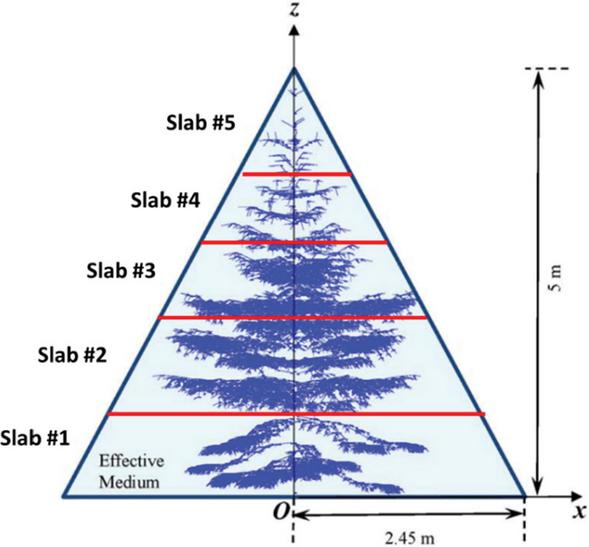
Figure 1 A 5 m Caucasian Fir tree bounded in a cone that is discretized into layers to calculate the effective medium [19].

Overall, BOR and MBOR problems have been extensively studied over the previous 70 years due to their computational efficiency compared to that of the 3D MoM [21, 22, 23, 24, 25, 26]. Recently, MBOR scattering for vegetation has been evaluated by Huang et al. where the Foldy-Lax multiple scattering equations are combined with an MBOR approach, but the model is only applied to thin cylinders where the radius is much less than a wavelength, which is representative of grass and wheat [27].

Additionally, Gu et al. has recently applied a hybrid 3D MoM approach via the combination of the T-Matrix vector cylindrical wave expansions of the scatterers and the Foldy-Lax multiple scattering equation to calculate the total scattered field of multiple trees in close proximity to one another [28]. Due to the dense vegetation environment found in the 5 m Caucasian Fir tree of interest [16, 17], the T-Matrix approach is not ideal, i.e., the cylindrical or spheroidal surfaces of the large aspect ratio cylinders would produce significant overlap regions throughout the tree model. Additionally, the T-Matrix solution does not neatly map within the existing FL/DBA model due to both the effective medium surrounding the scatterers and the multiple rays propagating within the multi-layer medium.

The method for calculating BOR scattered fields, described here, addresses certain computational problems, not well posed for solutions using T-Matrix based methods. First, unlike T-Matrix methods, the addition of spheroidal surfaces, bounding the BOR, are not required for scatterer representation. This reduction in method complexity results by imposing the volumetric condition of non-overlapping BORs, a reasonable approximation for vegetation scattering in the far-field.

Second, the method is structured formally for modeling scattered fields using effective-medium propagation constants. This formal aspect of the methodology, which should be noted for its general application, is not within the scope of this study.

In section IV, constraints are imposed for computational stability of the method, which concerns a range of cylinder aspect ratios, cylinder size to wavelength ratios, and source locations.

1.2 Objective

Our overarching objective – not the topic of this paper but described here to provide clarity to the reader – is to find the scattering amplitude of two lossy dielectric cylinders that are arbitrarily oriented with respect to each other. Each cylinder has a radius that is small compared to its length; the cylinder radius size can vary up to several wavelengths. The cylinders can be in the near field of each other but are not tightly interacting, i.e., only the first and second order scatter terms are important. The first order scattering amplitude is the bistatic scatter from each individual scatterer. The first term of the second order scattering amplitude is the scatter from the first cylinder onto the second cylinder and vice versa. The computation of the second order scatter consists of two parts: first compute the electric and magnetic surface currents on the first cylinder and, then, decompose the surface currents into dipoles. Finally, find the scattered field from the second cylinder in the presence of a dipole.

The focus of this paper is to develop a computationally efficient method to calculate the scattered fields from a lossy, finite length, dielectric BOR, e.g., a cylinder, that is illuminated by a small current source, i.e., a Hertzian dipole, in support of the goal described above. This modification expands the applicable parameter space compared to the classical thin cylinder approximation. Additionally, the technique avoids using spherical harmonics, the Mautz and Harrington approach [29, 30], by treating the incident field due to the infinitesimal current source as a local plane wave upon each BOR segment. Thus, the method is described as a Localized Plane Wave Approximation (LPWA) for arbitrary wave incidence on BORs. Although studied here in the context of vegetation scattering, the technique may be applied to any MBOR scattering problem where the BORs are not strongly coupled.

This paper will first develop a derivation for the approximation on a BOR, which also serves as a relatively direct computational encoding for this MoM implementation. An example using an electric Hertzian dipole is derived. Next, the paper validates the results of the LPWA for BORs against the full Fourier series solution, the 3-D MoM in FEKO, and an analytical solution for thin cylinders.

2 BODY OF REVOLUTION METHOD OF MOMENTS

To evaluate the scattered fields from a BOR, the Body of Revolution Method of Moments (BOR-MoM) is first developed to solve for the induced electric and fictitious magnetic surface currents due to an incident field. This derivation was developed by Mautz and Harrington [31]. The software implementation of the BOR-MoM used in this analysis was developed and validated by de Matthaeis and Lang [32, 33].

As described in [34], we restate here, for completeness, the formal mathematical foundation of our development, which is as follows. A BOR is the rotation of a generating curve, planar arc $C$, about an axis, as shown in Fig. 2. In this study, the axis of rotation will be the $z$-axis of a Cartesian coordinate system, and the generating curve will only exist in the $xz$-plane whereby the definition, the curve, $C$, is rotated ${360}^{\circ }$ around the $z$-axis. In turn, the surface, $S$, formed by the BOR, will be the interface separating free space and the scatterer with permittivity and permeability of $ϵ={ϵ}_{\mathrm{r}}{ϵ}_0$ and $\mu ={\mu }_r{\mu }_0$, respectively.

The coordinate unit vectors are defined in Fig. 2 by

$$\widehat{\mathit{\tau }}=\sin \psi \cos \phi \widehat{\mathbf{x}}+\sin \psi \sin \phi \widehat{\mathbf{y}}+\cos \psi \widehat{\mathbf{z}},$$	(1)
$$\widehat{\mathbf{n}}=\cos \psi \cos \phi \widehat{\mathbf{x}}+\cos \psi \sin \phi \widehat{\mathbf{y}}-\sin \psi \widehat{\mathbf{z}},$$	(2)
$$\widehat{\phi }=-\sin \phi \widehat{\mathbf{x}}+\cos \phi \widehat{\mathbf{y}},$$	(3)

where $\widehat{\mathit{\tau }}$ is the unit vector tangential to the generating arc, $\widehat{\mathbf{n}}$ is the unit vector normal to the generating arc, $\widehat{\mathit{\phi }}$ is the unit vector in the azimuthal direction, and $\psi$ is the angle between the $z$-axis and $\widehat{\mathit{\tau }}$ vector.

The tangential Electric Field Integral Equations (EFIE) used to evaluate the surface currents along the surface, $S$, are defined by

${\displaystyle \frac{{\mathit{E}}_{\mathrm{t}}(\mathbf{r})}{2}}$	$={\mathit{E}}_{\mathrm{t}}^{\mathrm{i}}(\mathbf{r})$
	$-\mathrm{j}\omega {\mu }_0(\underset{¯}{\mathbf{I}}-\widehat{\mathbf{n}}\widehat{\mathbf{n}})\cdot \mathrm{PV}{\displaystyle {\int }_{{\mathrm{S}}^{+}}}{\underset{¯}{\mathbf{G}}}^{(0)}(\mathbf{r},{\mathbf{r}}^{\prime })\cdot {\mathrm{J}}_{\mathrm{S}}({\mathbf{r}}^{\prime }){\mathrm{dS}}^{\prime }$
	$-(\underset{¯}{\mathbf{I}}-\widehat{\mathbf{n}}\widehat{\mathbf{n}})\cdot \mathrm{PV}{\displaystyle {\int }_{{\mathrm{S}}^{+}}}{\underset{¯}{\mathbf{K}}}^{(0)}(\mathbf{r},{\mathbf{r}}^{\prime })\times {\mathbf{M}}_{\mathrm{S}}({\mathbf{r}}^{\prime }){\mathrm{dS}}^{\prime },$	(4)
${\displaystyle \frac{{\mathit{E}}_{\mathrm{t}}(\mathbf{r})}{2}}$	$=\mathrm{j}\omega \mu (\underset{¯}{\mathbf{I}}-\widehat{\mathbf{n}}\widehat{\mathbf{n}})\cdot \mathrm{PV}{\displaystyle {\int }_{{\mathrm{S}}^{-}}}\underset{¯}{\mathbf{G}}(\mathbf{r},{\mathbf{r}}^{\prime })\cdot {\mathbf{J}}_{\mathrm{S}}({\mathbf{r}}^{\prime }){\mathrm{dS}}^{\prime }$
	$-(\underset{¯}{\mathbf{I}}-\widehat{\mathbf{n}}\widehat{\mathbf{n}})\cdot \mathrm{PV}{\displaystyle {\int }_{{\mathrm{S}}^{-}}}\underset{¯}{\mathbf{K}}(\mathbf{r},{\mathbf{r}}^{\prime })\times {\mathbf{M}}_{\mathrm{S}}({\mathbf{r}}^{\prime }){\mathrm{dS}}^{\prime },$	(5)

where ${\mathbf{E}}_{\mathrm{t}}(\mathbf{r})$ is the total, tangential, electric field on the surface, ${\mathbf{E}}_{\mathrm{t}}^{\mathrm{i}}(\mathbf{r})$ is the tangential electric field due to the incident wave, $\omega$ is the angular frequency, $\underset{¯}{\mathbf{I}}$ is the unit dyadic, PV denotes a principal value of the integral, $S^{+}$ is the outer surface of $\mathrm{S},{\mathrm{S}}^{-}$ is the inner surface of S, ${\underset{¯}{\mathbf{G}}}^{(0)}(\mathbf{r},{\mathbf{r}}^{\prime })$ is the electric dyadic Green’s function in free space, $\underset{¯}{\mathbf{G}}(\mathbf{r},{\mathbf{r}}^{\prime })$ is the electric dyadic Green’s function in the medium, ${\underset{¯}{\mathbf{K}}}^{(0)}(\mathbf{r},{\mathbf{r}}^{\prime })$ is the magnetic dyadic Green’s function in free space, $\underset{¯}{\mathbf{K}}(\mathbf{r},{\mathbf{r}}^{\prime })$ is the magnetic dyadic Green’s function in the medium, ${\mathbf{J}}_{\mathrm{s}}({\mathbf{r}}^{\prime })$ are the induced electric surface currents, and ${\mathbf{M}}_{\mathrm{s}}({\mathbf{r}}^{\prime })$ are the induced, fictitious magnetic surface currents [23].

The incident fields and induced sources within the EFIE can then be split into $\mathit{\tau }$ and $\mathit{\phi }$ vector components

${\mathit{E}}_{\mathrm{t}}^{\mathrm{i}}(\mathbf{r})$	$={\mathrm{E}}_{\tau }^{\mathrm{i}}(l,\phi )\widehat{\mathit{\tau }}+{\mathrm{E}}_{\phi }^{\mathrm{i}}(l,\phi )\widehat{\mathit{\phi }},$	(6)
${\mathbf{J}}_{\mathrm{s}}(\mathbf{r})$	$={\mathrm{J}}_{\tau }(l,\phi )\widehat{\mathit{\tau }}+{\mathrm{J}}_{\phi }(l,\phi )\widehat{\mathit{\phi }},$	(7)
${\mathbf{M}}_{\mathrm{s}}(\mathbf{r})$	$={\mathrm{M}}_{\tau }(l,\phi )\widehat{\mathit{\tau }}+{\mathrm{M}}_{\phi }(l,\phi )\widehat{\mathit{\phi }},$	(8)

where $\mathbf{r}\in S$, and the location, $\mathbf{r}$, may be expanded as a function of the azimuthal angle, $\phi$, and the location along the generating arc, $l$, i.e., $\mathbf{r}=\mathbf{r}(l,\phi )$.

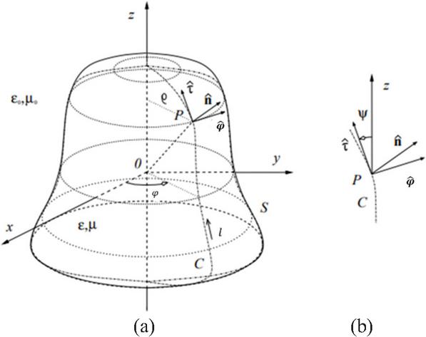
Figure 2 A body of revolution where (a) is the threedimensional model with the relevant coordinate system definitions and (b) is the coordinate definitions along the surface of the BOR.

2.1 Fourier series expansion

To evaluate the induced surface currents on the generating arc, $C$, the variables are expanded in Fourier series around the $z$-axis such that (4) and (5) needs to be only evaluated over the generating arc for a series of harmonics. The resulting incident field and induced sources are

$E_{\mathrm{t},\mathrm{p}}^{\mathrm{i}}(\mathrm{r})$	$={\displaystyle \sum _{\mathrm{n}=-\mathrm{\infty }}^{\mathrm{\infty }}}{E}_{\mathrm{t},\mathrm{p},\mathrm{n}}^{\mathrm{i}}{\mathrm{e}}^{\mathrm{jn}\phi },$	(9)
${\mathrm{J}}_{\mathrm{s},\mathrm{p}}(\mathrm{r})$	$={\displaystyle \sum _{\mathrm{n}=-\mathrm{\infty }}^{\mathrm{\infty }}}{\mathrm{J}}_{\mathrm{s},\mathrm{p},\mathrm{n}}{\mathrm{e}}^{\mathrm{j}\phi \phi },$	(10)
${\mathrm{M}}_{\mathrm{s},\mathrm{p}}(\mathrm{r})$	$={\displaystyle \sum _{\mathrm{n}=-\mathrm{\infty }}^{\mathrm{\infty }}}{\mathrm{M}}_{\mathrm{s},\mathrm{p},\mathrm{n}}{\mathrm{e}}^{\mathrm{j}\phi },$	(11)

where $\mathrm{p}\in \{\tau ,\phi \}$. The Fourier series coefficients are defined as

$$C_{p,n}=\frac{1}{2\pi }{\int }_{-\pi }^{\pi }f(\phi )e^{-jn{\phi }^{\prime }}\mathit{d}{\phi }^{\prime },$$

(12)

where ${\mathrm{C}}_{\mathrm{p},\mathrm{n}}={\mathrm{E}}_{\mathrm{t},\mathrm{p},\mathrm{n}}^{\mathrm{i}},{\mathrm{J}}_{\mathrm{s},\mathrm{p},\mathrm{n}}$, or ${\mathrm{M}}_{\mathrm{s},\mathrm{p},\mathrm{n}},\mathrm{f}(\phi )={\mathrm{E}}_{\mathrm{t},\mathrm{p}}^{\mathrm{i}},{\mathrm{J}}_{\mathrm{s},\mathrm{p}}$, or ${\mathrm{M}}_{\mathrm{s},\mathrm{p}}$, and $\mathrm{p}\in \{\tau ,\phi \}$.

2.2 Method of Moments expansion

The electric and magnetic surface currents can be discretized via the MoM such that

${\mathrm{J}}_{\mathrm{s},\tau ,\mathrm{n}}(l)$	$={\displaystyle \sum _{\mathrm{m}=1}^{\mathrm{M}}}{\mathrm{J}}_{\mathrm{s},\tau ,\mathrm{m},\mathrm{n}}(l)={\displaystyle \sum _{\mathrm{m}=1}^{\mathrm{M}}}{\displaystyle \frac{{\mathrm{\Lambda }}_{\mathrm{m},\mathrm{n}}^{\tau }{\mathrm{P}}_{\mathrm{m}}(l)}{{\rho }_{\mathrm{m}}}},$	(13)
${\mathrm{J}}_{\mathrm{s},\phi ,\mathrm{n}}(l)$	$={\displaystyle \sum _{\mathrm{m}=1}^{\mathrm{M}}}{\mathrm{J}}_{\mathrm{s},\phi ,\mathrm{m},\mathrm{n}}(l)={\displaystyle \sum _{\mathrm{m}=1}^{\mathrm{M}+1}}{\mathrm{\Lambda }}_{\mathrm{m},\mathrm{n}}^{\phi }{\mathrm{P}}_{\mathrm{m}}(l),$	(14)
${\mathrm{M}}_{\mathrm{s},\tau ,\mathrm{n}}(l)$	$={\displaystyle \sum _{\mathrm{m}=1}^{\mathrm{M}}}{\mathrm{M}}_{\mathrm{s},\tau ,\mathrm{m},\mathrm{n}}(l)={\displaystyle \sum _{\mathrm{m}=1}^{\mathrm{M}}}{\mathrm{\Omega }}_{\mathrm{m},\mathrm{n}}^{\tau }{\mathrm{P}}_{\mathrm{m}}(l),$	(15)
${\mathrm{M}}_{\mathrm{s},\phi ,\mathrm{n}}(l)$	$={\displaystyle \sum _{\mathrm{m}=1}^{\mathrm{M}}}{\mathrm{M}}_{\mathrm{s},\phi ,\mathrm{m},\mathrm{n}}(l)={\displaystyle \sum _{\mathrm{m}=1}^{\mathrm{M}+1}}{\mathrm{\Omega }}_{\mathrm{m},\mathrm{n}}^{\phi }{\mathrm{P}}_{\mathrm{m}}(l),$	(16)

where ${\mathrm{J}}_{\mathrm{s},\tau ,\mathrm{m},\mathrm{n}},{\mathrm{J}}_{\mathrm{s},\phi ,\mathrm{m},\mathrm{n}},{\mathrm{M}}_{\mathrm{s},\tau ,\mathrm{m},\mathrm{n}}$, and ${\mathrm{M}}_{\mathrm{s},\tau ,\mathrm{m},\mathrm{n}}$ are the surface currents per harmonic for their respective orthogonal and tangential vectors on each discretized segment of the generating arc, $m$ is the segment number, $M$ is the total number of segments, ${\mathrm{P}}_{\mathrm{m}}(l)$ is the chosen basis function expansion, ${\rho }_{\mathrm{m}}$ is the distance from the $z$-axis, and ${\mathrm{\Lambda }}_{\mathrm{m},\mathrm{n}}^{\tau }$, ${\mathrm{\Lambda }}_{\mathrm{m},\mathrm{n}}^{\phi }$, ${\mathrm{\Omega }}_{\mathrm{m},\mathrm{n}}^{\tau }$, and ${\mathrm{\Omega }}_{\mathrm{m},\mathrm{n}}^{\phi }$ are the basis function coefficients. Note that the basis function coefficients are unique for each harmonic, $n$, and each segment of the generating arc, $m$. For this implementation, triangular and rectangular basis functions are chosen [33].

Testing functions are now applied using the symmetric product

$$⟨\chi (l),\alpha (l)⟩={\int }_{-\mathrm{\infty }}^{\mathrm{\infty }}\chi (l)\cdot \alpha (l)dl.$$

(17)

The testing functions chosen are both Dirac Delta functions and rectangular pulse functions [31, 32, 33].

Interaction matrix and incident field matrix can be evaluated for a single harmonic on the BOR’s generating arc. The equivalent sources are solved by inverting the interaction matrix

$$[I_n]={[Z_n]}^{-1}[V_n],$$

(18)

where ${\mathrm{Z}}_{\mathrm{n}}$ is the interaction matrix. The induced surface currents per harmonic for both the $\tau$ and $\phi$ directions are described by

$${\mathrm{I}}_{\mathrm{n}}=\left[\begin{array}{c}{\mathrm{J}}_{1,\mathrm{n}}\\ {\mathrm{J}}_{2,n}\\ \mathrm{⋮}\\ {\mathrm{J}}_{N,n}\\ M_{1,\mathrm{n}}\\ M_{2,\mathrm{n}}\\ \mathrm{⋮}\\ {\mathrm{M}}_{N,n}\end{array}\right],$$

(19)

and the incident, tangential electric and magnetic fields per harmonic and for both the $\tau$ and $\phi$ directions, are described by

$${\mathrm{V}}_{\mathrm{n}}=\left[\begin{array}{c}{E}_{1,n}^i\\ E_{2,n}^i\\ \mathrm{⋮}\\ E_{M,n}^i\end{array}\right].$$

(20)

Referring to (18)–(20), the general procedure is such that ${[{\mathrm{Z}}_{\mathrm{n}}]}^{-1}$ and $[{\mathrm{V}}_{\mathrm{n}}]$ are calculated a priori, and ${\mathrm{I}}_{\mathrm{n}}$ is solved for via (18).

3 INCIDENT FIELD EXPANSION

To generate a matrix formulation for the BOR MoM, the tangential, incident electric field is expanded into Fourier series as

$${\mathit{E}}^i(\mathit{r})=\sum _{n=-\mathrm{\infty }}^{\mathrm{\infty }}{\mathit{E}}_n^i(l)e^{jn\phi },$$

(21)

where $n$ is the harmonic, $\phi$ is the azimuthal angle around the $z$-axis, and $\mathit{r}=\mathbf{r}(l,\phi )$ is the coordinate locations of the generating arc. Note that the electric field will be kept as a vector, and the subscript, $t$, will be dropped from the tangential, electric field vector. These subtle changes simplify the notation throughout this derivation. Using the definition from (12), the Fourier series coefficients are defined by

$${\mathit{E}}_n^i(l)=\frac{1}{2\pi }{\int }_{-\pi }^{\pi }{\mathit{E}}^i(l,{\phi }^{\prime })e^{-jn{\phi }^{\prime }}\mathit{d}{\phi }^{\prime },$$

(22)

where $l$ represents the location along the generating arc, the integral bounds are between $[-\pi ,\pi ]$, and $\mathit{r}=\mathit{r}(l,\phi )$. Note that the integral bounds can also be over $[0,2\pi ]$, but integrating over $[-\pi ,\pi ]$ allows for the removable singularity at zero to be integrated via the principal value of the integrals.

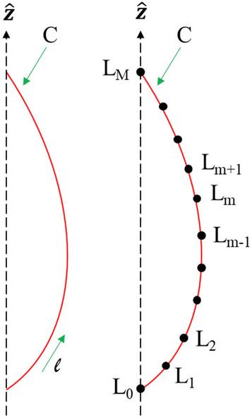
Figure 3 Discretized generating arc for a BOR.

Furthermore, the generating arc is discretized into a series of segments such that

$${\mathit{E}}^i(\mathit{r})=\sum _{m=1}^M{\mathit{E}}_m^i(l,\phi ),$$

(23)

where ${\mathit{E}}_m^i$ denotes the incident field upon a specific segment of the discretized BOR and $M$ is the total number of segments along the generating arc of the BOR, which is shown in Fig. 3. Note that ${\mathit{E}}_m^i(l,\phi )$ is unique for each segment of the BOR. Expanding ${\mathit{E}}_m^i(l,\phi )$ from (23) into a Fourier Series about the $\phi$ axis, (21) yields

$${\mathit{E}}_m^i(l,\phi )=\sum _{n=-\mathrm{\infty }}^{\mathrm{\infty }}{\mathit{E}}_{m,n}^i(l)e^{jn\phi }.$$

(24)

The total incident electric field can then be found by substituting (24) into (23) which yields

$${\mathit{E}}^i(\mathit{r})=\sum _{m=1}^M\sum _{n=-\mathrm{\infty }}^{\mathrm{\infty }}{\mathit{E}}_{m,n}^i(l)e^{jn\phi }.$$

(25)

The Fourier series coefficient in (25), ${\mathit{E}}_{m,n}^i(l)$, can be determined uniquely for each segment of the BOR generating arc by applying the Fourier Series definition from (12) to (25). Accordingly, the resultant Fourier series coefficient for a single segment and single harmonic is

$${\mathit{E}}_{m,n}^i(l)=\frac{1}{2\pi }{\int }_{-\pi }^{\pi }{\mathit{E}}_m^i(l,{\phi }^{\prime })e^{-jn{\phi }^{\prime }}\mathit{d}{\phi }^{\prime }.$$

(26)

The symmetric product of (26) with the testing functions results in the Fourier Series coefficients per harmonic in (20).

At this point in the development, an arbitrary incident field is still considered. For the exact method, derived by Harrington and Glisson [29, 30], the known, incident electric field, e.g., an incident, Hertzian dipole, is substituted into (26). The Fourier series coefficient for a single segment of the generating arc is then computed by performing the integral around the BOR $z$-axis with respect to $\phi$.

Upon examining the structure of the 5 m Caucasian Fir tree, the full expansion method is not required due to the size distribution of the branches and trunk sections. The full expansion method, however, can be applied to the MBOR scattering problem. In this case, the induced surface currents from the $1^{\text{st}}$ BOR would be treated as equivalent electric and magnetic Hertzian dipoles. Then those dipoles would be incident upon the $2^{\text{nd}}$ BOR where the full Fourier Series integration is performed. The Full Expansion method can be used to solve for the scattered fields for any size cylinder with an arbitrary distance between the cylinders, i.e., examination of trees larger than 5 m.

In general, Harrington and Mautz’s method is a relatively direct approach using spherical harmonics and reciprocity; however, the method was not designed as an MBOR scattering technique. The method requires integration around the BOR $\phi$-axis to relate the current source to the incident field upon the BOR. The introduction of multiple BORs results in harmonic dependence between the BORs and requires a large number of integrations for MBOR scattering. Thus, the full expansion method suffers a large computational burden for MBOR problem sets.

4 LOCALIZED PLANE WAVE APPROXIMATION

The following development will derive the LPWA for a vertical Hertzian dipole located on the $x$-axis and incident on a BOR. Formally, the method can be applied to an arbitrarily located and oriented dipole but, for simplicity’s sake, the dipole is oriented vertically on the $x$-axis. For application to an arbitrarily oriented dipole, the problem can be treated in a straightforward manner using local and global coordinate systems where the same approximations with respect to both the BOR radius and discretization size will still apply.

Let us consider an incident, analytical, spherical wavefront from a vertically oriented, electric, Hertzian dipole positioned along the $x$-axis, as shown in Fig. 4, whose source function is described by

$$\mathbf{J}(\mathit{r})={\mathrm{J}}_0\delta \left(\mathit{r}-{\mathit{r}}_d\right)\widehat{\mathit{z}}={\mathrm{J}}_0\delta \left(x-x_d\right)\delta (y)\delta (z)\widehat{\mathit{z}},$$

(27)

where ${\mathrm{J}}_0$ is the current density, $\delta (\mathit{r})$ is the Dirac Delta function, $\mathit{r}$ is the field location, and ${\mathit{r}}_d=x_d\widehat{\mathit{x}}$ is the source location.

To reduce the field complexity, the Hertzian dipole can be represented as a source at the origin in a local coordinate system. Following this approach, the sourcefunction simplifies to

$$\mathbf{J}(\mathit{r})={\mathrm{J}}_0\delta (\mathit{r}){\widehat{\mathbf{z}}}_d,$$

(28)

where subscript $d$ denotes that the variable is referenced to the dipole source location.

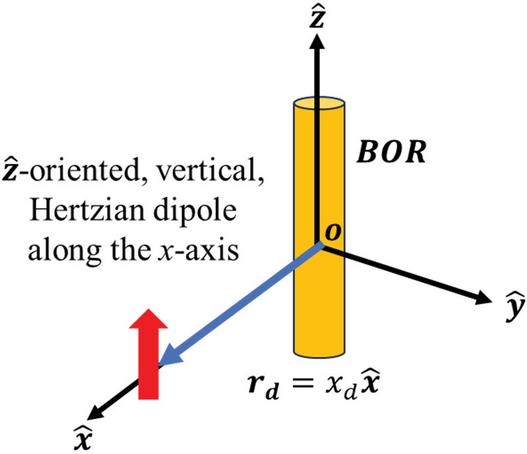
Figure 4 Vertically polarized, electric, Hertzian dipole centered on the $x$-axis incident on a BOR.

The electric field due to the source function in (28) has the general form of

$${\mathit{E}}_d^i(\mathit{r},{\mathit{r}}_d)={\mathit{E}}_{0,d}^i\frac{e^{-j{k}_0{R}_d}}{R_d},$$

(29)

where

$${\mathit{E}}_{0,d}^{\mathit{i}}=E_{r_d}^{\mathit{i}}{\widehat{\mathit{r}}}_d+E_{{\theta }_d}^{\mathit{i}}{\widehat{\mathit{\theta }}}_d,$$

(30)

and

$E_{r_d}^i$	$={\displaystyle \frac{j{\eta }_0{k}_0{J}_0}{4\pi }}\left({\displaystyle \frac{2}{j{k}_0{R}_d}}+{\displaystyle \frac{2}{{\left(j{k}_0{R}_d\right)}^2}}\right)\cos {\theta }_d,$	(31)
$E_{{\theta }_d}^i$	$={\displaystyle \frac{j{\eta }_0{k}_0{J}_0}{4\pi }}\left(1+{\displaystyle \frac{j}{j{k}_0{R}_d}}+{\displaystyle \frac{1}{{(j{k}_0{R}_d)}^2}}\right)\sin {\theta }_d,$	(32)

where ${\eta }_0$ is the free space wave impedance, $k_0$ is the free space wavenumber, ${\theta }_d$ is the polar angle in the local, spherical coordinates, and $R_d=|\mathit{r}-{\mathit{r}}_d|$.

4.1 Expansion over a BOR segment

For the following development, the spherical wave described by (28)–(32) will be adjusted such that the vectors are positional vectors with reference to a BOR segment, $m$ (see Fig. 5). This implies that the vectors can be translated from one coordinate system to another since they are referenced to an $(x,y,z)$ location. This avoids local and global coordinate transformation mathematics within the derivation.

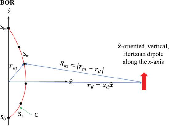
Figure 5 Diagram depicting a spherical wave source incident on a local BOR segment.

To generate the coefficients in (20) and to use the positional vectors, (29) must first be discretized across the BOR using the definition from (23). Substituting (29) into (23) yields

$${\mathit{E}}_d^i({\mathit{r}}_m,{\mathit{r}}_d)=\sum _{m=1}^M{\mathit{E}}_{0,m}^i({\mathit{r}}_m,{\mathit{r}}_d)\frac{e^{-j{k}_0{R}_m}}{R_m},$$	(33a)
$${\mathit{E}}_{0,m}^i({\mathit{r}}_m,{\mathit{r}}_d)={{\mathit{E}}_{0,d}^i|}_{r_m},$$	(33b)

where $R_m=|{\mathit{r}}_m-{\mathit{r}}_d|$.

The BOR discretized segment length can then be characterized as

$$\mathrm{\Delta }{\mathit{r}}_m={\mathit{r}}_{m+1}-{\mathit{r}}_m.$$

(34)

For small $\mathrm{\Delta }{\mathit{r}}_m,R({\mathit{r}}_m+\mathrm{\Delta }{\mathit{r}}_m,{\mathit{r}}_d)$ can be expanded as

$R({\mathit{r}}_m+\mathrm{\Delta }{\mathit{r}}_m,{\mathit{r}}_d)$
$=\sqrt{\left({\mathit{r}}_m+\mathrm{\Delta }{\mathit{r}}_m-{\mathit{r}}_d\right)\cdot \left({\mathit{r}}_m+\mathrm{\Delta }{\mathit{r}}_m-{\mathit{r}}_d\right)}$
$=\sqrt{\left({\mathit{R}}_m+\mathrm{\Delta }{\mathit{r}}_m\right)\cdot \left({\mathit{R}}_m+\mathrm{\Delta }{\mathit{r}}_m\right)}$
$=\sqrt{R_m^2+{\left(\mathrm{\Delta }{\mathit{r}}_m\right)}^2+2{\mathit{R}}_m\cdot \mathrm{\Delta }{\mathit{r}}_m}$
$=R_m\sqrt{1+{\left({\displaystyle \frac{\mathrm{\Delta }{\mathit{r}}_m}{R_m}}\right)}^2+{\displaystyle \frac{2{\mathit{R}}_m\cdot \mathrm{\Delta }{\mathit{r}}_m}{R_m^2}}}.$	(35)

Assume a small discretization and $|\frac{\mathrm{\Delta }{r}_m}{R_m}|\ll 1$. Also, note that

${[1+w]}^{1/2}$	$=1+w/2-w^2/8+O(w^3),$	(36a)
$w$	$={\left({\displaystyle \frac{\mathrm{\Delta }{\mathit{r}}_m}{R_m}}\right)}^2+{\displaystyle \frac{2{\mathit{R}}_m\cdot \mathrm{\Delta }{\mathit{r}}_m}{R_m^2}}.$	(36b)

Using the definition from (36) and assuming $|w|\ll \mathrm{\hspace{0.17em}1}$, (35) becomes

$R({\mathit{r}}_m+\mathrm{\Delta }{\mathit{r}}_m,{\mathit{r}}^{\prime })$	$=R_m\left[1+{\displaystyle \frac{\widehat{\mathit{R}}}{R_m}}\cdot \mathrm{\Delta }{\mathit{r}}_m\right]$
	$=R_m+\widehat{\mathit{R}}\cdot \mathrm{\Delta }{\mathit{r}}_m+O\left({\displaystyle \frac{\mathrm{\Delta }{\mathit{r}}_m^2}{R_m}}\right),$	(37)

where $\widehat{\mathit{R}}={\mathit{R}}_m/R_m$. The higher order terms can be neglected if the following conditions are satisfied

$$\frac{k_0{|\mathrm{\Delta }{r}_m|}^2}{2R_m}{\sin }^2\alpha \ll 1,$$

(38)

where $\alpha$ is the angle between $\widehat{\mathit{R}}$ and $\mathrm{\Delta }{\mathit{r}}_m$ and $|\frac{\mathrm{\Delta }{\mathit{r}}_m}{R_m}|\ll 1$. For $N\gg 1$, $\mathrm{\Delta }{\mathit{r}}_m$ is small and, typically, the BOR-MoM satisfies this condition using standard discretization sizes, i.e., less than or equal to a $\lambda /10$ mesh size.

Substituting (37) into (29) yields

$${\mathit{E}}_d^i({\mathit{r}}_m+\mathrm{\Delta }{\mathit{r}}_m,{\mathit{r}}_d)={\mathbf{E}}_0^{\mathrm{i}}\frac{e^{-j{k}_0(R_m+\widehat{\mathit{R}}\cdot \mathrm{\Delta }{\mathit{r}}_m)}}{R_m+\widehat{\mathit{R}}\cdot \mathrm{\Delta }{\mathit{r}}_m}.$$

(39)

Note that $R_m+\widehat{\mathit{R}}\cdot \mathrm{\Delta }{\mathit{r}}_m\approx R_m$ for small $\mathrm{\Delta }{\mathit{r}}_m$. This condition only applies to the denominator because the incident field phase, $e^{-j{k}_0(R_m+\widehat{\mathit{R}}\cdot \mathrm{\Delta }{\mathit{r}}_m)}$, has a high degree of sensitivity, whereas the incident field magnitude scaling, $\frac{1}{R_m+\widehat{\mathit{R}}\cdot \mathrm{\Delta }{\mathit{r}}_m}$, does not have a high sensitivity to error.

Expanding (39) and recognizing that $\widehat{\mathit{R}}={\widehat{\mathit{k}}}_i$ yields

$${\mathit{E}}^i({\mathit{r}}_m+\mathrm{\Delta }{\mathit{r}}_m,{\mathit{r}}_d)={\mathbf{E}}_{0,\mathrm{m}}^{\mathrm{i}}\frac{e^{-j{k}_0{R}_m}}{R_m}{e}^{-j{k}_0{\widehat{\mathit{k}}}_i\cdot \mathrm{\Delta }{\mathit{r}}_m},$$

(40)

where ${\widehat{\mathit{k}}}_i$ is the incident field unit vector. Equation (40) implies that the spherical source appears as a plane wave across the segment, i.e., the full expansion method is valid so long as (38) is valid. To solve for the coefficients in (20), substitute (40) into (26), yielding

${\mathit{E}}_{m,n}^i({\mathit{r}}_m+\mathrm{\Delta }{\mathit{r}}_m,{\mathit{r}}_d)$
$={\displaystyle \frac{1}{2\pi }}{\displaystyle {\int }_{-\pi }^{\pi }}\left[{\mathbf{E}}_{0,\mathrm{m}}^{\mathrm{i}}{\displaystyle \frac{e^{-j{k}_0{R}_m}}{R_m}}{e}^{-j{k}_0{\widehat{\mathit{k}}}_i\cdot \mathrm{\Delta }{\mathit{r}}_m}{e}^{-jn\phi }\right]\mathit{d}\phi .$	(41)

Recognize that the field coefficients of an arbitrarily sized BOR can be solved for via (41) by integrating around the BOR $\phi$-axis, so long as the BOR generating arc discretization is sufficiently small and the numerical integration converges.

4.2 Expansion around the BOR $\mathit{\phi }$-axis

At this point within the derivation, an arbitrarily sized BOR may be analyzed by integrating around the BOR $\phi$ axis, (41), for each individual segment, m. However, if thin BORs are considered, further approximations may be applied. Examining (41), it is desirable for computational efficiency to extract the spherical wave term, ${\mathbf{E}}_{0,\mathrm{m}}^{\mathrm{i}}\frac{e^{-j{k}_0{R}_m}}{R_m}$, from the integral. This would result in a localized, analytic plane wave solution over the segment, $m$.

Upon examination of the BOR cross section in Fig. 6, the BOR cross section at the local segment, $m$, is a circle by definition. The positional vector at the BOR edges can be described by

$R({\mathit{r}}_m+\mathrm{\Delta }{\mathit{\rho }}_m(\rho ,\phi ),{\mathit{r}}_d)=|{\mathit{r}}_m+\mathrm{\Delta }{\mathit{\rho }}_m(\rho ,\phi )-{\mathit{r}}_d|,$

(42)

where $\mathrm{\Delta }{\mathit{\rho }}_m(\rho ,\phi )$ is the vector between ${\mathit{r}}_m$ and the BOR edge, and $\rho$ is the radius of the BOR at segment $m$. A full expansion of $\mathrm{\Delta }{\mathit{\rho }}_m(\rho ,\phi )$ is described in [33].

Only the $\mathrm{\Delta }{\mathit{\rho }}_m(\rho ,\phi )$ term in (42) varies with respect to $\phi$. The ${\mathit{r}}_m$ term is a positional vector on the BOR generating arc, segment $m$. To extract the spherical wavefront from the integration, $\mathrm{\Delta }{\mathit{\rho }}_m(\rho ,\phi )$ must be small, therefore $\rho$ must be small.

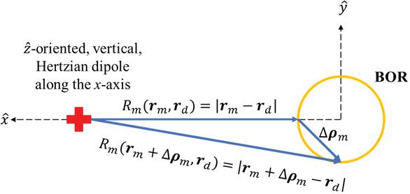
Figure 6 Spherical wave source incident on a local BOR segment.

Using this assumption, a similar development to (35)(40) can be used, i.e.,

$R({\mathit{r}}_m+\mathrm{\Delta }{\mathit{\rho }}_m,{\mathit{r}}_d)$
$=\sqrt{({\mathit{r}}_m+\mathrm{\Delta }{\mathit{\rho }}_m-{\mathit{r}}_d)\cdot ({\mathit{r}}_m+\mathrm{\Delta }{\mathit{\rho }}_m-{\mathit{r}}_d)}$
$=\sqrt{({\mathit{R}}_m+\mathrm{\Delta }{\mathit{\rho }}_m)\cdot ({\mathit{R}}_m+\mathrm{\Delta }{\mathit{\rho }}_m)}$
$=\sqrt{R_m^2+{(\mathrm{\Delta }{\mathit{\rho }}_m)}^2+2{\mathit{R}}_m\cdot \mathrm{\Delta }{\mathit{\rho }}_m}$
$=R_m\sqrt{1+{\left({\displaystyle \frac{\mathrm{\Delta }{\mathit{\rho }}_m}{R_m}}\right)}^2+{\displaystyle \frac{2{\mathit{R}}_m\cdot \mathrm{\Delta }{\mathit{\rho }}_m}{R_m^2}}},$	(43)

where $R_m=|{\mathit{r}}_m-{\mathit{r}}_d|$. Note that $r_m$ is a point along the generating arc and does not vary with respect to $\phi$. Assume a small discretization and $|\frac{\mathrm{\Delta }{\rho }_m}{R_m}|\ll 1$. Using a similar development to (36)–(38), (43) becomes

$R({\mathit{r}}_m+\mathrm{\Delta }{\mathit{\rho }}_m,{\mathit{r}}^{\prime })$	$=R_m\left[1+{\displaystyle \frac{\widehat{\mathit{R}}}{R_m}}\cdot \mathrm{\Delta }{\mathit{\rho }}_m\right]$
	$=R_m+\widehat{\mathit{R}}\cdot \mathrm{\Delta }{\mathit{\rho }}_m+O\left({\displaystyle \frac{\mathrm{\Delta }{\mathit{\rho }}_m^2}{R_m}}\right),$	(44)

with the following condition

$$\frac{k_0{|\mathrm{\Delta }{\mathit{\rho }}_m|}^2}{2R_m}{\sin }^2\beta \ll 1,$$

(45)

where $\beta$ is the angle between $\widehat{\mathit{R}}$ and $\mathrm{\Delta }{\mathit{\rho }}_m$. Substituting (44) into (41) and noting that $R_m+\widehat{\mathit{R}}\cdot \mathrm{\Delta }{\mathit{\rho }}_m\approx R_m$ for small $\mathrm{\Delta }{\mathit{\rho }}_m$ yields

${\mathit{E}}_{m,n}^i({\mathit{r}}_m+\mathrm{\Delta }{\mathit{\rho }}_m,{\mathit{r}}_d)$
$={\displaystyle \frac{1}{2\pi }}{\displaystyle {\int }_{-\pi }^{\pi }}{\mathbf{E}}_{0,\mathrm{m}}^{\mathrm{i}}{\displaystyle \frac{e^{-j{k}_0{R}_m}}{R_m}}{e}^{-j{k}_0{\widehat{\mathit{k}}}_i\cdot \mathrm{\Delta }{\mathit{\rho }}_m}{e}^{-jn\phi }\mathit{d}\phi$
$={\mathbf{E}}_{0,\mathrm{m}}^{\mathrm{i}}{\displaystyle \frac{e^{-j{k}_0{R}_m}}{R_m}}{\displaystyle \frac{1}{2\pi }}{\displaystyle {\int }_{-\pi }^{\pi }}{e}^{-j{k}_0{\widehat{\mathit{k}}}_i\cdot \mathrm{\Delta }{\mathit{\rho }}_m}{e}^{-jn\phi }\mathit{d}\phi .$	(46)

Since the ${\mathbf{E}}_{0,\mathrm{m}}^{\mathrm{i}}\frac{e^{-j{k}_0{R}_m}}{R_m}$ term no longer varies with respect to $\phi$, it was extracted from the integration, and (41) now appears as a plane wave across the BOR at segment, m. The plane wave solution for a BOR is analytical and comprised of Bessel functions [23, 33].

At this stage, the coefficients in (20) have been solved for via (46), and (46) is formally a piecewise plane wave approximation over the BOR generating arc where the initial phase and magnitude of the plane wave is the ${\mathbf{E}}_{0,\mathrm{m}}^{\mathrm{i}}\frac{e^{-j{k}_0{R}_m}}{R_m}$ term evaluated at the BOR segment ${\mathit{r}}_m$. Thus, the computational complexity of evaluating the incident field source coefficients (20) for MBOR problem set is reduced since plane wave source functions are analytical. Accordingly, (46) is termed the LPWA, allowing for analytical representation of plane waves incident on BORs.

Note that this approximation essentially turns a BOR into a set of thin discs dependent upon the free space wavenumber rather than the material wavenumber. Therefore, the far field/plane wave criteria is a function of the BOR radius rather than BOR length. In turn, the approximation error is dominated by the BOR radius since the BOR can be discretized into thinner discs, i.e., a finer mesh. Additionally, (38) and (45) establish clear criteria for monitoring a software implementation of the approximation.

4.3 Electric field coordinate expansion

The incident wave may be defined by three orthogonal unit vectors: horizontal polarization, vertical polarization, and the component of the electric field in the direction of propagation, i.e.,

${\widehat{\mathit{h}}}_i$	$={\displaystyle \frac{{\mathit{k}}_i\times \widehat{\mathit{z}}}{|{\mathit{k}}_i\times \widehat{\mathit{z}}|}}=-\sin {\phi }_i\widehat{\mathit{x}}+\cos {\phi }_i\widehat{\mathit{y}},$	(47)
$\widehat{{\mathit{v}}_i}$	$={\widehat{\mathit{h}}}_i\times {\widehat{\mathit{k}}}_i=-\cos {\theta }_i\cos {\phi }_i\widehat{\mathit{x}}-\cos {\theta }_i\sin {\phi }_i\widehat{\mathit{y}}-\sin {\theta }_i\widehat{\mathit{z}},$	(48)
${\widehat{\mathit{k}}}_i$	$=-\sin {\theta }_i\cos {\phi }_i\widehat{\mathit{x}}-\sin {\theta }_i\sin {\phi }_i\widehat{\mathit{y}}-\cos {\theta }_i\widehat{\mathit{z}},$	(49)

where ${\widehat{\mathit{h}}}_i$ is the horizontal polarization unit vector, ${\widehat{\mathit{v}}}_i$ is the vertical polarization unit vector, ${\widehat{\mathit{k}}}_i$ is the unit vector in the direction of incidence, ${\phi }_i$ is the incident, azimuthal angle, and ${\theta }_i$ is the incident, polar angle. The tangential incident field, ${\mathit{E}}_m^i$, can be described as

$${\mathit{E}}_m^i=E_{h,m}^i{\widehat{\mathit{h}}}_i+E_{v,m}^i{\widehat{\mathit{v}}}_i+E_{r,m}^i{\widehat{\mathit{k}}}_i.$$

(50)

Using the $\tau$ and $\phi$ components as defined above, (1)–(3), and combining the derived field definitions from de Matthaeis and Lang [33], the incident field becomes

$E_{\tau ,m,h}^i$	$=E_{h,m}^i\sin {\psi }_m\sin \left({\phi }_m-{\phi }_i\right)e^{-j{k}_0{\widehat{\mathit{k}}}_i\cdot {\mathit{r}}_m},$	(51)
$E_{\tau ,m,v}^i$	$=-E_{v,m}^i[\cos {\psi }_m\sin {\theta }_i$
	$+\sin {\psi }_m\cos {\theta }_i\cos ({\phi }_m-{\phi }_i)]e{}^{-j{k}_0{\widehat{\mathit{k}}}_i\cdot {\mathit{r}}_m},$	(52)
$E_{\tau ,m,r}^i$	$=-E_{r,m}^i[\cos {\theta }_i\cos {\psi }_m$
	$+\sin {\psi }_m\sin {\theta }_i\cos ({\phi }_m-{\phi }_i)]e{}^{-j{k}_0{\widehat{\mathit{k}}}_i\cdot {\mathit{r}}_m},$	(53)
$E_{\phi ,m,h}^i$	$=E_{h,m}^i\cos ({\phi }_m-{\phi }_i)e^{-j{k}_0{\widehat{\mathit{k}}}_i\cdot {\mathit{r}}_m},$	(54)
$E_{\phi ,m,v}^i$	$=E_{v,m}^i\cos {\theta }_i\sin ({\phi }_m-{\phi }_i)e^{-j{k}_0{\widehat{\mathit{k}}}_i\cdot {\mathit{r}}_m},$	(55)
$E_{\phi ,m,r}^i$	$=E_{r,m}^i\sin {\theta }_i\sin ({\phi }_m-{\phi }_i)e^{-j{k}_0{\widehat{\mathit{k}}}_i\cdot {\mathit{r}}_m}.$	(56)

The basis functions chosen in this implementation of the BOR MoM are rectangular and triangular pulses and, thus, performing the integrals for the Fourier series expansion over the basis functions yields

$E_{\tau ,m,h,n}^i$	$=j^n{E}_{h,m}^i\sin {\psi }_m{T}_n^{+}(u{\rho }_m)e^{-jn{\phi }_i}{e}^{jv{z}_m},$	(57)
$E_{\tau ,m,v,n}^i$	$=j^n{E}_{v,m}^i[-\cos {\psi }_m\sin {\theta }_i{J}_n(u{\rho }_m)$
	$++j\sin {\psi }_m\cos {\theta }_i{T}_n^{-}(u{\rho }_m)]e{}^{-jn{\phi }_i}e{}^{jv{z}_m},$	(58)
$E_{\tau ,m,r,n}^i$	$=j^n{E}_{r,m}^i[-\cos {\psi }_m\cos {\theta }_i{J}_n(u{\rho }_m)$
	$+j\sin {\psi }_m\sin {\theta }_i{T}_n^{-}(u{\rho }_m)]e{}^{-jn{\phi }_i}e{}^{jv{z}_m},$	(59)
$E_{\phi ,m,h,n}^i$	$=j^{n+1}{E}_{h,m}^i{T}_n^{-}(u{\rho }_m)e^{-jn{\phi }_i}{e}^{jv{z}_m},$	(60)
$E_{\phi ,m,v,n}^i$	$=j^n{E}_{v,m}^i\cos {\theta }_i{T}_n^{+}(u{\rho }_m)e^{-jn{\phi }_i}{e}^{jv{z}_m},$	(61)
$E_{\phi ,m,r,n}^i$	$=j^n{E}_{r,m}^i\sin {\theta }_i{T}_n^{+}\left(u{\rho }_m\right)e^{-jn{\phi }_i}{e}^{jv{z}_m},$	(62)

where ${\rho }_m$ is the radial distance from the segment $m$ to the $z$-axis. Equations (57)–(62) are the tangential fields along the generating arc of the BOR for each segment, $m$, and harmonic, $n$. The $T_n^{+}(u\rho )$ and $T_n^{-}(u\rho )$ functions are described by $J_n(x)$, the Bessel function of the first kind order $n$, i.e.,

$T_n^{+}(x)$	$={\displaystyle \frac{J_{n+1}(x)+J_{n-1}(x)}{2}},$	(63)
$T_n^{-}(x)$	$={\displaystyle \frac{J_{n+1}(x)-J_{n-1}(x)}{2}}.$	(64)

The remaining variables are described by

$$k_0{\widehat{\mathit{k}}}_i\cdot {\mathit{r}}_{\mathit{m}}=-u{\rho }_m\cos {\phi }_m-v{z}_m,$$

(65)

with

$$u=k_0\sin {\theta }_i,v=k_0\cos {\theta }_i.$$

(66)

Given that the incident electric field has been derived, derivation of the magnetic fields follows via duality, where

$H_{\tau ,m,h,n}^i$	$=j^n{H}_{h,m}^i\sin {\psi }_m{T}_n^{+}(u{\rho }_m)e^{-jn{\phi }_i}{e}^{jv{z}_m},$	(67)
$H_{\tau ,m,v,n}^i$	$=j^n{H}_{v,m}^i[-\cos {\psi }_m\sin {\theta }_i{J}_n(u{\rho }_m)$
	$+j\sin {\psi }_m\cos {\theta }_i{T}_n^{-}(u{\rho }_m)]e{}^{-jn{\phi }_i}e{}^{jv{z}_m},$	(68)
$H_{\tau ,m,r,n}^i$	$=j^n{H}_{r,m}^i[-\cos {\psi }_m\cos {\theta }_i{J}_n(u{\rho }_m)$
	$+j\sin {\psi }_m\sin {\theta }_i{T}_n^{-}(u{\rho }_m)]e{}^{-jn{\phi }_i}e{}^{jv{z}_m},$	(69)
$H_{\phi ,m,h,n}^i$	$=j^{n+1}{H}_{h,m}^i{T}_n^{-}(u{\rho }_m)e^{-jn{\phi }_i}{e}^{jv{z}_m},$	(70)
$H_{\phi ,m,v,n}^i$	$=j^n{H}_{v,m}^i\cos {\theta }_i{T}_n^{+}(u{\rho }_m)e^{-jn{\phi }_i}{e}^{jv{z}_m},$	(71)
$H_{\phi ,m,r,n}^i$	$=j^n{H}_{r,m}^i\sin {\theta }_i{T}_n^{+}(u{\rho }_m)e^{-jn{\phi }_i}{e}^{jv{z}_m}.$	(72)

Referring to (57)–(72), the field angle of incidence is unique for each segment of the BOR. The incident angle can be characterized geometrically as the angle between the incident source point, ${\mathit{r}}_d$ and $m^{\text{th}}$ segment of the BOR generating arc.

Overall, the LPWA affected a reduction of computational complexity by means of functions with lookup tables such as Bessel functions. It is interesting to note that (57)–(72) represent a rather direct computational encoding of the LPWA applied to the BOR-MoM for a Hertzian dipole source.

5 HERTZIAN DIPOLE EXAMPLE

The Hertzian dipole derivation has been implemented into a BOR MoM code to modify the incident wave upon the BOR. To validate the LPWA for a BOR, a Hertzian dipole example will be considered as a test case since it is a classical case with an exact solution, see Fig. 4. The Hertzian Dipole is vertically polarized along the $z$-axis and located at $x=0.2\mathrm{m},y=0\mathrm{m}$, and $z=0\mathrm{m}$. Thus, the dipole will be located within the reactive near field, Fresnel near field, and far field of the dielectric BOR. The BOR center is located at $x=0\mathrm{m},y=0\mathrm{m}$, and $z=$ 0 m; see Fig. 7. Note that formally the LPWA applies to magnetic surface currents as well, i.e., magnetic dipoles. For the sake of compactness, only electric dipoles are examined within this paper.

Although there are an entourage of test cases for LPWA validation, only lossy dielectric cylinders representative of a Caucasian Fir tree are examined. Additionally, the Hertzian dipole is placed along the $x$ axis to simplify the analytical solution for a thin cylinder (see Appendix A). Note that the analytical solution relies on the thin cylinder approximation where the phase across the cylinder diameter is assumed constant, i.e., the method is a function of both cylinder radius and dielectric constant [37].

The results are compared to the FEKO 3-D MoM [35] solution, the full integration method [29, 30], which entails integrating the dipole equations around the BOR $z$-axis for the full Fourier series expansion, and an analytical solution for thin cylinders. The analytical solution is in Appendix A.

5.1 Case 1: Median branch

Let us consider an incident RF field on a lossy, dielectric cylinder whose statistics are listed in Table 1, at a frequency of $f=2.0\mathrm{GHz}$. Simulation of MBOR scattering within a 5 m Caucasian Fir tree is of interest; therefore, the cylinder is the approximate size of the median branch of a Caucasian Fir tree [16, 17, 36]. The scattered far fields from the BOR due to the dipole are examined in Cartesian coordinates. The results supporting validation are shown in Figs. 8 and 9. The $x$ position and $y$-position of the scattered electric field $z$ axis sweep are at $x=10\mathrm{m}$ and $y=0\mathrm{m}$, respectively.

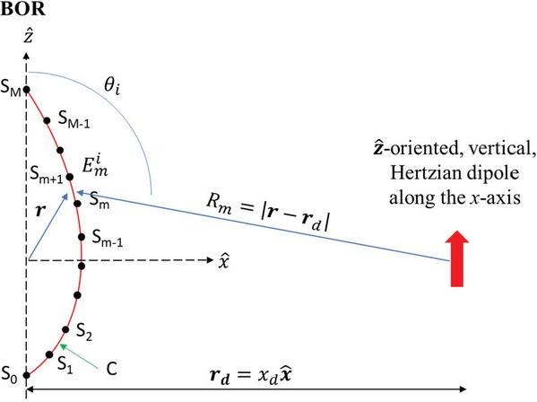
Figure 7 LPWA BOR validation scenario where a vertically polarized, Hertzian dipole is centered on the $x$-axis.

Table 1 Case 1 scenario for the LPWA with an incident Hertzian dipole for the median branch in a 5 m Caucasian Fir tree

Quantity	Value
Cylinder Length [m]	0.08
Cylinder Radius [m]	0.001
${\mathit{ϵ}}_{\mathit{r}}$	10$-$j2.4
Harmonics	10
Mesh Size	${\lambda }_{\mathrm{m}}/40$
${\mathit{r}}_{\mathit{d}}(\mathit{x},\mathit{y},\mathit{z})[\mathit{m}]$	0.2, 0, 0
Dipole Polarization	$\widehat{\mathit{z}}$ (V-Pol)
Dipole Moment [A-m]	1
$\frac{|\mathrm{\Delta }{\mathit{r}}_{\mathit{m}}|}{|{\mathit{r}}_{\mathit{m}}|}$	0.002
$\frac{\rho }{|{\mathit{r}}_{\mathit{m}}|}$	0.02

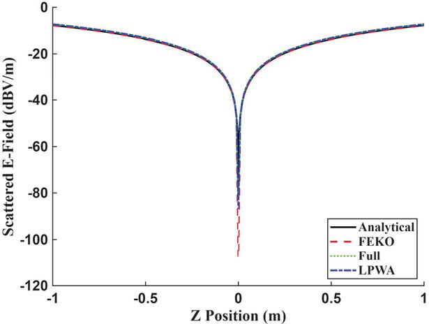
Figure 8 Median branch – $\widehat{\mathit{x}}$ polarized. Magnitude of the bistatic electric field versus $z_S$ for a V-polarized wave with $\widehat{\mathit{x}}$ polarized scattering on a dielectric cylinder at $x=$ 10 m and $y=0\mathrm{m}$. The vertically oriented dipole is located at ${\mathit{r}}_{\mathit{d}}(x,y,z)=0.2\mathrm{m},0\mathrm{m},0\mathrm{m}$.

As expected, all four methods show great agreement for a small cylinder case since the assumptions of the analytical solution and LPWA hold, i.e., $\frac{\rho }{|{\mathit{r}}_{\mathit{m}}|}$ and $\frac{|\mathrm{\Delta }{\mathit{r}}_{\mathit{m}}|}{|{\mathit{r}}_{\mathit{m}}|}$ are small.

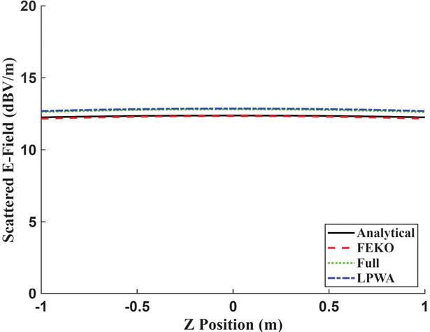
Figure 9 Median Branch – $\widehat{\mathit{z}}$ polarized. Magnitude of the bistatic electric field versus $z_S$ for a V-polarized wave with $\widehat{\mathit{z}}$ polarized scattering on a dielectric cylinder at $x=$ 10 m and $y=0\mathrm{m}$. The vertically oriented dipole is located at ${\mathit{r}}_{\mathit{d}}(x,y,z)=0.2\mathrm{m},0\mathrm{m},0\mathrm{m}$.

5.2 Cases 2 and 3: Largest branch and trunk

To ensure the LPWA method applies to the largest sections within a 5 m Caucasian Fir tree, let us consider an incident RF field on lossy, dielectric cylinders whose statistics are listed in Tables 2 and 3, at a frequency of $f=2.0\mathrm{GHz}$. The BOR size is consistent with the largest branch and largest trunk sections of a previously vectorized and measured Caucasian Fir tree [16, 17, 36]. The results supporting validation are shown in Figs. 10–13.

Table 2 Case 2 scenario for the LPWA with an incident Hertzian dipole for the largest branch in a 5 m Caucasian Fir tree

Quantity	Value
Cylinder Length [m]	0.3
Cylinder Radius [m]	0.01
${\mathit{ϵ}}_{\mathit{r}}$	$10-\mathrm{j2}.4$
Harmonics	10
Mesh Size	${\lambda }_{\mathrm{m}}/40$
${\mathit{r}}_{\mathit{d}}(\mathit{x},\mathit{y},\mathit{z})[\mathit{m}]$	$0.2,0,0$
Dipole Polarization	$\widehat{\mathit{z}}(\mathrm{V}$-Pol $)$
Dipole Moment [A-m]	1
$\frac{\left|\mathrm{\Delta }{\mathit{r}}_{\mathit{m}}\right|}{\left|{\mathit{r}}_{\mathit{m}}\right|}$	0.003
$\frac{\rho }{\left|{\mathit{r}}_{\mathit{m}}\right|}$	0.05

Table 3 Case 3 scenario for the LPWA with an incident Hertzian dipole for the largest trunk section in a 5 m Caucasian Fir tree

Quantity	Value
Cylinder Length [m]	0.5
Cylinder Radius [m]	0.05
${\mathit{ϵ}}_{\mathit{r}}$	$23-\mathrm{j5}.2$
Harmonics	10
Mesh Size	${\lambda }_{\mathrm{m}}/40$
${\mathit{r}}_{\mathit{d}}(\mathit{x},\mathit{y},\mathit{z})[\mathit{m}]$	$0.2,0,0$
Dipole Polarization	$\widehat{\mathit{z}}$ (V-Pol)
Dipole Moment [A-m]	1
$\frac{\left|\mathrm{\Delta }{\mathit{r}}_{\mathit{m}}\right|}{\left|{\mathit{r}}_{\mathit{m}}\right|}$	0.25
$\frac{\rho }{\left|{\mathit{r}}_{\mathit{m}}\right|}$	0.05

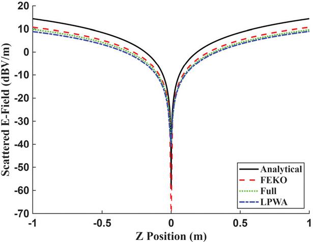
Figure 10 Largest branch – $\widehat{\mathit{x}}$ polarized. Magnitude of the bistatic electric field versus $Z_S$ for a V-polarized wave with $\widehat{\mathit{x}}$ polarized scattering on a dielectric cylinder at $x=$ 10 m and $y=0\mathrm{m}$. The vertically oriented dipole is located at ${\mathit{r}}_{\mathit{d}}(x,y,z)=0.2\mathrm{m},0\mathrm{m},0\mathrm{m}$.

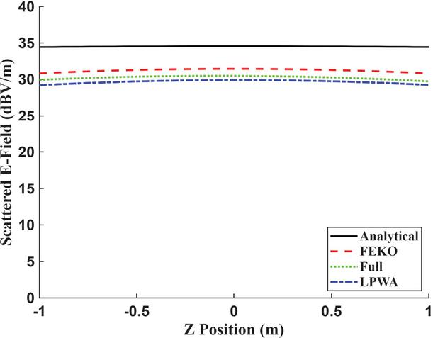
Figure 11 Largest branch – $\widehat{\mathbf{z}}$ polarized. Magnitude of the bistatic electric field versus $Z_S$ for a V-polarized wave with $\widehat{\mathit{z}}$ polarized scattering on a dielectric cylinder at $x=$ 10 m and $y=0\mathrm{m}$. The vertically oriented dipole is located at ${\mathit{r}}_{\mathit{d}}(x,y,z)=0.2\mathrm{m},0\mathrm{m},0\mathrm{m}$.

The results show a relatively small increase in error for the LPWA as the BOR radius increases. However, the solution error is still less than 0.2 dB compared to the Full Expansion solution for the branches present within the Caucasian Fir tree.

The results shown in Figs. 8–13 demonstrate computationally that the analytical, thin cylinder approximation for scattering from a dielectric cylinder is not valid when the BOR radius is large, as expected [37, 38, 39]. The analytical solution’s error increases significantly as the BOR radius increases, since the cylinders are no longer thin. This implies that the analytical solution is no longer valid when the assumptions underlying the approximations given in Appendix A are no longer satisfied. Thus, traditional thin cylinder approximation methods are not applicable for MBOR scattering of this class of Caucasian Fir tree. The LPWA, however, does not have the same BOR radius limitation as the analytical solution and, in turn, the LPWA is well suited for solving large MBOR problem sets related to tree scattering. Thus, the LPWA is an ideal method for the class of BORs expected within the 5 m Caucasian Fir tree.

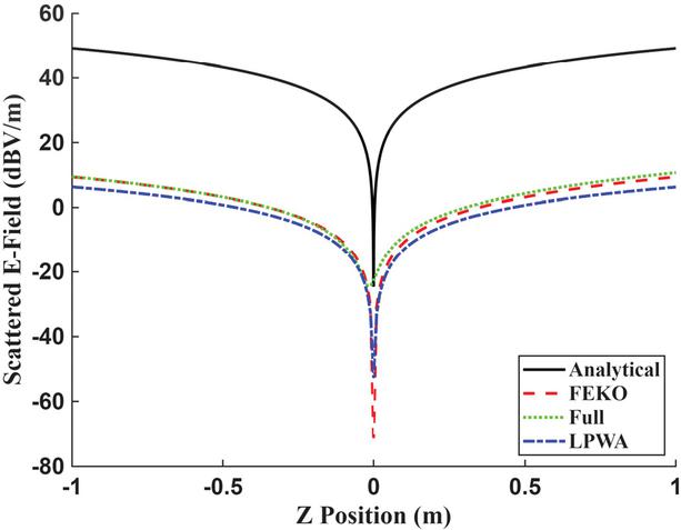
Figure 12 Largest trunk section – $\widehat{\mathit{x}}$ polarized. Magnitude of the bistatic electric field versus $z_S$ for a V-polarized wave with $\widehat{\mathit{x}}$ polarized scattering on a dielectric cylinder at $x=10\mathrm{m}$ and $y=0\mathrm{m}$. The vertically oriented dipole is located at ${\mathit{r}}_{\mathit{d}}(x,y,z)=0.2\mathrm{m},0\mathrm{m},0\mathrm{m}$.

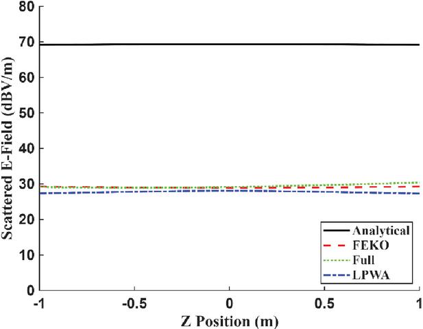
Figure 13 Largest trunk section $-\widehat{\mathit{z}}$ polarized. Magnitude of the bistatic electric field versus $Z_S$ for a V-polarized wave with $\widehat{\mathit{z}}$ polarized scattering on a dielectric cylinder at $x=10\mathrm{m}$ and $y=0\mathrm{m}$. The vertically oriented dipole is located at ${\mathit{r}}_{\mathit{d}}(x,y,z)=0.2\mathrm{m},0\mathrm{m},0\mathrm{m}$.

5.3 Error examination

The following analyses examine LPWA error tolerance. In particular, the graphs show a comparison between the full expansion method and LPWA for the electric field coefficients.

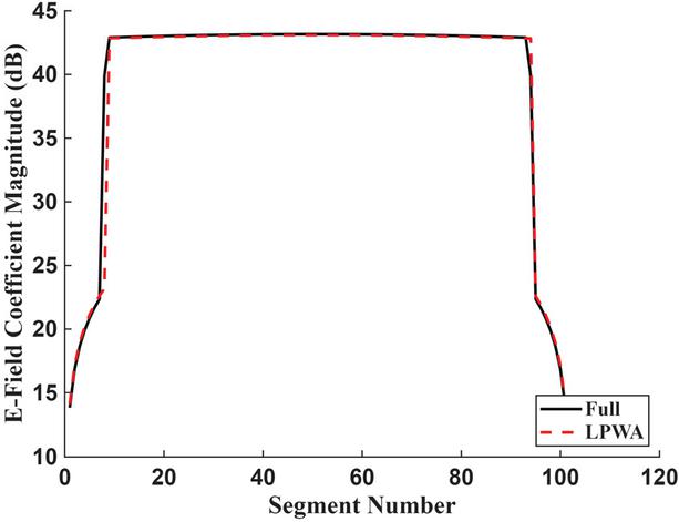
Figure 14 Incident electric field coefficient, magnitude comparison, for the $0^{\text{th}}$ harmonic, between the full expansion method and LPWA.

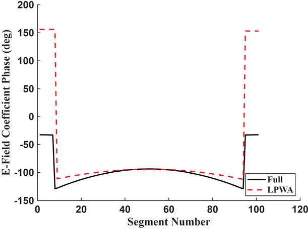
Figure 15 Incident electric field coefficient phase comparison, for the $0^{\text{th}}$ harmonic, between the full expansion method and LPWA.

A small cylinder is simulated that is 10 cm in length and 4 mm in radius like that of Case 1. The incident field is V-polarized on a dielectric cylinder at a frequency of $f=3\mathrm{GHz}$. The vertically oriented dipole is located at ${\mathit{r}}_{\mathit{d}}(x,y,z)=0.2\mathrm{m},0\mathrm{m},0\mathrm{m}$. Both magnitude and phase of the electric field coefficients at specific harmonics are plotted, shown in Figs. 14–17. Note that only the coefficients for a V-polarized wave are shown here for brevity, but both H-polarized and V-polarized coefficients have been examined.

Overall, the method shows great agreement across the cylinder body for incident electric field coefficient magnitude. The methods do differ, however, with respect to the coefficient phase. In these validation cases, the phase error primarily occurs at the corner of the cylinder and the upper cylinder segments, where the cylinder segments are perpendicular to the incident electric field.

As it relates to the transverse segment phase error, i.e., the segments on the top and bottom of the cylinder, the transverse segment current magnitudes are on the order of 20 dB lower than that of the segments parallel to the incident electric field. Thus, their induced currents and the resultant contributions to the scattered field are negligible. Additionally, the transverse segment current magnitudes have minimal error compared to the exact solution, which further supports the conclusion that transverse segment phase error is negligible relative to total scattered field error. Since the phase error has negligible impact on the total scattered fields, its source is not explored further in this paper.

To further examine the error due to BOR radius, i.e., the validity and impact of the $\frac{|\mathrm{\Delta }{\rho }_m|}{|R_m|}\ll 1$ assumption, an error plot examining the LPWA versus full expansion method with respect to BOR radius is plotted in Fig. 18. See Table 4 for simulation statistics.

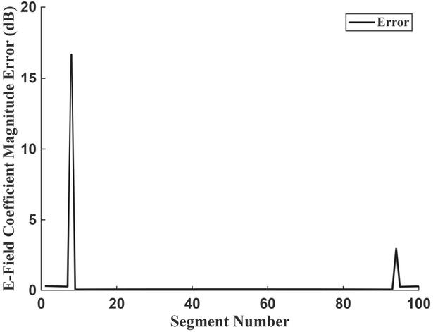
Figure 16 Incident electric field coefficient magnitude error between the full expansion method and LPWA for the $1^{\text{st}}$ harmonic.

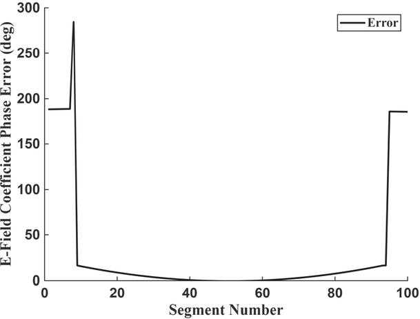
Figure 17 Incident electric field coefficient phase error between the full expansion method and LPWA for the $1^{\text{st}}$ harmonic.

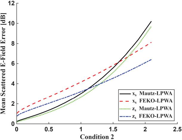
Figure 18 Far field, average, scattered electric field magnitude error between both the Mautz and LPWA methods and FEKO and LPWA methods versus Condition $2(\frac{k_0{|\mathrm{\Delta }{\rho }_m|}^2}{2R_m}{\sin }^2\beta \ll 1)$ at the scattered field point $x_s=10\mathrm{m},y_s=0\mathrm{m},z_s=0\mathrm{m}$ for a V-polarized wave incident on a dielectric cylinder.

Table 4 Error examination scenarios for the LPWA with an incident Hertzian dipole

Quantity	Value
Cylinder Length [m]	0.5
Cylinder Radius [m]	0.001, 0.01, 0.05, 0.1
${ϵ}_{\mathit{r}}$	10.3$-$j2.4
Harmonics	10
Mesh Size	${\lambda }_{\mathrm{m}}/40$
${\mathit{r}}_{\mathit{d}}\mathbf{(}\mathit{x},\mathit{y},\mathit{z})[\mathit{m}]$	0.2, 0, 0
Dipole Polarization	$\widehat{\mathit{z}}$ (V-Pol)
Dipole Moment [A-m]	1
$\frac{|\mathrm{\Delta }{\mathit{r}}_{\mathit{m}}|}{|{\mathit{r}}_{\mathit{m}}|}$	0.003, 0.003, 0.005, 0.008
$\frac{\rho }{|{\mathit{r}}_{\mathit{m}}|}$	0.005, 0.05, 0.33, 1

Figure 18 shows the average, difference error magnitude (47) between the full expansion method and LPWA for the scattered electric field in the far field. A cylinder is simulated that is 50 cm in length with various radius values. The incident field is V-polarized on a dielectric cylinder at a frequency of $f=2\mathrm{GHz}$. The vertically oriented dipole is located at ${\mathit{r}}_{\mathit{d}}(x,y,z)=0.2\mathrm{m},0\mathrm{m},0\mathrm{m}$.

As the BOR radius increases and the approximation conditions are no longer satisfied, there is an exponential increase in error (see Fig. 18), which is physically consistent and expected. In general, when the conditions specified by (38) and (45) are satisfied, i.e., $\ll$1, the LPWA error between the exact (Full expansion) method and FEKO 3-D MoM solution is less than 0.2 dB and 1 dB, respectively. With regards to the FEKO 3-D MoM solution, the additional error is not due to the LPWA, but due to error associated with a specific software implementation of this BOR-MoM and its numerical-algorithmic formulation, which typically has a magnitude difference on the order of 1 dB or less compared to the FEKO 3-D MoM. This is due to the limitations of the Mautz and Harrington BOR-MOM solution, as well as the use of low order basis functions not a topic of this paper.

When considering this error, it is important to realize that, for a multi-scatter development, the other branches will be comprised of thousands of segments orthogonal to the trunk [16, 17, 36]. Thus, a majority of the segments, i.e., point sources, will satisfy the $\frac{|\mathrm{\Delta }{\rho }_m|}{|R_m|}\ll 1$ criteria, and only a small number of segments will be susceptible to large errors – a discussion for a future paper.

5.4 Computational efficiency

With regards to computational efficiency, the BORMOM inherently is more efficient than the 3-D MoM; see reference [34] for a breakdown between this BORMoM implementation and the FEKO 3-D MoM. The efficiency of the LPWA, however, warrants further discussion.

Typically, MBOR scattering requires mapping currents to spheroidal surfaces, using T-Matrix based procedures, which is not possible for the tree scattering case considered here, as stated in section I. Other model formulations of MBOR scattering require that sources from a BOR couple to adjacent BOR, imposing the need for numerical triple integration for evaluation of the incident field matrix. Thus, a reduction of model complexity should be desirable.

Additionally, calculation of the impedance matrix is typically the slowest calculation component for the MoM. In a multi-scatter model, however, the impedance matrix is calculated once per BOR, while the incident field matrix must be calculated multiple times per BOR. For example, a tree comprised of 19,000 segments would require each BOR’s incident field matrix to be calculated 19,000 times, i.e., once per incident plane wave and once per each of the 18,999 BORs illuminating the BOR of interest. Thus, relating scattered fields from adjacent BORs would have excessive computational costs.

To validate the computational benefit of the LPWA, the LPWA incident field matrix computation time is compared to the Full Expansion integration method in Table 5 for a single harmonic. Overall, Table 5 shows that the LPWA reduces the integration cost of the method by greater than an order of magnitude per harmonic. Also, computation time for the LPWA does not scale proportionately with number of elements M, whereas the full expansion method scales linearly with number of elements.

Table 5 Comparison of the computation time of the LPWA and full expansion methods for a single harmonic

Length	M	Full Expansion Method	LPWA
$\lambda$	327	183 ms	9 ms
$3\lambda$	526	280 ms	10 ms
$6\lambda$	825	483 ms	10 ms
$10\lambda$	1223	587 ms	10 ms

Table 6 Comparison of the expected computation time of the LPWA and full expansion methods for multiple BORs with 1000 segments each evaluated over $\pm 10$ harmonics

Number of BORs	Full Expansion Method	LPWA
2	1000 s	20 s
4	6,000 s	120 s
8	28,000 s	560 s
16	120,000 s	2400 s

Notably, the LPWA is formulated to achieve a reduction in computational complexity for MBOR scenarios. Specifically, its formulation does not require integration of the field source, due to the $i^{\text{th}}$ BOR around the $j^{\text{th}}$ BOR. Table 6 shows a comparison of expected computation times, based on the results of Table 5, for an MBOR scenario, where each BOR has 1000 segments and $\pm$10 harmonics per BOR. Table 6 shows that even for a two BOR scenario, the computational cost has been reduced by more than an order of magnitude. If the $i^{\text{th}}$ BOR is treated as a singular source, rather than a collection of sources, computation time for the LPWA can be decreased even further. This follows in that the full expansion method must treat each segment as a singular source.

The test cases were run on a computer with an Intel i910900k CPU overclocked to 4.9 GHz all core, 64 GB of 3600 MHz DDR4 RAM, and a Samsung 970 Evo Plus NVMe SSD. For this analysis, the software implementation was programmed in MATLAB 2025a, and the code is parallelized and vectorized to maximize computational efficiency. If this program were deployed in C++ rather than MATLAB, it is estimated to improve the computation times by another order of magnitude.

6 CONCLUSION

This analysis resulted in the derivation and relatively direct computational encoding of an arbitrary wave incident on a BOR for the MoM using the LPWA. Both the incident, tangential, electric, and magnetic fields on both the discretized $\tau$ and $\phi$ segments of the BOR were derived.

The derived equations demonstrated two approaches to the problem including a full expansion method at each segment for arbitrary BOR size, and a LPWA for thin BORs. For the full expansion method, it is assumed that the discretization is small along the generating arc and around the BOR $\phi$-axis. When the BOR radius is not large compared to wavelength, we can further simplify the procedure resulting in a source function that is a local plane wave across the whole disk, effectively reducing the far field condition to a function of BOR radius rather than BOR length. Additionally, both of the approximations apply to thicker cylinders than the analytical solution using the thin cylinder approximations. For practical applications, the far field criterion, (38) and (45), can be monitored, and the BOR separation and/or discretization can be adjusted to shrink the parameters as needed.

The derivation was verified and validated using a Hertzian dipole example and compared to the FEKO 3D MoM [35] solution, the full expansion method [29, 30], and the analytical solution for a thin cylinder. The results showed good agreement between the different MoM implementations for scattered field magnitude. In turn, the resulting computational benefit due to the reduced integration complexity of the LPWA resulted in a minimal loss of accuracy to the solution.

Overall, the error induced by the LPWA is acceptable for the specific multi-scatter approach in development for a 5 m Caucasian Fir tree since the trunk sizes, branch sizes, and branch separations examined in this paper are typical of the vectorized Caucasian Fir tree [16, 17, 36]. Additionally, the method is well posed to manage propagation between discrete scatterers when a complex medium is present, e.g., vegetative environments. The next steps are to apply the LPWA to MBOR scattering.

ACKNOWLEDGMENT

This work is supported by the U.S. Military and funded through the U.S. Naval Research Laboratory Edison Memorial Graduate Training Program.

REFERENCES

[1] F. T. Ulaby, D. G. Long, and M. Press, Microwave Radar and Radiometric Remote Sensing. Ann Arbor, MI: The University Of Michigan Press, 2014.

[2] M. E. Davis, Foliage Penetration Radar: Detection and Characterization of Objects under Trees. Raleigh, NC: Scitech Pub, 2011.

[3] L. Tsang, J. A. Kong, and R. T. Shin, Theory of Microwave Remote Sensing. Hoboken, NJ: Wiley-Interscience, 1985.

[4] M. Salim, S. Tan, R. D. De Roo, A. Colliander, and K. Sarabandi, “Passive and active multiple scattering of forests using radiative transfer theory with an iterative approach and cyclical corrections,” IEEE Transactions on Geoscience and Remote Sensing, vol. 60, pp. 1–16, 2022.

[5] R. H. Lang and J. S. Sidhu, “Electromagnetic backscattering from a layer of vegetation: A discrete approach,” IEEE Transactions on Geoscience and Remote Sensing, vol. GE-21, no. 1, pp. 62–71, Jan. 1983.

[6] L. L. Foldy, “The multiple scattering of waves. I. General theory of isotropic scattering by randomly distributed scatterers,” Physical Review, vol. 67, no. 3-4, p. 107, 1945.

[7] M. Lax, “Multiple scattering of waves,” Rev. Modern. Phys., vol. 23, pp. 287–310, 1951.

[8] M. Lax, “Multiple scattering of waves II. The effective field in dense systems,” Phys. Rev., vol. 85, pp. 261–269, 1952.

[9] A. K. Fung, “Scattering from a vegetation layer,” IEEE Transactions on Geoscience Electronics, vol. 17, no. 1, pp. 1–6, Jan. 1979.

[10] T. Motohka, Y. Kankaku, S. Miura, and S. Suzuki, “Overview of ALOS-2 and ALOS-4 L-band SAR,” in 2021 IEEE Radar Conference (RadarConf21), Atlanta, GA, USA, pp. 1–4, 2021.

[11] P. Rosen, S. Hansley, W. N. Edelstein, Y. Kim, T. Misra, R. Bhan, S. Shaffer, R. Kumar, and S. Sagi, “The NASA-ISRO SAR (NISAR) mission dual-band radar instrument preliminary design,” in 2017 IEEE International Geoscience and Remote Sensing Symposium, Fort Worth, TX, USA, pp. 3832–3835, 2017.

[12] N. S. Chauhan, R. H. Lang, and K. J. Ranson, “Radar modeling of a boreal forest,” IEEE Transactions on Geoscience and Remote Sensing, vol. 29, no. 4, pp. 627–638, July 1991.

[13] M. A. Karam, Y. M. M. Antar, and A. K. Fung, “Radar backscattering from vegetation targets,” in 1990 Symposium on Antenna Technology and Applied Electromagnetics, Winnipeg, MB, Canada, pp. 596–601, 1990.

[14] S. H. Yueh, J. A. Kong, J. K. Jao, R. T. Shin, and T. Le Toan, “Branching model for vegetation,” IEEE Transactions on Geoscience and Remote Sensing, vol. 30, no. 2, pp. 390–402, Mar. 1992.

[15] R. H. Lang, R. Landry, O. Kavaklioglu, and J.-C. Deguise, “Simulation of microwave backscatter from a red pine stand,” in Proc. SPIE 2314, Multispectral and Microwave Sensing of Forestry, Hydrology, and Natural Resources, 31 Jan. 1995.

[16] R. H. Lang, R. Landry, A. Franchois, G. Nesti, and A. Sieber, “Microwave tree scattering experiment: Comparison of theory and experiment,” in IGARSS ’98. Sensing and Managing the Environment. 1998 IEEE International Geoscience and Remote Sensing. Symposium Proceedings, Seattle, WA, USA, vol. 5, pp. 2384–2386, 1998.

[17] R. Landry, R. A. Fournier, F. J. Ahern, and R. H. Lang, “Tree vectorization: A methodology to characterize fine tree architecture in support of remote sensing models,” Canadian Journal of Remote Sensing, vol. 23, no. 2, pp. 91–107, 1997.

[18] R. H. Lang, “Electromagnetic backscattering from a sparse distribution of lossy dielectric scatterers,” Radio Science, vol. 16, no. 1, pp. 15–30, Jan.–Feb. 1981.

[19] Q. Zhao and R. H. Lang, “Scattering from tree branches using the Fresnel Double Scattering approximation,” in 2011 IEEE International Geoscience and Remote Sensing Symposium, Vancouver, BC, Canada, pp. 1040–1043, 2011.

[20] R. J. Hooker and R. H. Lang, “A successive scattering methodology with application to two cylinders in the Fresnel region of each other,” Waves in Random and Complex Media, vol. 22, no. 2, pp. 267–304, 2012.

[21] A. W. Glisson and D. R. Wilton, “Simple and efficient numerical techniques for treating bodies of revolution,” RADC-TR-79-22, Rome Air Development Center, Air Force Systems Command, Griffiss Air Force Base, New York 13441, 16 Apr. 1979.

[22] M. Andreasen, “Scattering from bodies of revolution,” IEEE Transactions on Antennas and Propagation, vol. 13, no. 2, pp. 303–310, Mar. 1965.

[23] J. R. Mautz and R. F. Harrington, “Radiation and scattering from bodies of revolution,” Appl. Sci. Res., vol. 20, pp. 405–435, 1969.

[24] T.-K. Wu and L. L. Tsai, “Scattering from arbitrarily-shaped lossy dielectric bodies of revolution,” Radio Sci., vol. 12, no. 5, pp. 709–718, 1977.

[25] A. Kishk and L. Shafai, “Different formulations for numerical solution of single or multibodies of revolution with mixed boundary conditions,” IEEE Transactions on Antennas and Propagation, vol. 34, no. 5, pp. 666–673, May 1986.

[26] M. Jiang, Y. Li, Z. Rong, L. Lei, Y. Chen, and J. Hu, “Fast solving scattering from multiple bodies of revolution with arbitrarily metallic-dielectric combinations,” IEEE Transactions on Antennas and Propagation, vol. 67, no. 7, pp. 4748–4755, July 2019.

[27] H. Huang, L. Tsang, E. G. Njoku, A. Colliander, T.-H. Liao, and K.-H. Ding, “Propagation and scattering by a layer of randomly distributed dielectric cylinders using Monte Carlo simulations of 3D Maxwell equations with applications in microwave interactions with vegetation,” IEEE Access, vol. 5, pp. 11985–12003, 2017.

[28] W. Gu, L. Tsang, A. Colliander, and S. Yueh, “Hybrid method for full-wave simulations of forests at L-band,” IEEE Access, vol. 10, pp. 105898–105909, 2022.

[29] A. Glisson and C. Butler, “Analysis of a wire antenna in the presence of a body of revolution,” IEEE Transactions on Antennas and Propagation, vol. 28, no. 5, pp. 604–609, Sep. 1980.

[30] R. F. Harrington and J. R. Mautz, “Green’s functions for surfaces of revolution,” Radio Science, vol. 7, no. 5, pp. 603–611, May 1972.

[31] J. R. Mautz and R. F. Hanington, “H-field, E-field, and combined field solutions for conducting bodies of revolution,” Arch. Elek. Ubertragung, vol. 32, pp. 157–164, 1978.

[32] P. de Matthaeis and R. H. Lang, “Comparison of surface and volume currents models for electromagnetic scattering from finite dielectric cylinders,” IEEE Transactions on Antennas and Propagation, vol. 57, no. 7, pp. 2216–2220, July 2009.

[33] P. de Matthaeis and R. H. Lang, “Numerical calculations of microwave scattering from dielectric structures used in vegetation models,” Ph.D. dissertation, Chapter 4, pp. 60–113, The George Washington University, D.C., 2006.

[34] E. C. Michaelchuck Jr., S. G. Lambrakos, and W. O. Coburn, “Near field scatter from a body of revolution,” Applied Computational Electromagnetics Society (ACES) Journal, vol. 39, no. 05, pp. 376–389, May 2024.

[35] Altair Feko, Altair Engineering Inc., Troy, Michigan, USA.

[36] Q. Zhao and R. H. Lang, “Methodology of modeling multiple scattering effects in microwave remote sensing of vegetation,” Ph.D. thesis, The George Washington University, D.C., May 2013.

[37] D. LeVine, “The radar cross section of dielectric disks,” IEEE Transactions on Antennas and Propagation, vol. 32, no. 1, pp. 6–12, Jan. 1984.

[38] D. M, Levine, A. Schneider, R. H. Lang, and H. G. Carter, “Scattering from thin dielectric disks,” Technical Memorandum, NASA, 19850006789, Sep. 1984.

[39] R. Lang, A. Schneider, S. Seker, and F. Altman, “UHF radiowave propagation through forests,” Research and Development Technical Report, CECOM-81-0136-4, 1982.

BIOGRAPHIES

Edward C. Michaelchuck Jr. is currently pursuing a Ph.D. in electrical engineering with a focus in applied electromagnetics at The George Washington University, Washington, D.C., USA. He received an M.S. degree in electrical engineering with a concentration in applied electromagnetics from George Washington University, Washington, D.C., in January 2021. He received a B.S. in mechanical engineering from Rowan University, Glassboro, NJ, in May 2017. He has been a research engineer at the Signature Technology Office, Code 5009, at the U.S. Naval Research Laboratory, Washington, D.C., since August 2017. His expertise includes multispectral signature characterization, computational electromagnetics, material measurements ranging from RF to the visible spectrum, and metamaterial design and fabrication.

Roger H. Lang (Life Fellow, IEEE) received the B.S. (1962) and M.S. (1964) degrees in Electrical Engineering and the Ph.D. degree (1968) in Electrophysics from the Polytechnic Institute of Brooklyn, New York, NY, USA (now Tandon School of Engineering, New York University). He did his postdoctoral research in random media under Joe Keller at the Courant Institute of Mathematical Sciences, New York University, New York, NY. He is currently a Professor Emeritus of Engineering and Applied Science at George Washington University, Washington, D.C., and a Research Professor in the Department of Electrical and Computer Engineering there.

He is known for the early development of the discrete scattering model for vegetation. More recently, he has been involved in remote sensing of seawater salinity and soil moisture under vegetation. His research interests include microwave remote sensing, electromagnetic wave propagation, and dielectric measurements. Lang received the Distinguished Achievement Award from the IEEE Geoscience and Remote Sensing Society. He is an Active Participant in the IEEE Geoscience and Remote Sensing Society. He was an Associate Editor for Microwave Scattering and Propagation, and the co-chair of the Technical Program Committee for the IGARSS’90 meeting held at College Park, MD, in 1990. He was the Chair of the International URSI Commission F and is a member of the Editorial Board of Waves in Random and Complex Media.

William O. Coburn received his B.S. in Physics from Virginia Polytechnic Institute, USA, in 1984. He received an M.S.E.E. in Electro Physics in 1991 and a Ph.D. in Electromagnetic Engineering from The George Washington University in 2005. His dissertation research was on traveling wave antenna design. He has 38 years’ experience as an Electronics Engineer at the Army Research Laboratory (formerly the Harry Diamond Laboratories) primarily in CEM for EMP coupling/hardening, HPM, target signatures and antennas. He retired in 2019 from the RF Electronics Division of the Sensors and Electron Devices Directorate applying CEM tools for antenna design and EM analysis.

He is a Fellow of the Applied Computational EM Society (ACES) and served on the ACES Board of Directors. He is a Member of the USNC-URSI, Commission A and B (2010), Sigma Xi and an Adjunct Professor at the Catholic University of America and GWU. Coburn has authored or coauthored over 100 publications and four patents.

Samuel G. Lambrakos received the Ph.D. degree in Physics from the Polytechnic Institute of New York University, USA, in 1983. He is a Research Physicist at the U.S. Naval Research Laboratory, Washington, D.C., where he has been for over 40 years. His expertise is computational physics in general and has many publications, patents and awards. His recent studies concern computational materials physics and inverse spectral analysis.

APPENDIX A

The following development is an abbreviated derivation for the analytical solution of a dipole incident on a thin cylinder.

Following a similar development to section IV, let the axis shifted Hertzian dipole have the following source function in a local coordinate system, see Fig. A.1,

$$\mathit{J}({\mathit{r}}_d)=J_0\delta (\mathit{r}-{\mathit{r}}_d){\widehat{\mathbf{z}}}_d.$$

(A.1)

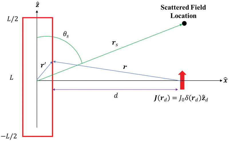
Figure A.1: Geometry of a Hertzian dipole incident on a cylinder.

Assuming $kr\gg 1$, the electric field due to the source function in (29) has the general form of

$${\mathit{E}}_d^i(\mathit{r},{\mathit{r}}_d)=E_0\sin {\theta }_d\frac{e^{-j{k}_{0}r}}{r}\widehat{\mathit{\theta }},$$	(A.2)
$$E_0=\frac{j{\eta }_0{k}_0{J}_0}{4\pi }.$$	(A.3)

Since the cylinder is thin, i.e., $a$ is small, the internal electric field may be described by

$${\mathit{E}}_{\mathit{int}}\approx {\mathit{E}}_{\parallel }+\frac{2}{1+{ϵ}_r}{\mathit{E}}_{⟂},$$

(A.4)

where ${\mathit{E}}_{\mathit{int}}$ is the internal field [37, 38, 39] and

$${\mathit{E}}_{\parallel }=E_0{\sin }^2{\theta }_d\frac{e^{-j{k}_0{R}_d}}{R_d}\widehat{\mathbf{z}},$$	(A.5)
$${\mathit{E}}_{⟂}=-E_0\sin {\theta }_d\frac{e^{-j{k}_0{R}_d}}{R_d}\cos {\theta }_d\widehat{\mathit{x}},$$	(A.6)

where ${\theta }_d$ is the angle that $\mathit{r}$ makes with the z-axis of the local coordinate system of the dipole.

Using LeVine et al. [37], the scattered electric field may be described by

$${\mathit{E}}_{\mathrm{s}}({\mathit{r}}_s)=k_0^2{\int }_V({ϵ}_r-1)\underset{¯}{\mathit{G}}(\mathit{r},{\mathit{r}}^{\prime })\cdot {\mathit{E}}_{\mathit{int}}({\mathit{r}}^{\prime })\mathit{d}{\mathit{r}}^{\prime },$$

(A.7)

where $\underset{¯}{\mathit{G}}(\mathit{r},{\mathit{r}}^{\prime })$ is the dyadic Green’s function.

Consider a scattered field location along the $z$-axis $(z_s)$ at a distance $x_s$ with $y_s=0$. To simplify the integral for the analytical solution, make the following assumptions: $ka\ll 1,\frac{z_s}{r_s}\ll 1,\frac{x_s}{r_s}\approx 1$, and $R_d^{\prime }$ is constant over the cross section of a cylinder. Substituting (A.4) into (A.7), and performing the algebraic and geometric simplifications yields

$${\mathit{E}}_{\mathrm{s}}({\mathit{r}}_s)={\mathit{E}}_{\mathrm{x}}({\theta }_s)\widehat{\mathit{x}}+{\mathit{E}}_z({\theta }_s)\widehat{\mathit{z}},$$

(A.8)

where

${\mathit{E}}_{\mathrm{x}}({\theta }_s)$	$=E_{\mathrm{d0}}[P_x^{+}{I}^{+}({\theta }_s)+P_x^{-}{I}^{-}]{\displaystyle \frac{e^{-j{k}_0{r}_s}}{r_s}},$	(A.9)
${\mathit{E}}_z({\theta }_s)$	$=E_{\mathrm{d0}}[P_z^{+}{I}^{+}+P_z^{-}{I}^{-}]{\displaystyle \frac{e^{-j{k}_0{r}_s}}{r_s}},$	(A.10)

and

$$P_x^{+}({\theta }_s)=-\frac{1}{2}\sin (2{\theta }_s),$$	(A.11)
$$P_x^{-}({\theta }_s)={\sin }^2({\theta }_s),$$	(A.12)
$$P_z^{+}({\theta }_s)={\cos }^2({\theta }_s),$$	(A.13)
$$P_z^{-}({\theta }_s)=-\frac{1}{2}\sin (2{\theta }_s),$$	(A.14)
$$I^{+}({\theta }_s)=d{\int }_{-\frac{L}{2}}^{\frac{L}{2}}\frac{d^2}{R_d^{\prime 3}}{e}^{-j{k}_0[R_d^{\prime }-\sin ({\theta }_s)z^{\prime }]}\mathit{d}{z}^{\prime },$$	(A.15)
$$I^{-}({\theta }_s)={\int }_{-\frac{L}{2}}^{\frac{L}{2}}\frac{d\cdot z^{\prime }}{R_d^{\prime 3}}{e}^{-j{k}_0[R_d^{\prime }-\sin ({\theta }_s)z^{\prime }]}\mathit{d}{z}^{\prime },$$	(A.16)
$$R_d=|\mathit{r}|=\sqrt{d^2-z^2},$$	(A.17)
$$E_{\mathrm{d0}}=\frac{j({ϵ}_r-1){\eta }_0{k}_0^3{J}_{0}A}{{(4\pi )}^2},$$	(A.18)

where $d$ is the distance between the dipole and cylinder surface, $A$ is the cylinder cross-sectional area, and $L$ is the cylinder length.

ACES JOURNAL, Vol. 41, No. 5, 413–430
DOI: 10.13052/2026.ACES.J.410504
© 2026 River Publishers