Medium-term Load Forecasting Method with Improved Deep Belief Network for Renewable Energy

Yan Liang^1,*, Li Zhi² and Yu Haiwei³

¹Internet Business Department, State Grid Gansu Electric Power Company, Lanzhou, China
²Anhui Jiyuan Software Co., Ltd., Hefei, China
³Hefei Maxtech Information Technology Co., Ltd., Hefei, China
E-mail: 330443286@qq.com; 77454370@qq.com; 1103116560@qq.com
*Corresponding Author

Received 14 September 2021; Accepted 30 September 2021; Publication 30 November 2021

Abstract

With the continuous transition of the traditional power system to the new power system, the composition of the power generation side in the power system has gradually begun to be dominated by renewable energy (at least more than 50%). Among the renewable energy sources, wind power is the most susceptible to weather and environmental influences. These factors increase the complexity of the power generation mode, and put forward higher requirements for the accuracy and stability of load forecasting. This paper proposes a medium-term renewable energy load forecasting method based on an improved deep belief network (IDBN-NN). The method includes the construction of a deep belief network, the layer-by-layer pre-training and fine-tuning of model parameters, and the application of the model. In the process of model parameter pre-training, Gauss-Bernoulli Restricted Boltzmann Machine (GB-RBM) is used as the first part of the stacked deep belief network, so that it can process multiple types of real-valued input data more effectively. In addition, IDBN-NN uses a combination of unsupervised training and supervised training for pre-training. Finally, the actual load data is used to analyze the calculation example. When the number of RBM layers is 3, the number of fully connected layers is 1, and Dropout is equal to 0.2, the MSE and loss values are optimal, which are 0.0037 and 0.0104, respectively. The experimental results show that the proposed method has higher prediction accuracy when the training sample is large and the load influencing factors are complex.

Keywords: IDBN-NN, renewable energy, power system, load forecasting, restricted Boltzmann machine, deep belief network.

Introduction

Accurate load forecasting is the basis for realizing safe and economical operation of power systems and scientific management of power grids. This is very critical to ensure the stable dispatch of the new power system. In addition, accurate load forecasting is also an key point for optimal utilization of power generation side. It is of great significance to the optimal combination of units, economic dispatching, and power market transactions [1].

The methods currently used for medium-term load forecasting are mainly divided into two categories: statistical methods and artificial intelligence methods. Statistical methods include multiple linear regression, autoregressive and autoregressive moving average (ARMA) [2] and so on. The advantage of this type of method is that the model is simple, but the disadvantage is that it cannot handle sample data, and it has high requirements for the stationarity of the time series. Artificial intelligence methods include gray system, fuzzy logic, SVM [3] and ANN [4, 18] and so on. BP neural network has many advantages including strong self-learning and complex nonlinear function fitting, but because the beginning parameters of the network are gained by initialization, the generalization of BP neural network is poor and it is easy to fall into local optimum. The SVM method could better solve the issues of local minimums in traditional algorithms, but it also has the disadvantages of low convergence and slow prediction accuracy when meeting with time series problems.

As the concept of a new power system is put forward, while renewable energy sources continue to increase, the types of user loads and influencing factors are also increasing. These objective factors have made the complexity of electricity consumption patterns increased. The access of large distributed power sources and the wide application of electric vehicles have increased the volatility of the load [5]. At this stage, artificial intelligence-based load forecasting methods are mostly three-layer shallow networks, and it is difficult to handle the relationship between input and output in this complex environment. At the same time, the improvement of the informatization level of the power system has brought challenges to the further improvement of the accuracy of load forecasting. Effective analysis of these data has become the key to improving the accuracy of renewable energy load forecasting.

This paper appropriately improves the traditional DBN used in the literature [15], and proposes a medium-term renewable energy load forecasting method based on an improved deep belief network. This method uses a combination training to perform supervised pre-training on the prediction model. The purpose is to accurately characterize the complex nonlinear relationship between the key factors affecting the load and the load to be predicted. In addition, the first three layers of IDBN-NN include Gauss-Bernoulli RBM, the purpose is to model the continuous data effectively in the input process of the model. Experiments have proved that the method proposed in this paper has better prediction accuracy when the load types are complex and there are many influencing factors.

1 Related Research

In recent years, DBN has made significant progress in many areas. In the aspect of human action recognition [6], difficult issues such as how to segment the action sequence are solved, and a series of time series deep confidence network (TDBN) models that can complete online human action recognition are proposed. In terms of unlabeled data learning [7], through the difficulty of extracting deep association features, scholars proposed an improved DBN model and its learning algorithm based on glial cell chains to extract more data information. The experimental results on the standard image classification data set show that the proposed model can extract more excellent image features and improve the classification accuracy. In terms of transformer oil [10], in view of the problems of partial discharge, low temperature and overheating in the fault diagnosis method of dissolved gas in oil, scholars have proposed a combined DBN fault diagnosis method for the analysis of dissolved gas in transformer oil. The results show that the overall accuracy rate has increased from 80.9% to 90.1%. In terms of integrated energy system [11], in order to further reduce environmental pressure and improve energy efficiency, scholars have proposed a short-term electricity, heat, and gas load joint forecasting method based on deep structure multi-task learning. The experimental results show that deep learning and multi-task learning have good application effects in energy demand forecasting. It has also been widely used in partial discharge pattern recognition [12] and other fields, providing new ideas for load forecasting in complex environments. Literature [13] applied the 3-layer structure of DBN to the time series forecasting problem, and proved that good initial values of network parameters can be obtained by layer-by-layer unsupervised pre-training. Literature [14, 21–24] used historical load data as input variables, and used the combination method of DBN and SVM to predict the load in the next 1 h, and the results showed that a better prediction effect can be obtained.

2 IDBN-NN Load Forecasting Method

Deep Belief Network (DBN) is an efficient unsupervised learning algorithm proposed in 2006 [8], which includes a series of RBM stacks. The advantage of DBN is that it combines the advantages of deep and feature learning, and thus it can deal with a large amount of data in a short time, and it also has a strong fitting ability to deal with data [9]. It is manifested in two aspects. The first is that DBN uses a layer-by-layer unsupervised pre-training method to obtain the initial network parameters, which can solve many problems effectively caused by the traditional methods. The second is that DBN has a effective over-fitting and under-fitting abilities.

Model Structure Design of IDBN-NN

For mid-term load forecasting in power systems, multi-point methods are generally used for forecasting. The output y of the model is the load forecast value of the forecast point, and the interval of forecast points is generally 24 h, 48 h, 72 h or longer time interval. The input data are various factors that affect the load, including months, weeks, holidays, temperature, humidity, light intensity, etc., peak and valley time-of-use electricity prices, etc. Each influencing factor can be divided and classified in detail according to the model training requirements, forming the input vector x $=$ [x1, x2,…, xn] of the load forecasting model. The input vector x and the corresponding actual load value y constitute a training sample set {x, y}.

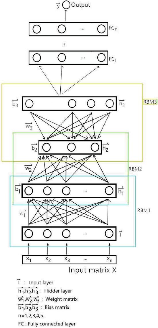
Figure 1 Model structure of IDBN-NN.

The structure of DBN proposed in this paper for renewable energy medium-term load forecasting is shown in Figure 1. It consists of an input layer, 3 hidden layers, multiple fully connected layers and an output layer. The input layer, the fully connected layer and all the hidden layers together constitute the IDBN-NN model to realize the feature extraction of the input data. The last hidden layer and the fully connected layer constitute a linear neural network, as the regression layer of the network, taking the feature vector extracted by DBN as input. The load prediction value is obtained by processing the linear activation function ReLu. To simplify the description, this article abbreviates the improved DBN network structure as IDBN-NN. Among them, the weight w1 is the symmetric connection weight between the first hidden layer h1 and the second hidden layer h2. b1 is the bias vector composed of the bias of each neuron in the first layer.

2.1 Unsupervised Training of IDBN-NN

The first part of IDBN-NN is composed of a series of RBM stacks, and the RBM training method can be used for layer-by-layer training [13]. IDBN-NN obtains the initial network parameters W and B of the load forecasting model in a complex environment through this process. The structure of RBM is shown in Figure 2. For the Bernoulli-Bernoulli RBM (BB-RBM) where both the visible unit and the hidden unit are binary random units. The values of the visible unit and the hidden unit are $I_{i} \in {0, 1}$ and $h_{j} \in {0, 1}$ , and their energy functions are as follows [16]:

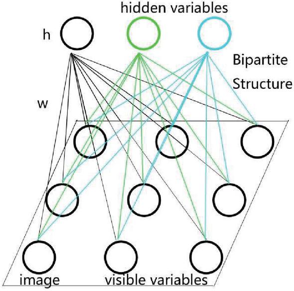
Figure 2 The model structure of RBM in DBN-NN.

In the actual renewable energy load forecasting process, due to the huge load sample size, we divide the training samples into several small batches of data sets for training in sequence. In order to improve the calculation efficiency, the weight and bias update formula for the g-th data set containing K samples can be expressed as [17]:

{\begin{matrix} w_{i j, g} = w_{i j, g - 1} + ε_{C D} [\frac{1}{K} \sum_{k = 1}^{K} (v_{i, k} h_{j, k} - v_{i, k}^{'} h_{j^{'} k}^{'})] \\ a_{i, g} = a_{i, g - 1} + ε_{C D} [\frac{1}{K} \sum_{k = 1}^{K} (v_{i, k} - v_{i, k}^{'})] \\ b_{j, g - 1} = b_{j, g - 1} + ε_{C D} [\frac{1}{K} \sum_{k = 1}^{K} (h_{j, k} - h_{j^{'} k}^{'})] \end{matrix}

(1)

In this paper, the visible unit and hidden unit are linear random unit and GB-RBM respectively. The first step is to convert the input data into binary variables through GB-RBM. The second step is to use BB-RBM for further processing. The energy function of GB-RBM is defined as [19]:

E (v, h; θ) = \sum_{i = 1}^{n} \frac{{(v_{i} - a_{i})}^{2}}{2 σ_{i}^{2}} - \sum_{i = 1}^{n} \sum_{j = 1}^{m} w i j \frac{v_{i}}{σ_{i}} h_{j} - \sum_{j = 1}^{m} b_{j} h_{j}

(2)

Where: $σ_{i}$ is the standard deviation of the Gaussian noise of visible unit $v_{i}$ . In order to simplify the calculation in the solution process, $σ_{i}$ is usually set to 1, then the formula (4) can be replaced by [19]:

P (v_{i} | h) = N (\sum_{j = 1}^{m} w_{i j} h_{j} + a_{i}, 1)

(3)

In the formula: $v_{i}$ takes the real value and obeys the Gaussian distribution with a mean of $\sum_{j = 1}^{m} w_{i j} h_{j} + a_{i}$ and a variance of 1. Except that the conditional probability distribution formula of the visible unit is different and the learning rate $ε_{CD}$ is smaller, the parameter update rule of GB-RBM is the same as that of BB-RBM.

3 Experiment

In this paper, the method of combining unsupervised training and supervised training is used to pre-train IDBN-NN [20]. When training the first layer, take x $=$ [x1, x2,…, xn] as the input vector of RBM1, and get its parameters {w1, b1} after training. In the second step, the activation probability of the hidden unit of RBM1 is used as the input vector of RBM2, and its parameters {w2, b2} are obtained according to Equation (1). The third step takes the activation probability of the hidden unit of RBM2 as the input vector of RBM3, and continues unsupervised training according to Equation (1). From this, the initial parameters of the weight W and the bias B of the IDBN-NN network can be obtained. The specific steps are shown in Figure 3.

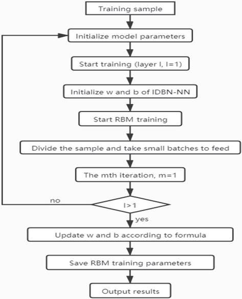
Figure 3 The entire process of IDBN-NN model training.

The mid-term load forecasting solution process of IDBN-NN is as follows. The first step is to preprocess the original data set and select the training sample set for the day to be predicted. The second step is to construct the IDBN-NN renewable energy load forecasting model, and use the training sample set to perform some supervised pre-training to obtain the initial values of the network parameters of the load forecasting model. The third step is to input the input data set at the time to be predicted into the trained IDBN-NN model after the training is completed to obtain the load prediction value at each time.

3.1 Selection of Experimental Data

The experimental sample data is based on the wind power load forecast data set of the 2012 Global Energy Forecasting Competition. According to the load characteristics of the research object power grid, the input variables of load forecasting are determined as month, week, holiday, temperature, humidity, maximum temperature, minimum temperature, average temperature, and the load of the previous 20 days.

3.2 Experimental Evaluation Index

The experimental evaluation index uses MSE, the calculation formula is as follows:

MSE = \frac{SSE}{n} = \frac{1}{n} \sum i = 1^{m} w i {(y i - y \hat{i})}^{2}

3.3 Parameter Setting and Structure Selection

In this paper, the enumeration method is used to select the number of fully connected layers and the dropout coefficient to verify the prediction effect of the deep network structure. First determine that the number of RBM layers is 3 layers. Then sequentially increase the number of fully connected layers and try the best value of the Dropout coefficient until the prediction accuracy no longer improves.

Table 1 The prediction performance of the IDBN-NN model with different structures

RBM Layers	Fully Connected Layers	Dropout Coefficient	MSE/%	Loss/%
3	1	0.1	0.31	1.36
3	1	0.2	0.37	1.04
3	1	0.3	0.56	1.05
3	2	0.1	3.2	0.85
3	2	0.2	0.83	1.16
3	2	0.3	2.44	2.44
3	3	0.1	2.11	2.19
3	3	0.2	0.54	1.05
3	3	0.3	0.53	1.43
3	4	0.1	0.42	1.02
3	4	0.2	0.53	1.36
3	4	0.3	2.39	2.43
3	5	0.1	0.32	1.41
3	5	0.2	0.46	1.53
3	5	0.3	2	2.15

Table 1 shows the respective parameters and calculation results. The value of the number of RBM layers in this article is 3. When the number of fully connected layers is 1, and the value of the Dropout coefficient is 0.1, the value of the evaluation index MSE is the smallest, 0.0031. The value of the evaluation index loss at this time is 0.0136, which is 0.0051 higher than the value of the smallest loss. When the value of the Dropout coefficient is 0.2, the value of the evaluation index MSE is 0.0037, which ranks third in the smallest value. The value of the evaluation index loss at this time is 0.0104, which is the smallest of all values. When the value of the Dropout coefficient is 0.3, the value of the evaluation index MSE is 0.0056, which is 0.0025 and 0.0019 higher than the MSE values of the former two respectively. The value of the evaluation index loss at this time is 0.0105, which is between the first two. From the above data performance, when the number of fully connected layers is 1, the value of the evaluation index MSE and the value of loss are relatively close, the change is small, and there is a certain law.

When the value of the number of fully connected layers is 2, and the value of the Dropout coefficient is 0.1, the value of the evaluation index MSE is 0.032. This value is obviously an order of magnitude higher than when the number of fully connected layers is 1. The value of the evaluation index loss at this time is 0.0085, and the loss function at this time is an order of magnitude higher than when the number of fully connected layers is 1. In this case, although the value of loss is very good, the value of MSE is relatively high. When the value of the Dropout coefficient is 0.2, the value of the evaluation index MSE is 0.0083, and the value suddenly drops again. The value of the evaluation index loss at this time is 0.0116, which is 0.0031 higher than the former. When the value of the Dropout coefficient is 0.3, the value of the evaluation index MSE and the value of loss are both 0.0244, which is worse than the two values of the first two. And it is a set of data with the worst performance when the number of fully connected layers is 2. From the above data performance, when the number of fully connected layers is set to 2, the value of the evaluation index MSE and the value of loss both change the most, and there is no certain rule.

When the number of fully connected layers is 3, when the value of the Dropout coefficient is 0.1, the value of the evaluation index MSE is 0.0211, which is relatively large and shows no signs of convergence to 0. The value of the evaluation index loss at this time is 0.0219, which is also relatively large and does not approach 0. This set of data shows that the network parameter settings at this time are not optimal, because the value of MSE and the value of loss are both large, and neither approaching zero infinitely. When the value of the Dropout coefficient is 0.2, the value of the evaluation index MSE is 0.0054, which is an order of magnitude lower than the former value. The value of the evaluation index loss at this time is 0.0105, which is 0.0114 lower than the value of the former loss. When the value of the Dropout coefficient is 0.3, the value of the evaluation index MSE is the lowest and the best among the three. The value of the evaluation index loss at this time is 0.0143, which ranks second among the three. From the performance of the above data, when the number of fully connected layers is 3, as the value of the Dropout coefficient increases, the performance of the IDBN-NN network is better.

When the number of fully connected layers is 4, when the value of the Dropout coefficient is 0.1, the value of the evaluation index MSE is 0.0042, which is relatively close to 0. The value of the evaluation index loss at this time is 0.0102, which is a relatively small value among all loss values. This set of data shows that the network is relatively stable at this time. When the value of the Dropout coefficient is 0.2, the value of the evaluation index MSE is 0.0053, which is 0.0011 higher than the former. The value of the evaluation index loss at this time is 0.0136, which is 0.0034 higher than the value of the former loss. When the value of the Dropout coefficient is 0.3, the value of the evaluation index MSE suddenly increases to 0.0239, which is the largest of the three. The value of the evaluation index loss at this time is 0.0243, which is also the largest of the three. From the performance of the above data, when the number of fully connected layers is 4, as the value of the Dropout coefficient increases, the performance of the IDBN-NN network also fluctuates greatly.

When the number of fully connected layers is 5, when the value of the Dropout coefficient is 0.1, the value of the evaluation index MSE is 0.0032, which is relatively close to 0. The value of the evaluation index loss at this time is 0.0141, which is the smallest value among the three. When the value of the Dropout coefficient is 0.2, the value of the evaluation index MSE is 0.0046, and the value at this time is closer to 0 than the former. The value of the evaluation index loss at this time is 0.0153, which is 0.0012 higher than the value of the former loss. When the value of the Dropout coefficient is 0.3, the value of the evaluation index MSE suddenly increases to 0.02, which is the largest of the three. The value of the evaluation index loss at this time is 0.0215, which is also the largest of the three. From the performance of the above data, when the number of fully connected layers is 5, as the value of the Dropout coefficient increases, the performance of the IDBN-NN network also fluctuates greatly.

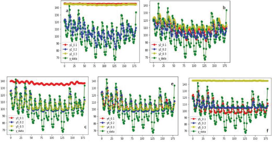
Figure 4 Load under different parameters in IDBN-NN.

It can also be seen from Figures 4a and 4c that when the number of fully connected layers is 1 and 3, the IDBN-NN network is the most stable. The value of MSE and the value of loss are also close to 0. When the number of fully connected layers is 1, the indicators of the IDBN-NN network are optimal. Figures 4b, 4d, and 4f can be seen that when the number of fully connected layers is 2, 4, and 5, as the dropout gradually increases, the IDBN-NN network begins to fluctuate.

4 Conclusion

This paper proposes a medium-term renewable energy load forecasting method based on an improved deep belief network. This method considers the renewable energy load forecasting problem affected by multiple factors in a complex environment. In the experiment, a supervised pre-training method is used to initialize the parameters of the IDBN-NN model to a better solution. Finally, the actual load data is used to analyze the calculation example. When the number of Rbm layers is 3, the number of fully connected layers is 1, and Dropout is equal to 0.2, the MSE and loss values are optimal, which are 0.0037 and 0.0104, respectively. The experimental results show that the proposed method has higher prediction accuracy when the training sample is large and the load influencing factors are complex.

References

[1] C. Q. Kang, Q. Xia, M. Liu. Power system load forecasting. Automation of Electric Power Systems, 2007, 6(16):457–467.

[2] T. Hong, P. Wang, Willis H. L. A naive multiple linear regression benchmark for short term load forecasting [C]// IEEE Power and Energy Society General Meeting, July 24–29, 2011, Detroit, USA: 1–6.

[3] Q. H. Wu, J. Jun, G. S. Hou, B. Han, K. Y. Wang. Online Recognition of Human Actions Based on Temporal Deep Belief Neural Network. Power system automation, 2016, 40(15):67–72.

[4] L. Hernandez, C. Baladron, J. M. Aguiar, et al. Artificial neural network for short-term load forecasting in distribution systems[J]. Energies, 2014, 7(3):1576–1598.

[5] J. Liu, H. Gao, M. A. Zhao. Review and prospect of active distribution system planning[J]. Journal of Modern Power Systems and Clean Energy, 2015, 3(4):457–467.

[6] T. Y. Zhou, J. Q. Yi, Y. Yang, H. T. Zhang, X. F. Yuan. Online Recognition of Human Actions Based on Temporal Deep Belief Neural Network. Acta Automatica Sinica, 2016, 15(7):1030–1039.

[7] Z. Q. Geng, Y. K. Zhang. An Improved Deep Belief Network Inspired by Glia Chains. Acta Automatica Sinica, 2016, 4(6):943–952.

[8] G. E. Hinton, S. Osindero, Y. W. Teh. A fast learning algorithm for deep belief nets[J]. Neural Computation, 2006, 18(7):1527–1554.

[9] W. Liu, Z. Wang, X. Liu. A survey of deep neural network architectures and their applications[J]. Neurocomputing, 2016, 234:11–26.

[10] Z. H. Rong, B. Qi, C. R. Li, S. J. Zhu, Y. F. Chen. Combined DBN Diagnosis Method for Dissolved Gas Analysis of Power Transformer Oil. Power System Technology, 2019, 23(10):3800–3808.

[11] J. Q. Shi, T. Tan, J. Guo, Y. Liu, J. H. Zhang. Multi-Task Learning Based on Deep Architecture for Various Types of Load Forecasting in Regional Energy System Integration. Power System Technology, 2018, 5(3):698–707.

[12] X. B. Zhang, J. Tang, C. Pan, X. X. Zhang, M. Jin. Research of Partial Discharge Recognition Based on Deep Belief Nets. Power System Technology, 2016, 40(10):3283–3289.

[13] T. Kuremoto, S. Kimura, K. Kobayashi, et al. Time series forecasting using a deep belief network with restricted Boltzmann machines[J]. Neurocomputing, 2014, 137(15):47–56.

[14] X. Qiu, L. Zhang, Y. Ren, et al. Ensemble deeplearning for regression and time series forecasting[C]// IEEE Symposium on Computational Intelligence in Ensemble Learning, December 9–12, 2014, Orlando, USA: 1–6.

[15] Dedineca, S. Filiposka, A. Dedinec, et al. Deep belief network based electricity load forecasting: an analysis of Macedonian case[J]. Energy, 2016, 115:1688–1700.

[16] G. E. Hinton. A practical guide to training restricted Boltzmann machines[J]. Momentum, 2012, 9(1):599–619.

[17] X. Y. Kong, F. Zheng, Z. J. E, J. Cao, X. Wang. Short-term Load Forecasting Based on Deep Belief Network. Power System Technology, 2018, 8(5):133–139.

[18] J. X. Zhao, X. Zhang, F. Q. Di, S. S. Guo, X. Y. Li. Exploring the Optimum Proactive Defense Strategy for the Power Systems from an Attack Perspective. Security and Communication Networks, 2021(1): 1–14.

[19] G. E. Hinton, R. R. Salakhutdinov. Reducing the dimensionality of data with neural networks[J]. Science, 2006, 313(5786):504–507.

[20] Jinxiong Zhao, Sensen Guo, Dejun Mu. DouBiGRU-A: Software Defect Detection Algorithm Based on Attention Mechanism and Double BiGRU, Computers & Security, 2021, 13(5786):504–517.

[21] You Weijing, Liu Limin, Ma Yue, et al. An Intel SGX-based Proof of Encryption in Clouds. Netinfo Security, 2020, 20(12):1–8.

[22] Xu Guotian, Shen Yaotong. A Malware Detection Method Based on XGBoost and LightGBM Two-layer Model[J]. Netinfo Security, 2020, 20(12):54–63.

[23] Li Hongjiao, Chen Hongyan. Research on Mobile Malicious Adversarial Sample Generation Based on WGAN[J]. Netinfo Security, 2020, 20(11):51–58.

[24] Guo Qiquan, Zhang Haixia. Technology System for Security Protection of Critical Information Infrastructures[J]. Netinfo Security, 2020, 20(11):1–9.

Biographies

Yan Liang (1986–), male, Han nationality, from Suide, Shaanxi, graduate degree, engineer, working in the Internet Business Department of State Grid Gansu Electric Power Company, engaged in power data management and data operation.

Li Zhi (1985–), male, Han nationality, native of Jingxian County, Anhui Province, bachelor degree, engineer, worked in the Enterprise Management Application Division of Anhui Jiyuan Software Co., Ltd. He has long been engaged in the construction of electric power information.

Yu Haiwei (1991–), male, Han nationality, native of Zibo, Shandong, bachelor degree, data analyst, working in the big data department of Hefei Maisitaihe Information Technology Co., Ltd., engaged in big data analysis and operation.

Distributed Generation & Alternative Energy Journal, Vol. 37_3, 485–500.
doi: 10.13052/dgaej2156-3306.3735
© 2021 River Publishers