A Novel Residential Energy Management System Based on Sequential Whale Optimization Algorithm and Fuzzy Logic
S. Nethravathi and Venkatakirthiga Murali*
Department of Electrical and Electronics Engineering, National Institute of Technology, Tiruchirappalli, Tamil Nadu, India
E-mail: nethrapallavi@gmail.com; mvkirthiga@nitt.edu
*Corresponding Author
Received 27 July 2021; Accepted 02 November 2021; Publication 07 December 2021
Abstract
Demand side management has become inevitable in today’s smart grid environment to balance electricity supply and demand. Many methodologies/algorithms have been developed for realizing and implementing this technique at different levels of distribution systems. Advanced metering infrastructure and the latest communication technologies have empowered residential consumers to participate in the demand side management schemes. After careful investigations and analyses, the authors of this paper have made a decisive effort to propose a novel sequential strategy for developing an energy management system for scheduling loads of residential consumers. The proposed work aims at a fuzzy logic and an evolutionary algorithm-based approach of demand side management that considers the users’ preference of operating time of the appliances at the residence of their choice, which has not been addressed earlier. This approach reduces the peak demand and cuts the cost of electricity per billing period for a consumer. This study also encourages the consumers to install solar rooftop PV systems by indicating the cost benefits reaped over a more extended period. The proposed framework is implemented in MATLAB, and the case studies prove the effectiveness of using this algorithm from the consumers’ perspective.
Keywords: Demand side management, optimization, fuzzy logic, energy management system.
1 Introduction
The ever-increasing electrical energy demand and the difficulty in satisfying the same have initiated the necessity of modifying the complete structure and protocol of operation of generation, transmission, and distribution. The smart grid envisioned as the future of power systems gives better managing capabilities both from the supplier and the consumer sides [1]. Research has proven that the smart grid is the future of energy requirements, integrating advanced sensors, communication protocols, and control technologies at transmission and distribution energy systems to distribute electricity efficiently and user-friendly. The ability to accommodate different energy generation and storage possibilities, operation based on the electric market, and user-friendliness make the smart grids more adaptable [2].
Demand Side Management (DSM) is a smart grid practice that balances demand and supply through various schemes such as time-based use, price-based use, price incentives, etc. It hence achieves a better load profile, reduced peak to average ratio (PAR), management of decentralized energy resources, bill reduction for consumers, etc. [3]. Bureau of Energy Efficiency, Ministry of Power, Government of India, states demand side management initiatives as a traditional, significant intervention to reduce energy demands while ensuring continuous development [4]. With advanced metering infrastructure (AMI) and communication facilities, DSM strategies respond actively and take action to reshape the load profile [5]. DSM implementation is beneficial for both consumers and the utility.
Broadly, DSM techniques are classified as direct load control (DLC) and indirect load control (IDLC). In DLC, the supply utility cuts off the load during peak or emergency periods. On the other hand, the IDLC scheme encourages the consumers to participate and reduce the load demand by incorporating suitable methodologies of DSM programs.
Peak clipping, valley filling, shifting of loads, strategic growth in load, strategic conservation, and flexibility in load curve are some of the DSM techniques employed. Peak clipping is where the utility uses direct load control of the consumer’s connection to grid for reducing the peak load. On the other hand, valley filling incorporates building off-peak loads. This is achieved by offering lesser price during off-peak load period and attracting the consumers to connect to the grid during off-peak period. Shifting of load involves moving loads from on-peak to off-peak period. In this method, the consumers are advised to schedule their time of use of home appliances depending on the electricity tariff. Different electricity tariffs in use are the time of usage (TOU) tariff, real-time pricing (RTP), tariff based on peak demand, etc. Strategic growth in load is encouraged by the utility to increase the sales so as to change the load-shape. In contrary, strategic conservation also changes the load-shape which is achieved by motivating the consumers to use energy efficient appliances. Flexible load curve is achieved through offering various incentives in exchange with the deviations in quality of service to the consumers [6–8].
In India, 24% of total electricity consumption is accounted for by the residential sector in 2019 and is anticipated to rise considerably in the near future, according to figures compiled by the central electricity authority (CEA) from distribution corporations [9]. Primarily driven by increased usage of appliances and apparatus, it is attributable to several factors and better access to electricity.
With the advent of smart devices and control techniques, the implementation of DSM strategies has become easier now-a-days. Residential load management has gained attention recently because of the reward obtained by implementing load control. More benefits are reaped by the consumers when combined with renewable energy sources, viz., solar photovoltaic (PV), and wind. In the recent past, detailed research has been done for developing an energy management system (EMS) for residential consumers. EMS is essentially an intelligent load management system that interfaces between the consumer and utility grid. Information such as the energy being drawn at a time or for a specified period, tariff structure if it is a variable, etc., are exchanged. EMS provides a choice-based solution to the residential consumers to effectively schedule and control the home appliances and control their energy consumption [10, 11].
Reducing PAR and the consumer bill amount are the main objectives of most of the EMSs. One significant component of EMS in achieving the goal is efficiently employing optimization algorithms. [12] proposes an automated demand response algorithm modelled as a mixed-integer nonlinear problem aiming to reduce the consumer bill by proper operation coordination among the different domestic appliances while increasing the consumers’ comfort under dynamic electricity prices. A peak management strategy is applied in [13], where the loads are shifted from peak to non-peak periods using a hierarchical decentralized algorithm. Loads that desire to receive energy sooner are given preference through the quality of service being variable. In [14], the authors propose a simple hopping scheme to lessen the peak to average ratio and retail energy price, which doesn’t require a sophisticated communication infrastructure. Three algorithms are proposed for peak reduction in smart homes, considering both consumer and utility perspectives [15]. The study also presents an incentive scheme to draw consumers’ attention to participate in the demand response program. [16] combines various operational strategies with different pricing and peak power limiting plans of a demand response program, including EV, ESS, and PV generation. Customers’ satisfaction-based HEM system is developed in [17] considering the availability of EV and distributed renewable source uncertainty.
Authors in [18] formulated the demand response program considering the electricity bill and consumer convenience as a non-convex problem under the real-time pricing paradigm is solved using a heuristic algorithm. Total energy cost is minimized by scheduling energy consumption and sharing the energy amid neighbours [19]. Minimization of energy cost is achieved by optimizing the genetic algorithm for a residential consumer considering the driving pattern of EV, degradation of the battery of EV and ESS, and supply from PV source. [20, 21] realizes a demand response strategy by utilizing EV and storage system energy bi-directionally under a peak power limiting and dynamic-pricing environment in a residential energy management system. In [22], the exchange of electricity with the grid is minimized by real-time matching between domestic loads, local renewable generation, and EV consumption using an optimization algorithm. In [10], a metaheuristic optimization solver is proposed for real-time pricing and demand charge tariff to minimize a home’s energy cost.
Recently, DSM problems are solved using the game theory approach. In [23], a real-time distributed energy management system is proposed to maintain a flat load profile for residential consumers. The solution aims to mitigate the renewable energy sources intermittency, and energy storage systems (ESS) and electric vehicles (EV) are used to supply the energy for the loads. The energy cost and peak to average ratio is relatively reduced by scheduling the residential appliances using Game theory [24].
Optimizing the consumption cost, the comfort of the end-users, and the peak to average ratio is achieved through fuzzy logic with game theory (GT) [25]. Fuzzy Inference System (FIS) combined with deep learning prediction models optimally schedule few home appliances to bring down electricity costs [26].
At this juncture, this paper proposes a novel sequential algorithm to manage four types of residential loads based on the above discussions. A nature-inspired heuristic algorithm called Whale Optimization Algorithm (WOA) is combined with Fuzzy Logic (FL) to give an optimized schedule of residential appliances. WOA is a swarm based meta-heuristic optimization algorithm which imitates the behaviour of humpback whales during hunting. The WOA algorithm is proved to be competitive by comparing the performance of 29 mathematical benchmark functions [27] with other well-known and popular meta-heuristic techniques [28–32]. The advantages of the WOA, such as better performance even with the low number of parameters, absence of local optima entrapment and faster convergence rate inspired the authors to implement the algorithm for the proposed work. Furthermore, WOA has not been applied for the DSM programs in the earlier literature to the best of the authors’ knowledge. A comparison of the literature using WOA is presented in Table 1 [33].
The paper’s novelty is that a heuristic algorithm is used to schedule the residential loads in the first stage. In the second stage, FL is used to select an optimum schedule based on the consumer’s preference of load operating time. Also, actual data is used for the study taken from a residential area load dispatch centre increasing the adaptability of the proposed work with that of the real world scenario. Specific contributions of this paper are:
• Scheduling the appliances of residential consumers according to the consumer preference using a fuzzy logic-based optimization algorithm iteratively.
• Reduction in electricity bill for the billing cycle by reducing the peak power consumed and integrating renewable energy resources for a demand-based tariff environment.
• Analysis of cost-benefit gained for various case studies and the payback period for the proposed system implementation.
• The algorithm is realized at the consumer end, and it does not require any communication with the utility, avoiding any communication errors and protecting the consumer’s confidentiality.
The rest of the paper is organized as follows: Section 2 describes the system model considered, the proposed approach and work flow. Section 3 gives the details of the input data taken for the proposed study. Section 4 deliberates the results and discussions. Finally, the conclusion is given in Section 5.
Table 1 Comparison of WOA implementation in the literature [33]
| References | Problems Addressed | Achievement |
| [34] | Optimal power flow and transient stability constrained OPF problem | Fuel cost reduction, solution quality, and convergence speed improvement |
| [35] | Maximum power point | Enhanced efficiency and accuracy by maximizing tracking speed, and energy consumption is reduced |
| [36] | Optimal sizing of DG | Reduced system loss, improved voltage profile |
| [37] | Optimal power flow problem | Better voltage profile, reduction in fuel cost, total power loss and Co2 emission |
| [38] | Economic Dispatch problem | Reduction in total fuel price |
| [39] | Optimal sizing and placement of capacitors in a radial distribution system | operating cost is reduced through stabilizing the line losses and bus voltage |
| [40] | Parameter estimation for photovoltaic cell design | Accomplished better configuration for solar cell, enhanced accuracy and robustness |
| [41] | Unit commitment Problem | Cost of power generation is reduced |
| [42] | Combined economic emission dispatch problem | Minimization of resource load, decreased fuel cost and emission value |
| [43] | Optimal power flow | Reduced fuel cost, active power loss, and reactive power loss |
| [44] | Maximum Power point tracking problem | Improvement in accuracy and speed to track global maximum power point (GMPP) |
| [45] | Optimal capacitor allocation in distribution system | Enhanced voltage profile, reduced power loss |
2 Proposed System
The test system under consideration is a locality with a group of consumers at the geographical location of 12.9425 N, 77.5626 E. There are 141 residents in the considered locality. The load consumption data of each of the consumers is collected for the study. The data collected is further grouped based on the average power demand per month.
i. The first group is where a house consumes less energy (LC).
ii. The second group of consumers consumes comparatively more energy than the first group (MC).
iii. Third group of consumers consumes high energy (HC).
iv. Fourth group has very high energy-consuming houses (VHC).
Further, the appliances of each consumer’s house are classified as:
• Schedulable Appliances (SA): These are the appliances that can be time-shifted. They do not have any constraints on the starting time. The washing machine, dishwasher, etc., belong to this category.
• Non-Schedulable Appliances (NSA): These appliances have the highest priority since they cannot be time-shifted. The appliances are switched ON as per the consumer’s desire. Light loads, fans, TV, etc., are NSAs.
• Temperature Controlled Appliances (TCA): Water heaters and air conditioners are TCAs. They can be toggled between ON/OFF when the desired temperature is met.
• Electric Vehicles (EV): These loads can perform the roles of both load and the source based on the available state of charge (SoC).
This study assumes that all the consumers are equipped with smart meter (SM) infrastructure with communication capabilities in their households. The block diagram in Figure 1 illustrates the structure of the energy management system for a single house. The Load Control Unit (LCU) receives information such as energy from the main grid, price of the energy, solar PV output available, and the consumer load data with the preferable time of operation for the appliances. The LCU is necessarily a decision-making algorithm that takes suitable action to decrease the peak demand, the overall electricity cost by suitably scheduling the loads and matching the available solar PV energy. Figure 2 demonstrates the sequential workflow followed to validate the performance of the proposed algorithm.
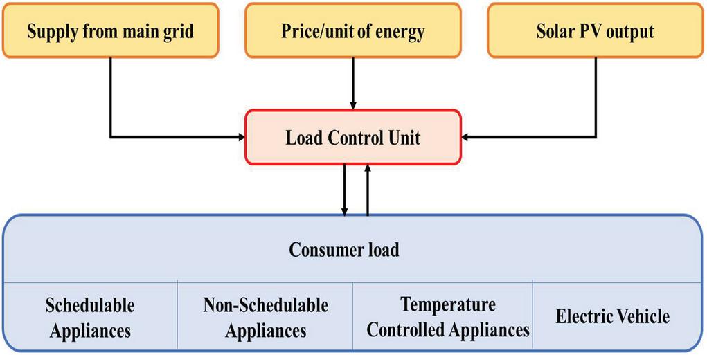
Figure 1 Block diagram of the proposed EMS.
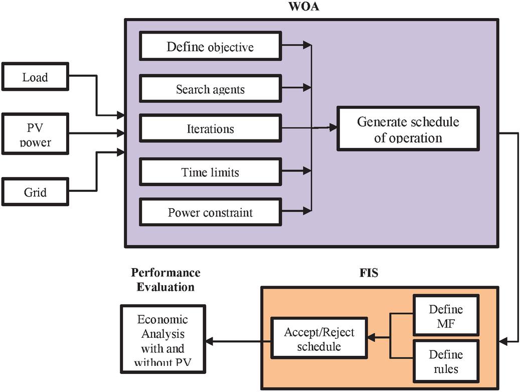
Figure 2 Experimental workflow of the proposed algorithm.
2.1 Mathematical Model Adopted
The proposed energy management strategy aims to schedule the connection time of the shiftable appliances so that the difference in the peak and Sanctioned Maximum Demand (SMD) set by the utility is reduced, resulting in a decreased electricity cost for a billing period. The billing period is a calendar month in this study. The objective function is formulated as:
| (1) |
where P SMD beyond which the consumer will be penalized
N Total number of appliances at a residence
power consumption by the nth appliance at any time t. It is given by the equation:
| (2) |
where Base Load(t) is the load present during the entire time t, Connected Load (t) is the load shifted to time t from its desired time of operation, Disconnected Load (t) is the load shifted away from time t by the LCU.
The objective function is subject to the constraints:
(i) Power balance constraint: The power drawn by the consumer should be balanced according to the equation:
| (3) |
(ii) Appliance time-shifting constraint: This constraint is based on the consumer preference for the number of time slots by which the appliance start time can be shifted. The equation representing the constraint is:
| (4) |
where T and T are the consumer-preferred time shift for the starting time of the appliance.
The Residential rooftop solar PV (RSPV) output is calculated based on the equation:
| (5) |
where:
Y PV array rated capacity under standard test conditions (STC) [kW]
f PV derating factor [%]
incident solar radiation on the PV array [kW/m]
incident radiation under STC [1 kW/m]
power temperature coefficient [%/C]
Tc PV cell temperature [C]
T temperature of PV cell under standard test conditions [25C]
Rooftop Solar Photovoltaic (RSPV) is a scheme launched by the Ministry of New and Renewable Energy (MNRE), Government of India (GoI). This scheme was introduced for residential and group housing societies with financial assistance to encourage the residential consumers to install solar PV panels on the rooftop of their residence [46]. The consumers can avail a subsidy of 40% of the benchmark cost for up to 3kW capacity solar PV installation. The capacity of the solar panel is limited to the consumer’s Sanctioned Maximum Demand (SMD). Also, the consumers can export the excess solar power to the grid and get relief from the electricity bill. If a consumer installs 1 kW capacity rooftop solar PV, the capital cost is $732.09. The subsidy of 40% received from MNRE is $292.84, and with this, the consumer investment is only $439.25.
2.2 Proposed Algorithm
In this study, a heuristic optimization algorithm called Whale Optimization Algorithm (WOA) based on whale behaviour is applied to obtain the optimal schedule of residential loads to minimize the peak power consumption and reduce the bill amount of a consumer. WOA is proven to be a very competitive algorithm compared to state-of-the-art optimization approaches [39]. The bubble net feeding method is a unique hunting method of humpback whales that WOA adapts. The prey is encircled and hunted by creating typical bubbles like a circle, spirally by the whales as shown in Figure 3(a). The same concept applies to the algorithm where the search agents move towards the optimal solution in hypercubes within the n-dimensional search space.
Humpback whales first spot the prey location and encircle them. Later whales move towards the prey in a circular fashion, every time updating their position.
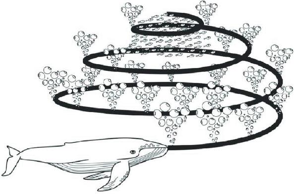
Figure 3(a) Bubble-net feeding in WOA [27].

Figure 3(b) Spiral position updating in WOA.
This behaviour is represented mathematically by the equations given as:
| (6) | |
| (7) |
where t is the present iteration, A and C are coefficient vectors, X is the vector of current position of whales, X* is the vector of the best solution obtained so far, which is replaced with better solution after each iteration. The vectors A and C are calculated as:
| (8) | ||
| (9) |
where ‘a’ is linearly reduced from 2 to 0 with every iteration and ‘r’ is a random vector in the range [0, 1].
Spiral update of position is as shown in Figure 3(b) and mathematically represented as in Equation (10):
| (10) |
where ‘p’ is a random number between [0, 1] representing the shape of logarithmic spiral, ‘l’ is between [1, 1] and ‘b’ is a constant which describes the spiral shape.
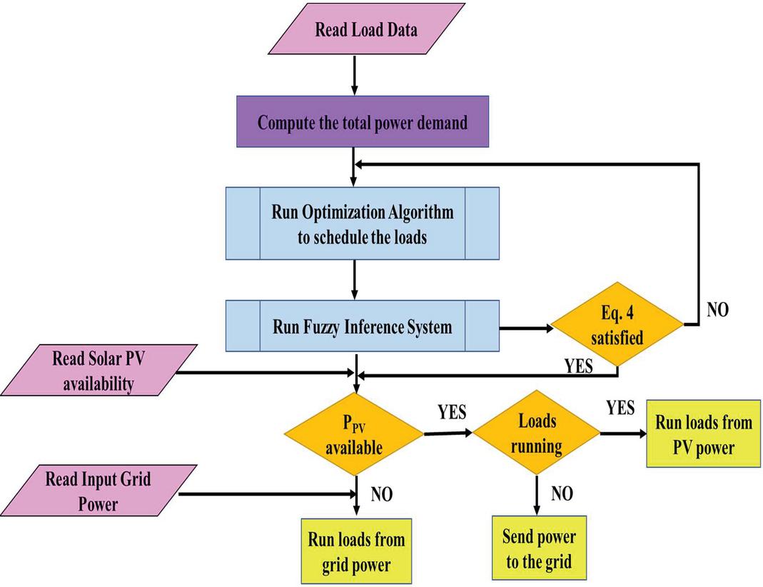
Figure 4 Flowchart for the proposed residential energy management system.
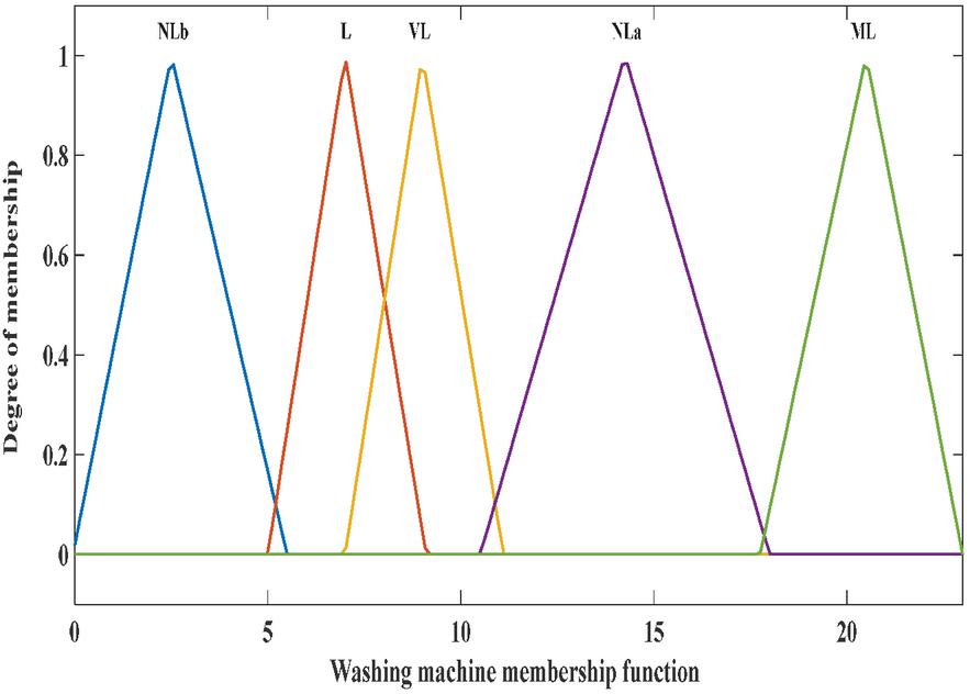
Figure 5 Membership function of washing machine.
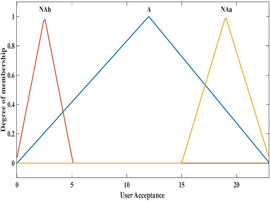
Figure 6 Output membership function.
The flowchart in Figure 4 depicts the functioning of the proposed EMS. This flowchart applies to any type of load, viz., residential and commercial loads. The inputs to the algorithm are: residential load data, available PV power, and the grid power. Based on the history of appliance usage at a residence, total power required by the connected loads at each time interval is calculated. This is fed to the WOA which schedules the loads so as to keep the total power drawn at any instant within the sanctioned maximum demand. The optimization algorithm generates time schedule of the schedulable loads based on Equation (1).
Subsequently, the schedule generated by WOA is fed into the Fuzzy Inference System (FIS), which decides whether to accept or decline the generated schedule based on the consumer preference given in Equation (4). The user preference time of operation of the appliances is modelled as fuzzy membership function and the rules are formulated. Each input is fuzzified via a triangular membership function, which describes the associated ranges of the acceptable time of operation. These are used to select the best time for the operation schedule of the appliances. Mamdani type of FIS system is used in this study [47].
The comfort level of the user to operate an appliance is represented in Figure 5 with categories, Likely (L), Very Likely (VL), Moderately Likely (ML), and two types of Not Likely (NL, NL) to reflect the degree of user acceptance regarding the selected hour to be scheduled. The output has three levels: Accepted (A) and Not Accepted (NA, NA), as shown in Figure 6. The FIS evaluates the inputs based on the If-Then rule database. The if-then rule database in this study has 75 sets of rules, representing the combination of all the six input membership degrees. This rule base includes rules which are structured as given in Table 2. Depending on the rule strength and output membership function consequence is drawn. The later decision is taken upon the defuzzification process using centroid method. This method finds the center of area of fuzzy set and returns the equivalent crisp value.
Once the acceptable schedule is generated, the algorithm checks the availability of solar power at that time interval. If the appliance operating power is lesser than the available solar power, the appliance is powered by solar. If not, as an alternative the appliance is connected to the grid. If there is a surplus solar power available, it is fed to the grid. Different case studies are analysed and presented in the subsequent section.
Table 2 Rule base of FIS implemented
| Rule # | Load 1 | Load 2 | Load 3 | Load 4 | Load 5 | Load 6 | Output |
| 1 | VL | VL | VL | VL | VL | VL | A |
| 2 | L | NL | VL | L | ML | VL | NA |
| 3 | ML | VL | L | L | VL | ML | A |
| 4 | NL | ML | L | VL | NL | L | NA |
| 75 | NL | NL | NL | NL | NL | NL | NL |
3 Simulation Study Details
3.1 Load Data
As explained in Section 2, a locality with different consumer types is validated in this study. Table 3 gives the average energy consumption/ billing cycle (month) for various types of consumers in the residential community considered.
Table 3 Average energy consumption
| Type of Consumer | Energy Consumed kWh/Month |
| VHC | 693 |
| HC | 256 |
| MC | 150 |
| LC | 80 |
VHC and HC consumers have a rooftop solar panel with a capacity of 2 kW, and MC and LC consumers have a 1 kW capacity rooftop solar panel. A scheduling range of 24 hours with a 1 hour interval period is considered for implementing the proposed work on a typical day.
3.2 Tariff and Cost of Electricity
The electricity supplied for the considered locality is Bangalore Electric Supply Company (BESCOM), Karnataka. The tariff for calculating the cost of electricity for a typical billing period is taken from [48]. BESCOM follows a demand-based tariff, which is made up of a Fixed Charge (FC) ($), and consumption Energy Charge (EC) ($/kW) is calculated based on the connected load. Fixed charges are levied based on the SMD recorded, whichever is higher, regardless of the connected load. If the recorded SMD is higher than the sanctioned load, penal charges shall apply twice the regular rate.
The Table 4 summarizes the tariff of the supply company for a residential consumer:
Table 4 Tariff for electricity
| Sanctioned Load Fixed Charge (FC) | Consumption Energy Charges (EC) | ||
| FC For 1st kW | 0.94 $ | 0 to 30 kWh | 0.054 $ |
| FC For addl. kW | 1.08 $ | 31 to 100 kWh | 0.074 $ |
| FC for EV | 0.94 $/kW | 101 to 200 kWh | 0.094 $ |
| Above 200 kWh | 0.11 $ | ||
| EV | 0.067 $/ kWh | ||
3.3 HOMER Data
The solar PV output data is obtained from Hybrid Optimization Model for Electric Renewables (HOMER) database, which is a computer model developed in 1992 by the U.S National Renewable Energy Laboratory (NREL) [49]. Daily solar irradiation on hourly basis for a day in the considered locality of this study is as shown in Figure 7, and the corresponding PV output is calculated according to Equation (5).

Figure 7 Daily Solar irradiation at the test location.
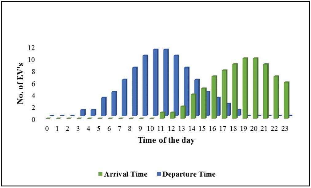
Figure 8 EV arrival and departure time.
3.4 Electric Vehicle (EV) Data
In this study, EV is considered as a load. Depending on the state of charge (SoC) available, it is used for powering the home appliances. EV arrival time is regarded as a Gaussian distribution with a mean value of 19.62 and a standard deviation of 3.62. Similarly, for departure time, the mean value is 10.53, and a standard deviation is 3.26. The data for EV is taken from [50]. Figure 8 shows the plot of EV arrival and departure time. Out of 141 consumers, 90 consumers are assumed to own EVs.
All programs are implemented in the MATLAB platform and executed on a DELL workstation. The EMS is run to obtain the day-ahead operational planning of the residential appliances.
4 Results and Discussions
The proposed work is validated for a residential locality in Bengaluru, Karnataka, considering real-time residential load data and solar irradiation. The cost of electricity for a typical month is ascertained for different scenarios. Consumers are encouraged to implement the DSM strategy by offering cost benefits for various circumstances. For this study, 6 VHC, 35 HC, 73 MC, and 27 LC homes are considered. A typical load curve for the four types of consumers considered is as shown in Figure 9.
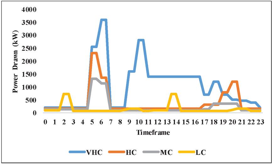
Figure 9 Load curve on regular day.
It is observed that the load exceeds the allotted SMD before applying the DSM strategy, and when every time this happens, the consumer attracts an additional charge, which is twice the regular electricity charges as given in Table 5. The proposed approach is implemented to avoid the extra costs and reduce the peak load due to excess power consumed by the connected loads. The algorithm tries to minimize the power drawn by the loads by time-shifting the schedulable loads without compromising consumer comfort. Table 4 gives the peak power drawn from the grid before and after implementing the DSM program. It is seen that there is a substantial decrease in the peak power demand.
Figure 10 depicts the number of loads that are ON at a particular time of the day before and after implementing the algorithm for VHC consumers. It is observed that the algorithm fairly distributes the number of loads connected at a given time in such a way that the peak power drawn is minimized. For instance, in Figure 10(a) there are three time periods i.e. at fifth, sixth and eighteenth hour there are five connected loads. In order to reduce the number of connected loads, the proposed algorithm pushes some of the connected loads to the time period where the number of connected loads are less in number while satisfying the consumer preference. It is seen in Figure 10(b), where the time instances mentioned above have less connected loads compared to Figure 10(a). This process is carried out for other consumers too.
Table 5 Peak reduction in power drawn from the main grid
| Without DSM (kW) | With DSM (kW) | |
| VHC | 3600 | 2600 (27.78%) |
| HC | 2300 | 1150 (50%) |
| MC | 1315 | 1140 (13.30%) |
| LC | 720 | 570 (20.8%) |
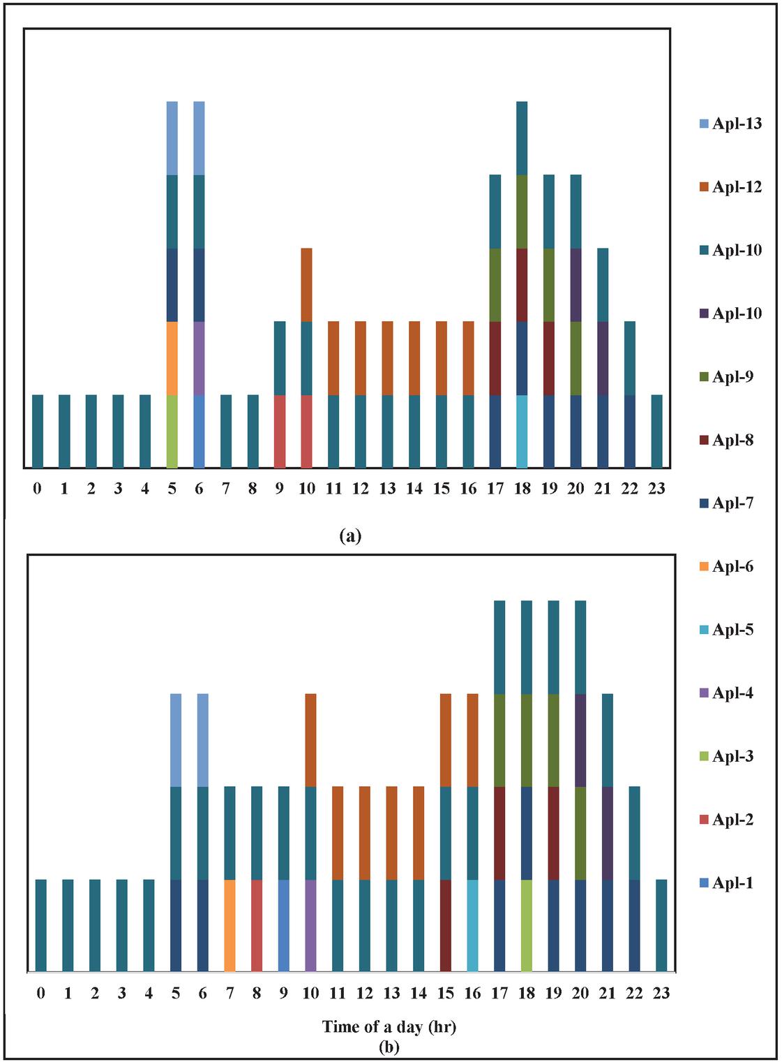
Figure 10 ON status of loads before and after scheduling for VHC consumer.
Further, when the rooftop solar is used to power the connected loads, the net power drawn further reduces, and the electricity bill is also reduced subsequently. When a consumer doesn’t want to implement any DSM but has rooftop solar for the dwelling, it still gets benefitted by reducing the power drawn from the grid and hence the cost of electricity. Figure 11 gives the load curves for all the case studies. It can be observed that there is a substantial reduction in the peak power drawn by each consumer type.
Also, with RSPV, except for the VHC consumer, the other three types of consumers are over the power required for their residential load usage at certain time intervals. This excess power is either stored as a battery backup or is sent to the grid.
BESCOM provides the consumers with the benefit of connecting solar power to its grid. For this, the consumers will be paid an amount of 0.041 $/kWh. Another case is when the consumer wants to send the entire solar-generated power to the grid and uses the power requirement by the grid alone. This case also benefits the consumer but not as much as the DSM plus PV implementation.
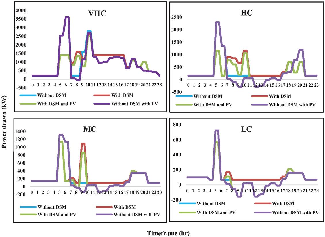
Figure 11 Load Curve for different cases under observation.

Figure 12 Cost of electricity for different cases observed.
Figure 12 shows the cost of electricity paid for a month for various case studies carried out. The cost of electricity paid to the utility and the percentage reduction compared to the base case of regular consumption without proposed algorithm implementation are summarized for each of the cases analysed in Table 6.
Table 6 Cost of electricity and percentage savings in the cost of electricity paid to the utility
| Without | Without DSM and | With | With DSM and | With DSM and | |
| DSM ($) | with PV ($) | DSM ($) | PV to Home ($) | PV to Grid ($) | |
| VHC | 169.97 | 161.31 (5.82) | 167.54 (1.49) | 157.79 (7.17) | 163.87 (3.59) |
| HC | 110.03 | 102.46 (6.94) | 108.94 (0.99) | 101.37 (7.87) | 103.92 (5.55) |
| MC | 98.08 | 94.79 (4.47) | 98.08 (0) | 93.70 (4.47) | 91.97 (6.22) |
| LC | 88.40 | 85.83 (2.9) | 88.40 (0) | 85.83 (2.9) | 82.29 (6.9) |
Figure 13 illustrates the condition when the residence is self-sustained with only PV power for the residential load. The negative value indicates that the installed RSPV power generation is over the total load requirement of the residence for a day. The generated RSPV power is stored in suitable storage systems for later use. It is observed that only VHC consumer is short of the total power required to operate the appliances for a day while other three consumers are over the power needed. For VHC consumers, a higher value of RSPV is suggested. The savings because of the extra RSPV power is also depicted in Figure 13. Since there is no excess RSPV power for VHC consumer, savings is null, whereas other types of consumers enjoy cost benefits.
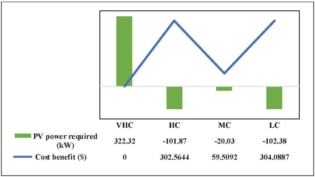
Figure 13 PV usage and savings for residence when the grid is OFF.
With the installation of RSPV, the contribution to environmental pollution is significantly reduced. In India, coal-based thermal power plants are the majority of power generators that release a considerable amount of carbon dioxide (CO). An average of 980 g of CO is released to the atmosphere by thermal power plants for one unit (kWh) of electricity generation [51]. For a VHC consumer, an average of 720 g of CO is produced for the corresponding electricity consumption of 734.7 units of energy. Installation of RSPV reduces 295.4 g of CO emission per household and, over the lifetime of the RSPV, 2953.92 g of CO emission is reduced. Figure 14 shows the emission by the thermal power plant for the required electricity usage and the corresponding reduction in emission when PV is used for fulfilling a certain amount of electricity usage for each type of household, i.e., VHC, HC, MC, and LC consumers.
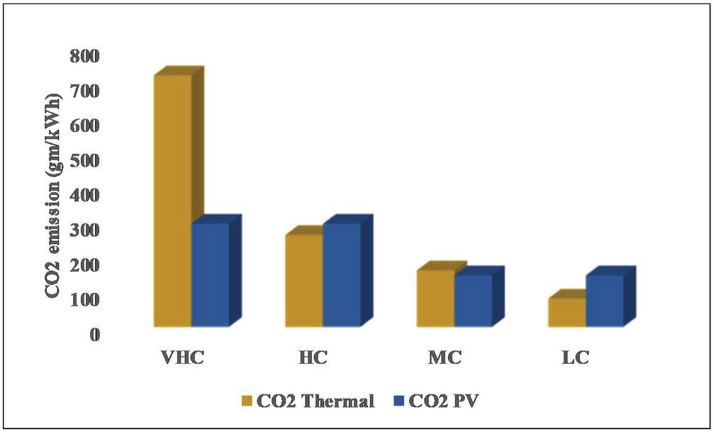
Figure 14 CO emission reduction comparison.
From the consumer point of view, the payback period is an essential factor to measure the benefits over a period of time. A simple way of calculating the payback period is attempted, based on the investment and the annual income [52], which is given as:
| (11) |
For a 1 kW RSPV installation, the total investment is 441.22 $, whereas the annual income is 20.98 $. With these values, the payback period is 7.08 years, which is significant against the lifespan of 20 years for RSPV installation. This payback period is an encouraging figure for the consumers to install RSPV, reduce power drawn from the grid, and reduce emissions.
5 Conclusion and Future Scope
This paper has presented a sequential evolutionary algorithm and fuzzy logic-based energy management system for various residential consumers in a locality of South India. Real-time data for the residential loads have been considered for the presented study. A demand-based tariff has been investigated in this work, and the consumer preference for the operation of appliances is realized using a fuzzy inference system that meets the given constraints. The cost benefits earned for different scenarios confirm the adaptability of the proposed work. In this work, load scheduling is done on the previous day, although implementing in real-time is the future work. The proposed model can be implemented practically for residential consumers, ensuring the DSM scheme’s effectiveness in a real-world application.
Authors are working on integrating the Internet of Things (IoT) and developing a graphical user interface as future work. Also, vehicle to home and vehicle to grid implementation is to be pondered.
Acknowledgements
This work has received funding from the Science and Engineering Research Board (SERB), Statutory Body Established through an Act of Parliament: SERB Act 2008, Government of India under the scheme, MATRICS, for the project titled, Internet of Energy based Interactive Residential Load Management System.
References
[1] S. Massoud Amin and B. F. Wollenberg, “Toward a smart grid: power delivery for the 21st century,” IEEE Power Energy Mag., vol. 3, no. 5, pp. 34–41, 2005, doi: 10.1109/mpae.2005.1507024.
[2] C. W. Gellings and J. H. Chamberlin, Demand-side management: Concepts and methods. United States: The Fairmont Press Inc.,Lilburn, GA, 1987.
[3] “Assessing the benefits of residential demand response in a real time distribution energy market – ScienceDirect.” https://www.sciencedirect.com/science/article/pii/S0306261915012441 (accessed Apr. 28, 2021).
[4] “No Title,” [Online]. Available: https://beeindia.gov.in/content/dsm.
[5] P. Palensky and D. Dietrich, “Demand Side Management: Demand Response, Intelligent Energy Systems, and Smart Loads,” Ind. Informatics, IEEE Trans., vol. 7, pp. 381–388, Sep. 2011, doi: 10.1109/TII. 2011.2158841.
[6] Clark W. Gellings, “The Concept of Demand-Side Management for Electric Utilities,” Proc. IEEE, no. 10, pp. 1468–1470, 1985.
[7] T. Logenthiran, D. Srinivasan, and T. Z. Shun, “Demand side management in smart grid using heuristic optimization,” IEEE Trans. Smart Grid, vol. 3, no. 3, pp. 1244–1252, 2012, doi: 10.1109/TSG.2012. 2195686.
[8] IIEC, “Demand Side Management Best Practices Guidebook for Pacific Island Power Utilities,” Strategies, no. July, 2006.
[9] “No Title,” [Online]. Available: https://cea.nic.in.
[10] F. Luo, W. Kong, G. Ranzi, and Z. Y. Dong, “Operational Dependencies,” vol. 11, no. 1, pp. 4–14, 2020.
[11] M. Pipattanasomporn, M. Kuzlu, and S. Rahman, “An algorithm for intelligent home energy management and demand response analysis,” IEEE Trans. Smart Grid, vol. 3, no. 4, pp. 2166–2173, 2012, doi: 10.1109/TSG.2012.2201182.
[12] S. Althaher, S. Member, P. Mancarella, and S. Member, “Management System Under Dynamic Pricing,” IEEE Trans. Smart Grid, vol. 6, no. 4, pp. 1874–1883, 2015.
[13] P. McNamara and S. McLoone, “Hierarchical Demand Response for Peak Minimization Using Dantzig-Wolfe Decomposition,” IEEE Trans. Smart Grid, vol. 6, no. 6, pp. 2807–2815, 2015, doi: 10.1109/TSG.2015.2467213.
[14] E. S. Parizy, H. R. Bahrami, and S. Choi, “A Low Complexity and Secure Demand Response Technique for Peak Load Reduction,” IEEE Trans. Smart Grid, vol. 10, no. 3, pp. 3259–3268, 2019, doi: 10.1109/TSG.2018.2822729.
[15] A. Jindal, M. Singh, and N. Kumar, “Consumption-aware data analytical demand response scheme for peak load reduction in smart grid,” IEEE Trans. Ind. Electron., vol. 65, no. 11, pp. 8993–9004, 2018, doi: 10.1109/TIE.2018.2813990.
[16] N. G. Paterakis, O. Erdinç, A. G. Bakirtzis, and J. P. S. Catalão, “Optimal household appliances scheduling under day-ahead pricing and load-shaping demand response strategies,” IEEE Trans. Ind. Informatics, vol. 11, no. 6, pp. 1509–1519, 2015, doi: 10.1109/TII.2015.2438534.
[17] M. Shafie-Khah and P. Siano, “A stochastic home energy management system considering satisfaction cost and response fatigue,” IEEE Trans. Ind. Informatics, vol. 14, no. 2, pp. 629–638, 2018, doi: 10.1109/TII.2017.2728803.
[18] L. Park, Y. Jang, S. Cho, and J. Kim, “Residential Demand Response for Renewable Energy Resources in Smart Grid Systems,” IEEE Trans. Ind. Informatics, vol. 13, no. 6, pp. 3165–3173, 2017, doi: 10.1109/TII.2017.2704282.
[19] S. Pal and R. Kumar, “Residential Demand Response Programs,” IEEE Trans. Ind. Informatics, vol. 14, no. 3, pp. 980–988, 2018.
[20] Y. Sun, H. Yue, J. Zhang, and C. Booth, “Minimization of Residential Energy Cost Considering Energy Storage System and EV with Driving Usage Probabilities,” IEEE Trans. Sustain. Energy, vol. 10, no. 4, pp. 1752–1763, 2019, doi: 10.1109/TSTE.2018.2870561.
[21] O. Erdinc, N. G. Paterakis, T. D. P. Mendes, A. G. Bakirtzis, and J. P. S. Catalão, “Smart Household Operation Considering Bi-Directional EV and ESS Utilization by Real-Time Pricing-Based DR,” IEEE Trans. Smart Grid, vol. 6, no. 3, pp. 1281–1291, 2015, doi: 10.1109/TSG.2014. 2352650.
[22] F. Giordano et al., “Vehicle-to-Home Usage Scenarios for Self-Consumption Improvement of a Residential Prosumer with Photovoltaic Roof,” IEEE Trans. Ind. Appl., vol. 56, no. 3, pp. 2945–2956, 2020, doi: 10.1109/TIA.2020.2978047.
[23] M. H. K. Tushar, A. W. Zeineddine, and C. Assi, “Demand-Side Management by Regulating Charging and Discharging of the EV, ESS, and Utilizing Renewable Energy,” IEEE Trans. Ind. Informatics, vol. 14, no. 1, pp. 117–126, 2018, doi: 10.1109/TII.2017.2755465.
[24] S. Pal, S. Thakur, R. Kumar, and B. K. Panigrahi, “A strategical game theoretic based demand response model for residential consumers in a fair environment,” Int. J. Electr. Power Energy Syst., vol. 97, no. January 2017, pp. 201–210, 2018, doi: 10.1016/j.ijepes.2017.10.036.
[25] M. Waseem, Z. Lin, S. Liu, Z. Zhang, T. Aziz, and D. Khan, “Fuzzy compromised solution-based novel home appliances scheduling and demand response with optimal dispatch of distributed energy resources,” Appl. Energy, vol. 290, no. February, p. 116761, 2021, doi: 10.1016/j.apenergy.2021.116761.
[26] S. Atef, N. Ismail, and A. B. Eltawil, “A new fuzzy logic based approach for optimal household appliance scheduling based on electricity price and load consumption prediction,” Adv. Build. Energy Res., vol. 0, no. 0, pp. 1–19, 2021, doi: 10.1080/17512549.2021.1873183.
[27] S. Mirjalili and A. Lewis, “The Whale Optimization Algorithm,” Adv. Eng. Softw., vol. 95, pp. 51–67, 2016, doi: 10.1016/j.advengsoft.2016. 01.008.
[28] E. Rashedi, H. Nezamabadi-pour, and S. Saryazdi, “GSA: A Gravitational Search Algorithm,” Inf. Sci. (Ny)., vol. 179, no. 13, pp. 2232–2248, 2009, doi: 10.1016/j.ins.2009.03.004.
[29] H. Li, P. G. H. Nichols, S. Han, K. J. Foster, K. Sivasithamparam, and M. J. Barbetti, “Resistance to race 2 and cross-resistance to race 1 of Kabatiella caulivora in Trifolium subterraneum and T. purpureum,” Australas. Plant Pathol., vol. 38, no. 3, pp. 284–287, 2009, doi: 10.1071/AP09004.
[30] M. F. Horng, T. K. Dao, C. S. Shieh, and T. T. Nguyen, “Advances in Intelligent Information Hiding and Multimedia Signal Processing,” Adv. Intell. Inf. Hiding Multimed. Signal Process., vol. 82, pp. 371–380, 2018, doi: 10.1007/978-3-319-50212-0.
[31] X. Yao, Y. Liu, and G. Lin, “Evolutionary programming made faster,” IEEE Trans. Evol. Comput., vol. 3, no. 2, pp. 82–102, 1999, doi: 10.1109/4235.771163.
[32] J. Kennedy and R. Eberhart, “47-Particle Swarm Optimization Proceedings., IEEE International Conference,” Proc. ICNN’95 - Int. Conf. Neural Networks, vol. 11, no. 1, pp. 111–117, 1995, [Online]. Available: http://ci.nii.ac.jp/naid/10015518367.
[33] N. Rana, M. S. A. Latiff, S. M. Abdulhamid, and H. Chiroma, Whale optimization algorithm: a systematic review of contemporary applications, modifications and developments, vol. 32, no. 20. Springer London, 2020.
[34] D. Prasad, A. Mukherjee, G. Shankar, and V. Mukherjee, “Application of chaotic whale optimisation algorithm for transient stability constrained optimal power flow,” IET Sci. Meas. Technol., vol. 11, no. 8, pp. 1002–1013, 2017, doi: 10.1049/iet-smt.2017.0015.
[35] S. Cherukuri and S. Rayapudi, “A Novel Global MPP Tracking of Photovoltaic System based on Whale Optimization Algorithm,” Int. J. Renew. Energy Dev., vol. 5, p. 225, 2016, doi: 10.14710/ijred.5.3.225-232.
[36] D. Prasad Reddy P, V. Reddy, and T. Manohar, “Whale optimization algorithm for optimal sizing of renewable resources for loss reduction in distribution systems,” Renewables Wind. Water, Sol., vol. 4, 2017, doi: 10.1186/s40807-017-0040-1.
[37] B. Bentouati, L. Chaib, and S. Chettih, “A hybrid whale algorithm and pattern search technique for optimal power flow problem,” in 2016 8th International Conference on Modelling, Identification and Control (ICMIC), 2016, pp. 1048–1053, doi: 10.1109/ICMIC.2016.7804267.
[38] H. J. Touma, “Study of The Economic Dispatch Problem on IEEE 30-Bus System using Whale Optimization Algorithm,” Int. J. Eng. Technol. Sci., vol. 3, no. 1, pp. 11–18, 2016, doi: 10.15282/ijets.5.2016.1.2.1041.
[39] D. B. Prakash and C. Lakshminarayana, “Optimal siting of capacitors in radial distribution network using Whale Optimization Algorithm,” Alexandria Eng. J., vol. 56, no. 4, pp. 499–509, 2017, doi: 10.1016/j.aej.2016.10.002.
[40] D. Oliva, M. Abd El Aziz, and A. Ella Hassanien, “Parameter estimation of photovoltaic cells using an improved chaotic whale optimization algorithm,” Appl. Energy, vol. 200, pp. 141–154, 2017, doi: https://doi.org/10.1016/j.apenergy.2017.05.029.
[41] D. Ladumor, I. Trivedi, P. Jangir, and A. Kumar, “A Whale Optimization Algorithm approach for Unit Commitment Problem Solution,” 2016, doi: 10.13140/RG.2.1.1290.2003.
[42] I. N. Trivedi, M. Bhoye, R. H. Bhesdadiya, P. Jangir, N. Jangir, and A. Kumar, “An emission constraint environment dispatch problem solution with microgrid using Whale Optimization Algorithm,” in 2016 National Power Systems Conference (NPSC), 2016, pp. 1–6, doi: 10.1109/NPSC.2016.7858899.
[43] R. H. Bhesdadiya, “Optimal Active and Reactive Power Dispatch Problem Solution using Whale Optimization Algorithm,” Indian J. Sci. Technol., vol. 9, no. 1, pp. 1–6, 2016, doi: 10.17485/ijst/2016/v9i(s1)/ 101941.
[44] N. Kumar, I. Hussain, B. Singh, and B. K. Panigrahi, “MPPT in Dynamic Condition of Partially Shaded PV System by Using WODE Technique,” IEEE Trans. Sustain. Energy, vol. 8, no. 3, pp. 1204–1214, 2017, doi: 10.1109/TSTE.2017.2669525.
[45] B. C. Neagu, O. Ivanov, and M. Gavrilaş, “Voltage profile improvement in distribution networks using the whale optimization algorithm,” in 2017 9th International Conference on Electronics, Computers and Artificial Intelligence (ECAI), 2017, pp. 1–6, doi: 10.1109/ECAI.2017.8166465.
[46] R. No, R. Energy, G. H. Societies, R. W. Scheme, C. F. Assistance, and T. Cfa, “Guidelines for Grid Connected Solar Rooftop Program under SOURA GRUHA YOJANE ( SGY ) scheme for FY,” 2020.
[47] E. H. Mamdani and S. Assilian, “An experiment in linguistic synthesis with a fuzzy logic controller,” Int. J. Man. Mach. Stud., vol. 7, no. 1, pp. 1–13, 1975, doi: 10.1016/S0020-7373(75)80002-2.
[48] K. Electricity and R. Commission, “Bangalore Electricity Supply Company Ltd.,” pp. 307–346, 2021.
[49] “How HOMER Calculates the Radiation Incident on the PV Array.”
[50] T. K. Lee, Z. Bareket, T. Gordon, and Z. S. Filipi, “Stochastic modeling for studies of real-world PHEV usage: Driving schedule and daily temporal distributions,” IEEE Trans. Veh. Technol., vol. 61, no. 4, pp. 1493–1502, 2012, doi: 10.1109/TVT.2011.2181191.
[51] S. K. Yadav and U. Bajpai, “Performance evaluation of a rooftop solar photovoltaic power plant in Northern India,” Energy Sustain. Dev., vol. 43, pp. 130–138, 2018, doi: 10.1016/j.esd.2018.01.006.
[52] V. Boddapati, A. S. R. Nandikatti, and S. A. Daniel, “Techno-economic performance assessment and the effect of power evacuation curtailment of a 50 MWp grid-interactive solar power park,” Energy Sustain. Dev., vol. 62, pp. 16–28, 2021, doi: 10.1016/j.esd.2021.03.005.
Biographies

S. Nethravathi received bachelor’s degree in Electrical and Electronics Engineering in 2005 and a master’s degree in Power Systems Engineering in 2008 from Visvesvaraya Technological University, and currently working towards a doctorate in Electrical and Electronics Engineering at National Institute of Technology Tiruchirapalli. Her research areas include demand side management, energy routing, internet of energy, and optimization techniques for energy management systems.

Venkatakirthiga Murali (M’13–SM’19) received B.E. degree in Electrical and Electronics from Bharathidasan University, Tiruchirappalli, India, in 2000, and the M.Tech. degree in Power Systems and the Doctorate degree in distributed generation and microgrids from the National Institute of Technology Tiruchirappalli (NITT), Tiruchirappalli, in 2004 and 2014, respectively. She is currently working as an Associate Professor with the Department of Electrical and Electronics Engineering, NITT. She has total teaching experience of 18 years. She is also serving as a reviewer to many reputed international journals. Her research interests include power systems, HVDC transmission systems, distribution systems, and electrical machines. She is also a Fellow Institution of Engineers, India.
Distributed Generation & Alternative Energy Journal, Vol. 37_3, 557–586.
doi: 10.13052/dgaej2156-3306.3739
© 2021 River Publishers