Power Quality Disturbance Identification and Optimization Based on Machine Learning

Fei Long^1,*, Fen Liu¹, Xiangli Peng², Zheng Yu¹, Huan Xu¹ and Jing Li³

¹State Grid Information & Communication Branch of Hubei Electric Power Co., Ltd, Wuhan 430077, China

²Hubei Central China Technology Development of Electric Power Co., Ltd, Wuhan 430000, China

³State grid Hubei Electric Power Co., Ltd, Wuhan 430070, China

E-mail: longfei436@163.com

*Corresponding Author

Received 15 June 2021; Accepted 15 July 2021; Publication 15 October 2021

Abstract

In order to improve the electrical quality disturbance recognition ability of the neural network, this paper studies a depth learning-based power quality disturbance recognition and classification method: constructing a power quality perturbation model, generating training set; construct depth neural network; profit training set to depth neural network training; verify the performance of the depth neural network; the results show that the training set is randomly added 20DB-50DB noise, even in the most serious 20dB noise conditions, it can reach more than 99% identification, this is a tradition. The method is impossible to implement. Conclusion: the deepest learning-based power quality disturbance identification and classification method overcomes the disadvantage of the selection steps of artificial characteristics, poor robustness, which is beneficial to more accurately and quickly discover the category of power quality issues.

Keywords: Power quality disturbance, deep learning, convolutional neural network.

1 Introduction

In recent years, the power quality problem increasingly prominent, and caused widespread power supply department and the general electric power users to study factors which influence the power quality, power quality decline in all sorts of problems, and realize effective classification of these problems, was very necessary to finally solve the problem of power quality and also has great realistic significance.In actual production and life, even the very short disturbance of power quality may accidentally cause inconvenience to life, production stagnation or even high recovery cost. The classification of power quality disturbance has become an important basic research topic in the field of power research in view of many unstable problems caused by it to the system and network.

In view of the serious impact of power quality decline on production and life and the wide variety of power quality phenomena, it is necessary to capture and screen power quality disturbance phenomena quickly and accurately according to the above classification method.At the same time, combined with the simulation of power quality disturbance events, a large number of data samples are generated, which lays a foundation for the in-depth study of machine learning and deep learning in the classification of power quality disturbance.

The traditional power quality analysis method includes two steps, first of all, through fourier transform, short-time fourier transform, wavelet transform, dq transform, S transform, such as digital signal processing method, characteristics of power quality disturbance are extracted, and then by artificial neural network and support vector machines, decision tree method to classify power quality disturbances. In this paper, the deep learning-based power quality disturbance identification and classification method combines the traditional method of signal analysis, feature selection and classifier construction into one, and solves the three problems through the training of deep neural network.

There are many researches on power quality disturbance identification. Lin et al. proposed a power quality disturbance recognition method based on image enhancement and feature importance analysis [1]. In order to solve the problem of noise interference in the identification of power quality disturbance, Yong et al. proposed a multi-resolution hyperbolic S-transform noise reduction method based on energy density [2]. Wang et al. proposed a DA algorithm to optimize the diagnosis of power quality disturbance and the identification of power quality disturbance model because the prediction results of extreme learning machine may be sensitive to the initial input weight and offset value [3]. Wang et al. proposed a hybrid method for feature selection and parameter optimization of complex power quality disturbance (PQD) based on S transform (ST) and immune algorithm (IA) optimization probabilistic neural network (PNN) algorithm [4]. Yang et al. proposed a complex disturbance identification method for power quality based on extremum point symmetric mode decomposition (ESMD) and support vector machine (SVM) to solve the problems of various kinds of power quality disturbances, unclear disturbance signals, many mixed disturbance phenomena and difficulty in power quality identification in actual power quality disturbances [5]. Samanta et al. proposed an automatic detection and classification method for power quality events based on stockwell transform (S transform) and WGO tuned extremum learning machine (ELM) [6]. Jian et al. established an eigenvalue evaluation system based on amplitude and phase of interference signals [7]. However, the existing digital signal processing methods are very sensitive to noise interference, and the processing time is long, so it is necessary to manually extract the features obtained from signal analysis to determine the optimal classification effect of the feature combination used, which is a cumbersome step.

Research on machine learning algorithms continues to evolve. Sun et al. compared and analyzed three popular machine learning algorithms [8]. Ling et al. proposed a slope reliability evaluation method based on machine learning, that is a multi-objective optimization multi-core limit learning machine model based on strength reduction method [9]. Singla et al. described the research progress of robust optimization in machine learning (ML), especially the research progress of support vector machine (SVM)/support vector regression (SVR) model [10].

Compared with the existing technology, based on the deep study of recognition and classification method to the traditional method of power quality disturbance signal analysis, feature selection and classifier in the building into three parts, through the depth of the training of the neural network to solve the three problems, so as to avoid the large amount of calculation of the signal analysis is sensitive to noise and other issues, this method overcomes the shortcomings of manual feature selection, such as complicated procedure and poor robustness, and is conducive to discovering the categories of power quality problems more accurately and quickly.

2 Research Methods

Experimental steps:

(1) Build a power quality disturbance model, and randomly generate several disturbance data within the parameter constraint range as the training set according to the power quality disturbance model;

(2) The deep neural network consists of a volume base layer, a pooling layer, a BN layer and a softmax layer.

(3) The training set in step (1) is used to train the deep neural network constructed in step (2) and judge whether the training index is reached. If the order judgment result is “Yes”, the next step will be entered. If the judgment result is “No”, the training will be repeated in step (3) and continue. (The training of the deep neural network adopts GPU parallel computing, the hardware is NVIDIA GTX1060 6G, and NVIDIA CUDNN package is used for acceleration.)

(4) The perturbation model in step (1) is used to generate a number of perturbation data randomly within the parameter constraint range as a test set to verify the performance of the deep neural network.If the performance meets the requirements, the trained deep neural network is used to identify and classify the power disturbance quality. Noise of 20 dB–50 dB was randomly added to the training set and verification set.

The calculation method of convolution layer is as follows:

X_{0}^{l} = f (\sum_{i \in m} X_{i}^{l - 0} \times K_{i 0}^{l} + B^{l})

(1)

The algorithm of the pooling layer adopts the maximum pooling method. The calculation formula of the maximum pooling method is as follows:

X_{0}^{l} = f (\max (\sum_{i \in m} X_{i}^{l - 1}) + B^{l})

(2)

I represents the number of network layers, K represents the convolution kernel, B represents the bias vector, $X_{o}^{l}$ represents L-layer output, $X_{i}^{l - 1}$ represents L-level input. F represents the excitation function. Further, the BN layer is used to add standardized processing to the input data of each layer in the training process of neural network. The processing method is as follows:

y_{i} = γ \times \frac{X_{i} - μ_{X}}{\sqrt{σ_{X}^{2} + ε}} + β

(3)

In the formula, $x_{i}$ is the input, $μ_{x}$ is the mean of the input x, $σ_{x}^{2}$ is the variance of the input x, $γ$ and $β$ are regular terms, ensure that the normalized output meets the standard gaussian distribution with mean 0 and variance 1.

The calculation formula of the softmax value si of the softmax layer is as follows:

S_{i} = \frac{e^{Z i}}{\sum_{1}^{j} e^{Z j}}

(4)

Si represents the probability that the input belongs to the corresponding category, and Z represents the sequence.

The calculation formula of the loss function adopted in the progressive training of the deep neural network is as follows:

l o s s = - \frac{1}{n} \sum_{i = 1}^{n} [y_{i} \ln a_{i} + (a_{i} - y_{i}) \ln (1 - a_{i})]

(5)

Yi represents the output of the deep neural network, ai represents the target output, and I represents the number of neurons in the Softmax layer.

3 Results Analysis and Discussion

3.1 Power Quality Disturbance Model

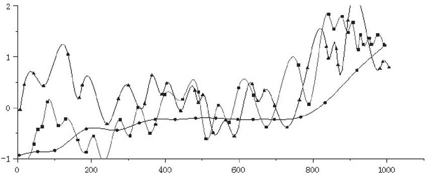
The power quality disturbance model is built as shown in Table 1. The mathematical model of the power quality disturbance sample is built based on python’s NumPy package. According to the power quality perturbation model, 768000 sets of perturbation data were randomly generated as the training set within the parameter constraint range. The generated power quality disturbance waveform is shown in Figure 1.

Table 1 Power quality perturbation model

C1	Standard signal	$y (t) = A [1 \pm α (u (t - t_{1}) - u (t - t_{2}))] \sin (w t)$	$α \leq 0.1$ $T \leq t_{2} - t_{1} \leq 9 T$
C2	Sag	$y (t) = A [1 - α (u (t - t_{1}) - u (t - t_{2}))] \sin (w t)$	$0.1 \leq α \leq 0.9$ $T \leq t_{2} - t_{1} \leq 9 T$
C3	Temporary rise	$y (t) = A [1 + α (u (t - t_{1}) - u (t - t_{2}))] \sin (w t)$	$0.1 \leq α \leq 0.8$ $T \leq t_{2} - t_{1} \leq 9 T$

Figure 1 Power quality disturbance waveform.

3.2 Deep Neural Network

The deep neural network is built based on keras, and the back-end engine adopts tensorflow. The training and subsequent experiments of the deep neural network adopt GPU parallel computing, the hardware is NVIDIA GTX1060 6G, and the CUDNN package of NVIDIA is used for acceleration.The deep neural network comprises a volume base layer, a pooling layer, a BN layer and a Softmax layer.

In essence, the convolutional layer is equivalent to a series of trainable filters, and the input data is filtered through the convolutional kernel to get the output with rich local detail features. In the image processing scene, the input is the two-dimensional pixel data stacked by the three RGB color channels, while the input of the power quality disturbance sample is the one-dimensional time series data, so the dimensions of the two-dimensional convolution layer are reduced.Let the input of the convolutional layer be a one-dimensional matrix (n $\times$ 1), where m $=$ n $-$ k $+$ 1. The calculation formula is formula (1):

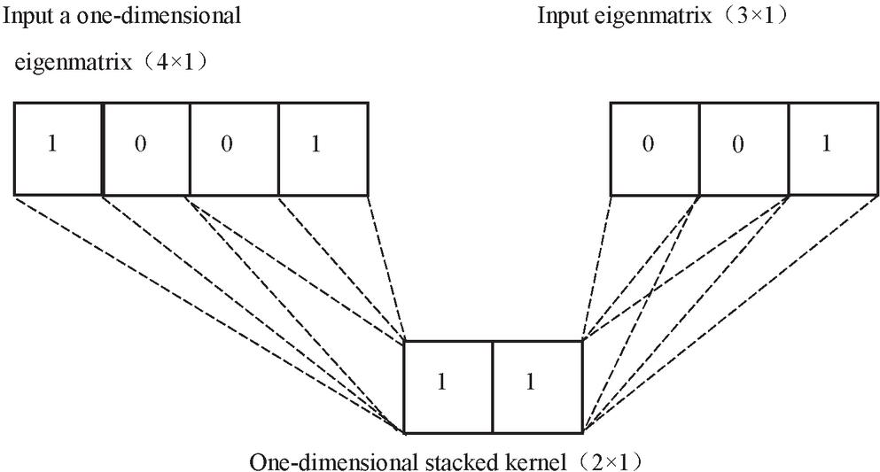
The excitation function f adopts the ReLu function, and its expression is: function f(x) $=$ Max (0,x). The one-dimensional convolution operation process is shown in Figure 2.

Figure 2 Schematic diagram of convolution operation principle.

The pooling layer is used to scale and map the convoluted data to reduce the data dimension, which can prevent overfitting to a certain extent. The pooling layer is functionally equivalent to a fuzzy filter. Common pooling methods include mean pooling, maximum pooling, etc. This embodiment adopts the maximum pool method, and the calculation formula is as follows:

X_{0}^{1} = f [\max (\sum_{i \in m} X_{i}^{l - 1}) + B^{1}]

(6)

The BN layer is used to add standardized processing to the input data of each layer in the training process of the neural network, so as to ensure that the input of each layer keeps the same distribution in the training process of the deep neural network. The introduction of BN layer can ensure the training of deep neural network at a higher learning rate, greatly improve the training speed of deep neural network, and avoid the over-fitting problem to a certain extent. Its calculation formula is formula (3):

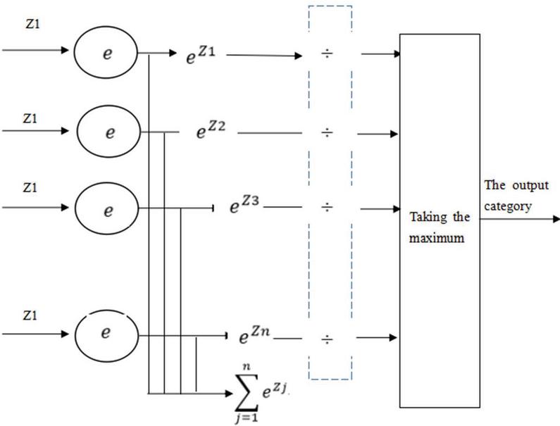
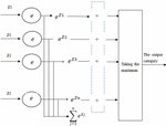
Power quality disturbance identification is a typical multi-classification problem, so softmax layer is added at the end of the network, and the number of neurons in this layer is equal to the number of category labels. For a sequence Z containing j elements, I is the subscript of Z, and Si represents the softmax value. The calculation formula is formula (4):

Si represents the probability that the input belongs to the corresponding category. The 15 neurons in the softmax layer will generate 15 softmax values corresponding to 15 candidate disturbance types. The type corresponding to the maximum value can be used to realize multi-class classification.

Figure 3 Schematic diagram of Softmax layer classification.

3.3 Training of Deep Neural Network

The training set is used to train the deep neural network constructed in 4.2 and judge whether the training index is reached. If the order judgment result is “Yes”, the next step will be entered; if the judgment result is “No”, the training will be repeated and continued.

The training of deep neural network adopts back propagation algorithm. First, the output value of the whole network is obtained through forward calculation, then the loss value between the output and the target value is calculated, and the network weight is updated in reverse to reduce the output error. This embodiment adopts category cross entropy as the loss function, and the calculation formula is formula (5):

The network weight is updated through the back propagation of the loss value. The goal of the training is to minimize the loss function value, which is realized through the optimization algorithm. The problem of solving the model parameters of deep neural network is an unconstrained optimization problem. When minimizing the loss function, it can be solved iteratively by using gradient descent method to get the minimized loss function and model parameters. There are many kinds of improved algorithm based on gradient descent, known as the optimizer, commonly used have adagrad optimizer, adadelta, RMSprop, adam. In the actual training, due to the large number of samples, it is impossible to implement the back propagation algorithm in the whole sample space, so the gradient calculation method of small batch data is adopted. In this embodiment, the number of batch training is set to 64 and NADAM is used as the optimizer, which has the advantage of realizing adaptive learning rate adjustment and efficient training.

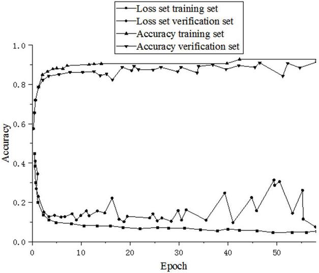
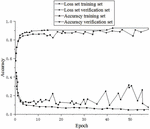
The corresponding label information in the generated data is converted into one-hot code to calculate the loss value. For example, the code ${$ 1,0,0, 0,0,0,0,0,0,0,0 $}$ represents a total of ten categories, and the sample belongs to the first category.20dB-50dB noise was randomly added to the training data to enhance the generalization performance of the model. 10% data from the training set was selected as the verification set. If no performance improvement was seen for 20 consecutive epochs on the verification set, the training would be terminated in advance. In the training stage of deep neural network, the changes of accuracy and loss values are shown in Figure 4.

Figure 4 Simulation diagram of variation process of classification accuracy and loss value.

As can be seen from Figure 4, in the training of the first 10 epochs, network performance improved rapidly. When the accuracy rate exceeded 99%, network performance improved slowly and began to show the tendency of overfitting.

3.4 Perturbation Identification Performance Test of Disturbance Model

The perturbation model in 4.1 is used to generate a number of perturbation data randomly within the parameter constraint range as a test set to verify the performance of the deep neural network. If the performance meets the requirements, the trained deep neural network is used to identify and classify the power disturbance quality.

Generate 1000 groups of test data for each disturbance type, and add noise of 40 dB, 30 dB and 20 dB respectively. The trained models were classified to test the performance of the models under different noise conditions. The test results are shown in Table 2.

Table 2 Performance of the model under different noise conditions

	Deep Convolutional Neural Network Performance

	Noise Conditions

The Disturbance Type	There is No Noise	40 dB	30 dB	20 dB
Normal waveform	100	100	98.60	97.70
Temporary rise	100	100	100	100
sag	99.7	99.70	99.70	99.20
A short interruption	100	100	99.80	99.70
flicker	100	100	100	100
FlASH $+$ TEMP	100	100	100	99.70
FlASH $+$ TEMPORARY DROP	100	100	99.90	99.50
FlASH $+$ HARMONIC	100	100	100	100
The transient oscillation	99.9	100	99.90	99.50
harmonic	100	100	100	100
Transient lift $+$ harmonic	100	100	100	100
Transient drop $+$ harmonic	100	100	100	99.80
Short interrupts $+$ harmonics	99.8	99.70	99.80	98.90
trap	100	100	100	100
The peak	100	100	100	99.90
Mean accuracy	99.96	99.96	99.85	99.59

As can be seen from Table 2, the deep neural network proposed by the invention has excellent ability to distinguish all disturbance types after repeated training of 760,000 sets of data by virtue of its strong learning ability. Thanks to the 20 dB–50 dB noise randomly added to the training set in the training process, even under the most severe 20dB noise condition, the recognition accuracy rate can still reach more than 99%, which is impossible to achieve with traditional methods. It is worth noting that, with the increase of noise signal intensity, the recognition accuracy declines most for normal waveforms. Deep neural network has a certain probability to identify normal waveforms containing gaussian noise as other disturbances, which indicates that the characteristics of normal waveforms are relatively less prominent and more vulnerable to noise pollution.

The experiment also compares deep learning with other methods in terms of recognition accuracy and anti-noise ability. The results are shown in Table 3:

Table 3 Identification accuracy and anti-noise ability of each method

			Accuracy (%)

	Number of	Identify	There
Method	Features	the Number	is No
Names	Selected	of Disturbances	Noise	40 db	30 db	20 db
Compressed sensing $+$ BP neural network	6	7	98.71	98.7	96.1	87.6
Strong tracking filter $+$ extreme learning machine	4	11	99.2	99.2	–	92.6
S transform plus the decision tree	8	13	99	99.08	99.0	91.35
Short time Fourier transform $+$ SVM	8	7	99.11	96.79	94.11	–
Change S transform $+$ direct SVM	6	11	–	96.97	94.09	91.21
Deep learning	Automatic extraction of	15	99.96	99.96	99.85	99.59

As can be seen from Table 3, the deep learning method described in this paper has absolute advantages over existing methods in terms of identification accuracy and anti-noise ability, and completely changes the traditional signal processing $+$ classifier construction analysis process, without manual participation in feature selection, which greatly reduces the difficulty of power quality disturbance modeling.

4 Conclusions

It can be seen from the analysis that the power quality disturbance recognition method based on deep learning proposed in the invention realizes the three steps of traditional signal processing, feature selection and classifier construction through a deep neural network, which simplifies the modeling steps of power quality disturbance recognition. Deep neural network integrates the advantages of feature learning of convolutional neural network, overcomes the inherent shortcomings of traditional signal processing methods, solves the problem of poor accuracy of artificial feature selection, and significantly improves the recognition accuracy and anti-noise ability. At the same time, it supports GPU parallel computing with high computing efficiency and is easy to deploy in distributed clusters, which provides favorable conditions for big data analysis of power quality disturbance.

References

[1] S Ali, K Wu, K Weston, D Marinakis. A Machine Learning Approach to Meter Placement for Power Quality Estimation in Smart Grid[J]. IEEE Transactions on Smart Grid, 7(3), pp. 1552–1561, 2016.

[2] RMA Velásquez, Lara J. Root cause analysis improved with machine learning for failure analysis in power transformers[J]. Engineering Failure Analysis, 115, p. 104684, 2020.

[3] TE Raptis, GA Vokas, PA Langouranis, SD Kaminaris. Total Power Quality Index for Electrical Networks Using Neural Networks[J]. Energy Procedia, 74, pp. 1499–1507, 2015.

[4] Tomá Vantuch, Stanislav Miák, Tomá Jeowicz, Tomá Buriánek, Václav Snáel. The power quality forecasting model for off-grid system supported by multiobjective optimization[J]. IEEE Transactions on Industrial Electronics, (12), pp. 1–1, 2017.

[5] D Xiao, F Fang, J Zheng, CC Pain, IM Navon. Machine learning-based rapid response tools for regional air pollution modelling[J]. Atmospheric Environment, 199(FEB.), pp. 463–473, 2019.

[6] MI Jordan, TM Mitchell. Machine learning: Trends, perspectives, and prospects[J]. Science, 349(6245), pp. 255–260, 2015.

[7] N Jean, M Burke, M Xie, WM Davis, S Ermon. Combining satellite imagery and machine learning to predict poverty[J]. Science, 353(6301), pp. 790–794, 2016.

[8] VUB Challagulla, FB Bastani, IL Yen, RA Paul. Empirical assessment of machine learning based software defect prediction techniques[J]. International Journal of Artificial Intelligence Tools, 17(02), pp. 389–400, 2015.

[9] ND Sidiropoulos, L De Lathauwer, X Fu, K Huang, EE Papalexakis, C Faloutsos. Tensor Decomposition for Signal Processing and Machine Learning[J]. IEEE Transactions on Signal Processing, PP(13), pp. 3551–3582, 2017.

[10] AD Vita, Z Li, JR Kermode. Molecular Dynamics with On-the-Fly Machine Learning of Quantum-Mechanical Forces[J]. Physical Review Letters, 114(9), p. 096405, 2015.

Biographies

Fei Long, born in Wuhan, Hubei Province in December 1983, graduated from Wuhan University of science and technology, obtained a master’s degree in computer software, power informatization and database technology, and a senior engineer of State Grid Information & Communication Branch of Hubei Electric Power Co., Ltd.

Fen Liu, born in March 1987 in Wuhan, Hubei Province, graduated from Wuhan University of science and technology with a master’s degree in computer software and database technology, and a senior engineer of State Grid Information & Communication Branch of Hubei Electric Power Co., Ltd.

Xiangli Peng, lives in Wuhan, Hubei Province, was born in October 1979. He graduated from Huazhong University of science and technology with a master’s degree and a senior engineer. His main research direction is computer software and database technology. At present, he works in Hubei Central China Technology Development of Electric Power Co., Ltd.

Zheng Yu, born in Wuhan, Hubei Province in December 1984, holds a master’s degree and is a senior engineer. He graduated from Huazhong University of science and technology. His main research interests are computer software, pattern recognition and intelligent system, he works in State Grid Information & Communication Branch of Hubei Electric Power Co., Ltd.

Xu Huan, born in January 1981, graduated from Huazhong University of science and technology with a master’s degree and a senior engineer. His main research interests are computer software and database technology, he works in State Grid Information & Communication Branch of Hubei Electric Power Co., Ltd.

Jing Li, live in in Wuhan in Hubei Province, born in November 1984, graduated from the school of computer software and information security of Wuhan University of science and technology, with a doctor’s degree and a senior engineer, he works in State grid Hubei Electric Power Co., Ltd.

Distributed Generation & Alternative Energy Journal, Vol. 37_2, 159–174.
doi: 10.13052/dgaej2156-3306.3723
© 2021 River Publishers