A Bionic-Intelligent Scheduling Algorithm for Distributed Power Generation System
Zhili Ma1,*, Zhenzhen Wang2 and Yuhong Zhang1
1State Grid Gansu Electric Power Company, Lanzhou 730030 China
2School of Information Science and Engineering, Lanzhou University Lanzhou 730030 China
E-mail: zhilima26@163.com; mwebemail@163.com
*Corresponding Author
Received 26 June 2021; Accepted 13 July 2021; Publication 15 October 2021
Abstract
With the introduction of the new power system concept, diversified distributed power generation systems, such as wind power, photovoltaics, and pumped storage, account for an increasing proportion of the energy supply side. Facing objective issues such as distributed energy decentralization and remote location, exploring what kind of algorithm to use to dispatch nearby distributed energy has become a hot spot in the current electric power field. In view of the current situation, this paper proposes a Bionic Intelligent Scheduling Algorithm (DWMFO) for distributed power generation systems. On the basis of the Moth Flame Algorithm (MFO), in order to solve the problem of low accuracy and slow convergence speed of the algorithm in scheduling distributed energy, we use the adaptive dynamic change factor strategy to dynamically adjust the weighting factor of the MFO. The purpose is to assist the power dispatching department to dispatch diversified distributed energy sources such as wind power, photovoltaics, and pumped storage in a timely manner during the peak power consumption period. In the experiment, we compared with 4 algorithms. The simulation results of 9 test functions show that the optimization performance of DWMFO is significantly improved, the convergence speed is faster, the solution accuracy is higher, and the global search capability is stronger. Experimental test results show that the proposed bionic intelligent scheduling algorithm can expand the effective search space of distributed energy. To a certain extent, the possibility of searching for the global optimal solution is also increased, and a better flame solution can be found.
Keywords: DWMFO, dynamic adjustment, bionic-intelligent, adaptive, distributed energy.
Introduction
With the introduction of new power system concepts, diversified distributed power generation systems such as wind power, photovoltaics, and pumped storage are taking up an increasing proportion of the energy supply side. In 1949, the total installed power generation capacity in China was 1.85 million kilowatts. In 2020, the capacity reached 2.2058 million kilowatts. In 71 years, it has increased by 1190 times. Among them, the development of clean energy power generation installed capacity is even more rapid. From a single hydroelectric power source of 160,000 kilowatts in 1949 to a multi-variety power supply “super combination” of 95.541 million kilowatts in 2020, the capacity has increased by 5971 times. Driven by the national energy strategy and policy, since 2010, China has invested about 818 billion US dollars in the field of new energy power generation, accounting for 30% of the global new energy power generation investment in the same period. As of the end of 2020, the total installed capacity of renewable energy power generation in my country reached 930 million kilowatts, accounting for 42.4% of the total installed capacity, an increase of 14.6% over 2012. Among them, the installed capacity of hydropower is 370 million kilowatts, the installed capacity of wind power is 280 million kilowatts, the installed capacity of solar power generation is 250 million kilowatts, and the installed capacity of biomass power generation is 29.52 million kilowatts. China’s clean energy power generation has increased from 680 million kilowatt-hours in 1949 to 2,449.3 billion kilowatt-hours in 2020, an increase of 3,602 times.
1 Related Research
Due to objective problems such as the scattered construction of distributed power generation systems and remote locations, most of the time, these electric energy cannot be absorbed on the spot in time. In the face of these objective problems, exploring which algorithm to use to dispatch distributed energy sources nearby has become a hot spot in the current power field. For this reason, many scholars have conducted a lot of research on the dispatching strategy of distributed energy. Aiming at the time delay problem and power loss problem of the thermal transmission network, He et al. introduced thermal delay time parameters and loss coefficients to improve the modeling accuracy of the thermal network, and studied the collaborative optimization operation of multiple energy hubs under the same energy distribution network [1]. Wang et al. proposed a multi-time-scale optimal scheduling method for integrated energy systems based on distributed model predictive control, which realizes flexible scheduling of integrated energy systems through the coordination of various subsystems [2]. Zhou et al. decomposed the topology into a three-layer system with the characteristics of “component-subsystem-main system” by introducing virtual coordinator and interconnection technology, the purpose is to facilitate the use of the target algorithm to solve the corresponding economic dispatch problem [3]. Li et al. used the second-order Taylor expansion of the original problem to make a correction to the state quantity, and used the correction result to calculate the control quantity. On this basis, an optimal power flow algorithm for distribution network with distributed energy is proposed [4]. Liu et al. applied the robust optimization method to the economic scheduling problem of electrical energy systems, and established a two-stage scheduling model with gas turbines and electric-to-gas devices as coupling components. Finally, an example is used to verify the effectiveness of the distributed robust optimization algorithm [5]. Based on the probability distribution of uncertain variables, Huang et al. used scenario analysis techniques to generate typical scenarios to fit the next day’s operating conditions and their probability of occurrence. The calculation example shows that the model improves the economy and reliability of energy supply by taking advantage of RIES’s multi-energy complementary advantages [6]. While considering diversified power generation units, Zhao et al. modeled the security of the power grid from the perspective of an attacker [7].
Although many scholars have done a lot of research on the dispatching of distributed energy sources, most of them are for the dispatching of a single energy source, and rarely consider the dispatching of three or more distributed energy sources. Aiming at the current diversified distributed energy, this paper proposes DWMFO for distributed power generation systems. Our innovation is:
(1) Diversified distributed energy sources such as wind power, photovoltaics, and pumped storage have been considered.
(2) We used the adaptive dynamic change factor strategy to dynamically adjust the weight factor of the moth flame algorithm;
(3) The experiment showed that the optimization performance of DWMFO is significantly improved, the convergence speed is faster, the solution accuracy is higher, and the global search capability is stronger.
2 Bionic Intelligent Scheduling Algorithm
2.1 Moth Flame Algorithm
2.1.1 Basic principles
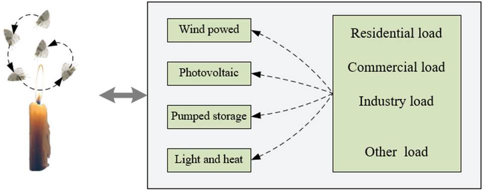
MFO is an algorithm designed to simulate the navigation mechanism of moths in the biological world. When the moth flies closer and closer to the flame, the moth will mistake the flame for the reference light. Approaching the flame at the set angle, the distance will continue to shrink, resulting in a spiral flight path, as shown in Figure 1.
Figure 1 Schematic diagram of the spiral path of the moth flame.
In the process of searching the space, the moth will update its position spirally, and the best value of the current optimal flame will be stored in the matrix.
| (1) |
In the MFO algorithm, each moth has a corresponding flame. The moths spiral toward the flame, and the algorithm does not set multiple moths to fly around a flame at the same time. The purpose is to avoid the moth from falling into the local optimum. Therefore, the dimensions of moths and flames are the same. The flame is denoted by F, and the fitness value of the flame is denoted by OF, as follows:
| (2) |
In the formula: n is the size of the population; d is the size of the dimension. The moth flame algorithm can generally be represented by a three-tuple model:
| (3) |
I represents the initialization function. In the iterative process of MFO, initial randomization of the population is carried out, and the fitness value of each moth is calculated, expressed as:
| (4) |
P represents the moth position update function. This function has very important meaning.
The operation of this function is the decision-making center of the moth update, which represents the optimization of the entire algorithm. The P function plays the role of connecting two iterations, which can be expressed as:
| (5) |
T represents the judgment condition when the operation is stopped. T will generally limit a value range, beyond the value range, the algorithm will stop running. If the conditions are met, the T function returns True; If it is not satisfied, it is False, which can be expressed as:
| (6) |
The structure of the MFO algorithm is to couple the I function, P function and T function, which can be expressed as:
The formula for the moth to update its position is expressed as follows:
| (7) | |
| (8) | |
| (9) |
Where: is the position of the i-th moth; is the j-th flame; S is the spiral function; is the distance between the flame and the moth; b is a constant; t is a random number ranging from r to 1.
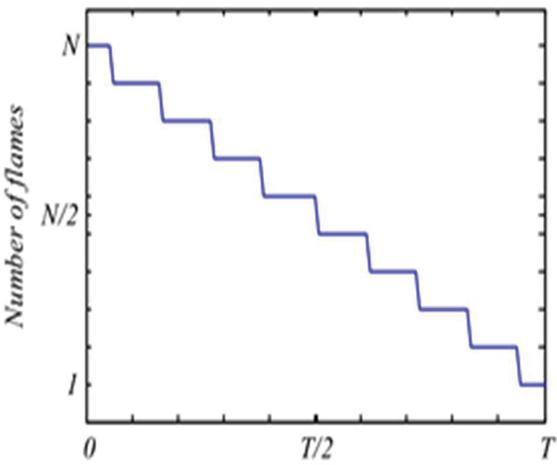
Figure 2 Iterative diagram of the number of flames.
Formula (8) has certain limitations, which makes the algorithm appear a local optimal solution. In order to make up for the existing shortcomings, the algorithm sets the flame to be adaptively reduced. The entire iterative process is shown in Figure 2 and the update formula is as follows:
| (10) |
In the formula: represents the rounded part; l is the current iteration number; N is the maximum number of flames; T is the maximum iteration number. In the calculation process, the fitness of the flame should be sorted, and the result of the sorting should follow the final elimination system.
2.1.2 Basic process
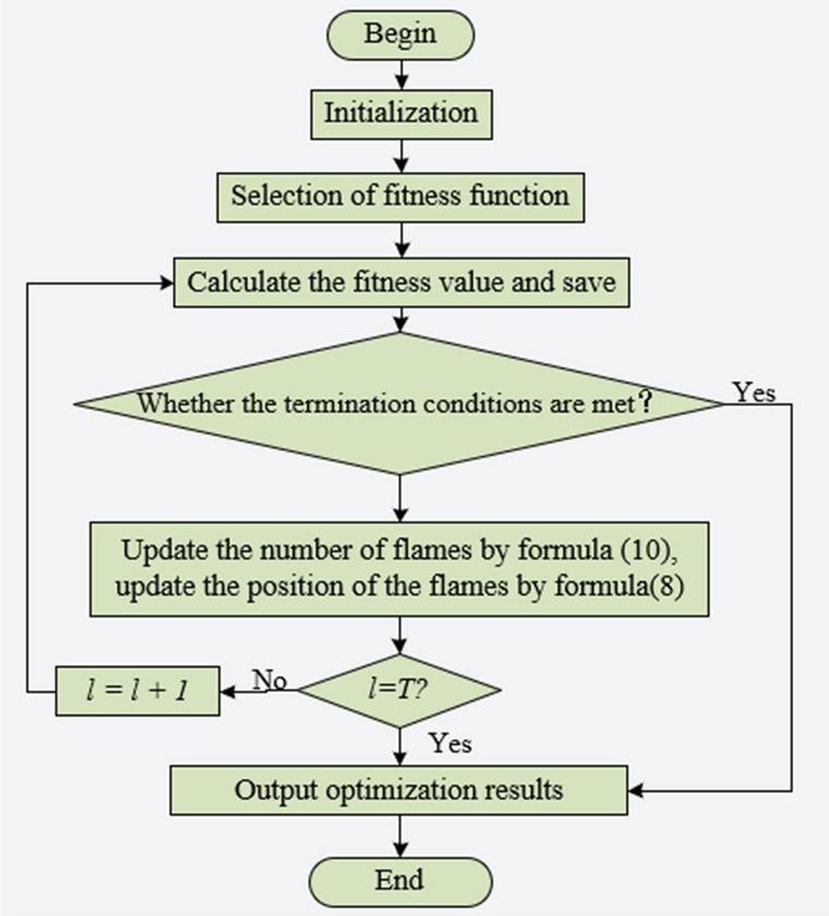
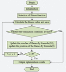
The MFO algorithm flow chart is shown in Figure 3 and the algorithm flow of MFO is as follows:
Step 1: Set the parameters, including the number of moths, the number of dimensions, and the maximum number of iterations;
Figure 3 Moth flame algorithm flow chart.
Step 2: Initialize, randomly generate moth individuals in the search space;
Step 3: Calculate the objective function corresponding to each moth, arrange the calculated results from small to large, and assign the best moth to the flame;
Step 4: Calculate the distance between the flame and the moth, and use formula (7) formula (9) to update the position of the moth;
Step 5: Use formula (10) to update the number of flames, and save the current optimal flame fitness value in the matrix;
Step 6: Increase iteration;
Step 7: Judge whether it meets the requirements for the end of the algorithm, if it does not meet the requirements, go to Step 2. Otherwise, the algorithm ends;
2.1.3 Defects in MFO algorithm
Although this algorithm can solve some practical problems, it also has some shortcomings, mainly in the following aspects:
(1) Initialization depends on randomness.
(2) The convergence speed is slow.
(3) Easy to fall into local optimum.
These shortcomings are all related to the update of its own mechanism, which leads to the poor performance of the traditional moth flame algorithm in distributed power dispatch.
2.2 Bionic Intelligent Scheduling Algorithm
In order to avoid the shortcomings of the moth flame algorithm in application, we have made two improvements to it. The first is to introduce the historical optimal flame average value of the moth flame algorithm. The purpose of this is to ensure that the information carried can expand the dimensions of information obtained by moths. Then, the adaptive dynamic change factor is introduced, the purpose of this is to prevent other moths from approaching the optimal solution of a certain local area at the same time, and to ensure that the algorithm does not fall into the local optimum.
2.2.1 Obtaining the historical optimal flame average value
In the basic MFO algorithm, the moth update formula guides the moth search through the information carried by the j-th flame. However, this can only refer to the information in one dimension, and cannot effectively use the information carried by other flames, which will cause the algorithm to slow down in the later iteration of the iteration. When this algorithm is applied to distributed power dispatching, it cannot quickly find the distributed energy source closest to the load area in a short time. Therefore, this paper introduces the concept of the historical optimal flame average, making the historical optimal flame average a factor that affects the moth’s search behavior. From a global perspective, this provides relevant information for individual moths, so that the reference information for moth search behavior is no longer limited to its own dimensions. The improved moth position update formula is as follows:
| (11) |
In formula (11), the historical optimal flame average value is introduced into the calculation of the moth flying target. The calculation formula of the average value is shown in formula (12):
| (12) |
Where: F refers to the position of the optimal flame among i historical flames of all moths, that is, the average value of the historical optimal flame. n is the number of moth i flames.
The concept of the historical optimal flame average is the use of the information carried by the optimal flame of each generation. The information carried by the historical optimal flame average can expand the dimensionality of flame-related information known by the moths. In addition, it can also guide the next movement of the moth to ensure the quality of the solution obtained by each search behavior of the moth. In this way, the moth can approach the optimal solution faster, thereby speeding up the convergence speed of the algorithm [8].
2.2.2 Introduction of adaptive dynamic factor
Due to the strong locality of the MFO algorithm, the convergence speed of the later iterations will slow down. This is the characteristic of the spiral function, and it is a problem that needs to be faced and considered. When the moth approaches the flame, it does not travel in a straight line, but approaches in a spiral. This provides greater search coverage for the basic MFO algorithm. However, this is also the case. When the moth finds a local optimal area, the spiral flight mode will cause the moth to search the local area multiple times. The optimal solution obtained by multiple searches in this area is often the local optimal solution, which causes other moths to also approach the local area. The consequence is that the algorithm falls into a local optimum. Therefore, the update method of moths is more flexible by introducing dynamic adaptive weighting factors [9]. The step size factor is changed from a fixed value to change with the increase of the number of iterations, and its dynamic change step size factor is shown in the following formula:
| (13) |
Where: l is the current number of iterations; T is the maximum number of iterations; is the logarithmic adjustment coefficient. Applying it to the logarithmic spiral function of the new moth position, it can be expressed as:
| (14) |
2.2.3 DWMFO algorithm flow
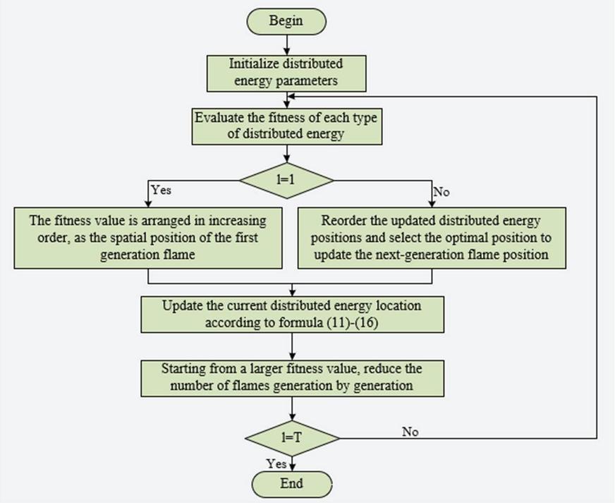
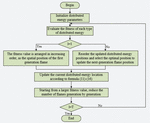
The DWMFO algorithm designed for distributed energy in this paper is as follows. We map diverse distributed energy sources such as wind power, photovoltaics, and pumped storage into different flames. The process of moths jumping into the flames is mapped to the process of dispatching diversified distributed energy by the power dispatching department. After the above mapping, solving the nearby scheduling problem actually becomes the problem of how the moth can quickly search the surrounding flames in a larger search coverage area. The historical optimal flame average corresponds to the nearest distributed energy around the local maximum load. The basic steps of the DWMFO algorithm are as follows (as shown in Figure 4):
Step 1: Parameter initialization. Set the number of distributed energy sources (such as wind power, photovoltaics, and pumped storage), the dimensionality of optimization variables, the maximum number of iterations, and the maximum number of flames;
Step 2: Initialization of distributed energy locations such as wind power, photovoltaics, and pumped storage;
Step 3: Calculate the fitness value of each type of distributed energy, sort the respective positions according to the fitness value from small to large, and find the best individual to assign to the flame;
Step 4: Use formulas (11)(15) to update the position of each distributed energy and flame;
Step 5: Record the current optimal flame fitness value;
Step 6: Reduce the number of flames according to formula (10);
Step 7: Determine whether the maximum number of iterations has been reached.
If it is reached, the optimal flame position and the corresponding fitness value in the entire iteration process are output, and the algorithm ends.
Figure 4 A bionic intelligent dispatching algorithm for distributed power generation systems.
3 Experiment
3.1 Selection of Test Function
In order to verify the optimization performance of the DWMFO algorithm, 9 test functions are selected in this paper, as shown in Table 1. At the same time, it is compared with NMFO algorithm, MFO algorithm, DEPSO algorithm, and FDMFO algorithm. In the experiment, different algorithms are run independently for 50 times, among which are unimodal functions and are multimodal functions.
Table 1 Nine test functions selected
| The | |||
| Function | Solution | Optimal | |
| Name | Function Expression | Space | Value |
| Sphere | [100, 100] | 0 | |
| Schwefel 1.2 | [100, 100] | 0 | |
| Sum square | [10, 10] | 0 | |
| Schwefel’s2.2 | [10, 10] | 0 | |
| Griewank | [600, 600] | 0 | |
| Rastrigin | [5.12, 5.12] | 0 | |
| Chaffer | [10, 10] | 0 | |
| Zakharov | [10, 10] | 0 | |
| Alpine | [10, 10] | 0 |
3.2 Test Environment and Algorithm Parameters
In the experiment, the CPU is i3-4258U 2.4GHz, the running memory is 4G, the operating system is windows8, and the programming environment is Matlab r2017. The population number of NMFO algorithm, DE algorithm, DEPSO algorithm, and GAMFO algorithm is 30, and the number of iterations is 1000. Other parameters are shown in Table 2:
Table 2 Algorithm parameter settings
| Algorithm | Parameter Settings |
| DWMFO | |
| NMFO | |
| DE | |
| DEPSO | |
| GAMFO |
3.3 Optimization Performance Analysis
Test DWMFO, NMFO [10], DE [11], DEPSO [12], GAMFO [13] algorithms on each benchmark function. The maximum number of iterations set in the experiment is 1000, and the number of distributed energy sources is 30. The calculation results are evaluated from four aspects: std (standard deviation), best (best value), mean (mean), and worst (worst value). The performance of the algorithm, the result retains four decimal places. The quality of the solution is reflected by the optimal value and the worst value. The accuracy that the algorithm can achieve is reflected by the average value. The robustness and stability of the algorithm are reflected by the standard deviation. In the experiment, the solution with the highest solution accuracy is bolded, and the function test results are shown in Table 3:
Table 3 Simulation results of all functions
| Evaluation | ||||||
| Function | Index | DWMFO | NMFO | DE | DEPSO | GAMFO |
| Sphere | std | 0 | 1.4735E-15 | 5.2772E+04 | 3.5109E+00 | 5.7202E-94 |
| best | 0 | 1.8045E-16 | 7.4888E+04 | 4.6156E+00 | 3.5470E-109 | |
| mean | 0 | 1.6138E-15 | 1.5280E+05 | 9.9220E+00 | 8.6293E-95 | |
| worst | 0 | 7.8732E-15 | 2.8809E+05 | 2.3523E+01 | 4.0465E-93 | |
| Schwefel 1.2 | std | 0 | 2.1719E-32 | 6.1169E+02 | 3.6596E-02 | 4.7694E-122 |
| best | 0 | 2.2398E-40 | 3.5117E+02 | 2.6106E-03 | 7.8741E-144 | |
| mean | 0 | 4.8853E-33 | 1.3412E+03 | 3.2228E-02 | 8.3403E-123 | |
| worst | 0 | 1.4359E-31 | 3.1714E+03 | 1.9660E-01 | 3.2869E-121 | |
| Sum | std | 0 | 2.9668E-102 | 9.4533E+00 | 4.4394E-09 | 4.3716E-146 |
| squares | best | 0 | 3.9236E-108 | 7.3992E+00 | 2.4951E-10 | 2.3624E-165 |
| mean | 0 | 1.0041E-102 | 2.1364E+01 | 3.9186E-09 | 6.1827E-147 | |
| worst | 0 | 1.5673E-101 | 5.6235E+01 | 2.0180E-08 | 3.0912E-145 | |
| Schwefel’s | std | 0 | 2.8987E-59 | 9.4533E+00 | 3.6828E-05 | 1.2598E-79 |
| problem | best | 0 | 2.3498E-63 | 7.3992E+00 | 4.9990E-06 | 1.9454E-90 |
| 2.22 | mean | 0 | 1.0715E-59 | 2.1364E+01 | 3.5684E-05 | 3.8596E-80 |
| worst | 0 | 1.7902E-58 | 5.6235E+01 | 1.8850E-04 | 6.3545E-79 | |
| Griewank | std | 0 | 1.7137E-02 | 2.3260E+00 | 4.4100E-02 | 1.2598E-79 |
| best | 0 | 0 | 2.0774E+00 | 9.8573E-03 | 1.9454E-90 | |
| mean | 0 | 1.2993E-02 | 5.7052E+00 | 8.1281E-02 | 3.8596E-80 | |
| worst | 0 | 5.4084E-02 | 1.4501E+01 | 1.7475E-01 | 6.3545E-79 | |
| Rastrigin | std | 0 | 0 | 8.5511E+00 | 1.3068E+01 | 0 |
| best | 0 | 0 | 4.1564E+01 | 2.3840E+01 | 0 | |
| mean | 0 | 0 | 6.0326E+01 | 6.4391E+01 | 0 | |
| worst | 0 | 0 | 7.8418E+01 | 8.6908E+01 | 0 | |
| Chaffer | std | 0 | 0 | 1.5338E-02 | 6.1811E-03 | 1.1717E-03 |
| best | 0 | 4.8842E-03 | 1.9038E-02 | 4.8844E-03 | 0 | |
| mean | 0 | 4.8842E-03 | 5.3128E-02 | 9.4372E-03 | 4.5912E-03 | |
| worst | 0 | 4.8842E-03 | 9.8966E-02 | 2.7695E-02 | 4.8869E-03 | |
| Zakharov | std | 0 | 9.6983E-56 | 1.6427E+01 | 8.9904E-01 | 6.0428E-123 |
| best | 0 | 1.9255E-63 | 1.8497E+01 | 2.9305E-02 | 3.0008E-144 | |
| mean | 0 | 2.8320E-56 | 4.8791E+01 | 7.2301E-01 | 9.0247E-124 | |
| worst | 0 | 6.5882E-55 | 9.2632E+01 | 4.4775E+00 | 4.2742E-122 | |
| Alipine | std | 0 | 4.6539E-06 | 1.4710E+00 | 3.9375E-02 | 6.7820E-78 |
| best | 0 | 1.0830E-60 | 2.2166E+00 | 1.7665E-06 | 3.2146E-89 | |
| mean | 0 | 1.8735E-06 | 5.6304E+00 | 9.3302E-03 | 9.6219E-79 | |
| worst | 0 | 2.8230E-05 | 9.1854E+00 | 2.4531E-01 | 4.7959E-77 |
In the experiment, 9 test functions were compared through 5 algorithms, and they were run 50 times in the same test environment. It can be seen from Table 3 that the DWMFO algorithm is much higher than the other four algorithms in terms of accuracy and stability. Whether for unimodal functions or multimodal functions with many local extreme points, the algorithm can obtain a global optimal solution. And with the change of the number of iterations, the algorithm still shows better search ability and more stable convergence performance, which shows that the improved algorithm has high solution accuracy and strong robustness. For the Sphere function, there is only one global minimum. Among them, the NMFO, GAMFO, and DEPSO algorithms [14–16] are classic improved algorithms in the algorithm, and the NMFO and GAMFO algorithms are better than DE and DEPSO in accuracy. For the Schwefel 1.2 function, the NMFO, GAMFO, and DEPSO algorithms are superior to the solution results of the DE algorithm, and the accuracy of GAMFO is 104 orders of magnitude higher than that of NMFO. For the Sum squares function, the convergence accuracy of the DE algorithm is less than that of the NMFO, GAMFO, and DEPSO algorithms. For Schwefel’s problem 2.22 function, the convergence accuracy of the four algorithms is average. For the Griewank function, the NMFO algorithm can obtain the global optimal solution. Compared with the DE, GAMFO, and DEPSO algorithms, it shows better optimization capabilities. Rastrigin is a typical nonlinear multi-modal function, it has multiple local minima, these minima ups and downs. DWMFO, NMFO, and GAMFO algorithms show significant optimization capabilities, and all of them can find the global optimum. Chaffer is a complex multimodal function. DWMFO and GAMFO algorithms show significant optimization capabilities, and both can find the global optimum. The NMFO algorithm, DE algorithm, and DEPSO algorithm cannot obtain the global optimal solution, but in terms of standard deviation, the DWMFO algorithm is better than the NMFO algorithm, which shows that the DWMFO algorithm is better than the NMFO, DE, DEPSO, GAMFO algorithm in terms of optimization stability. For Zakharov and Alipine functions, the performance of NMFO and GAMFO algorithms is better than that of DE and DEPSO algorithms.
The above results show that for 100-dimensional functions, whether it is a unimodal or multimodal function optimization problem, the search performance of the five algorithms is ranked DWMFO, GAMFO, NMFO, DEPSO, DE in order from the best to the general.
3.4 Convergence Curve Analysis
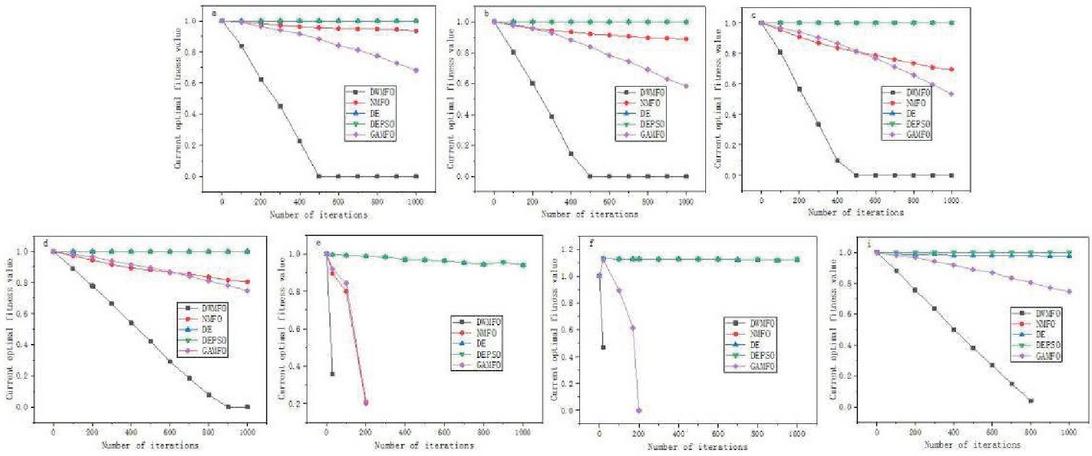
The convergence curve can visually show the convergence speed and convergence accuracy of the algorithm. Therefore, we give a comparison chart of the convergence curves of 5 algorithms under 9 functions.
Figure 5 Function convergence curve of (a) Sphere function, (b) Schwefel 1.2 function, (c) Sum squares function, (d) Schwefel’s problem 2.22 function, (e) Griewank function, (f) Rastrigin function and (i) Alipine function.
Observing the convergence curve of Figure 5(a)(i), we can see that the convergence curve of DWMFO is smooth. Compared with other four algorithms, DWMFO algorithm is better than NMFO algorithm, DE algorithm, DEPSO algorithm, GAMFO algorithm in convergence speed. After 1000 iterations, the DWMFO algorithm can converge to the global optimum, which shows that the DWMFO algorithm has a faster convergence speed and better convergence accuracy. In Figure 5(a)(d), we can see that the DWMFO algorithm has a faster convergence rate, and it overcomes the shortcomings of easy to fall into the local optimum. It is worth noting that the convergence speed of the GAMFO algorithm and the NMFO algorithm is faster than the DE algorithm and the DEPSO algorithm, and the convergence curve of the DEPSO almost coincides with the DE algorithm. Observing Figure 5(e)(f), we can find that DWMFO, NMFO, and GAMFO can converge quickly, and the convergence of DWMFO is faster than that of NMFO and GAMFO. However, the DE algorithm and the DEPSO algorithm have not converged in the iterative process. From Figure 5(g)(i), it can be found that the convergence curve of DWMFO drops rapidly to the lower left corner of the figure, especially the convergence curve of Figure 5(g) is almost close to the vertical decline, and the convergence is very fast, which is much higher than other algorithms. In summary, the DWMFO algorithm has fast convergence speed and higher convergence accuracy in dealing with high-dimensional single-mode and multi-mode problems. Its stability is higher than all other algorithms, which shows that the DWMFO algorithm has significant advantages over the other four algorithms in terms of optimization accuracy, convergence speed and solution stability.
3.5 Analysis of Operating Speed and Time Complexity
The running speed and time complexity of all algorithms also indirectly reflect the convergence speed of the algorithm. The running time of each algorithm is an important metric. Taking a single loop as an example, the DWMFO, NMFO, DE, DEPSO, and GAMFO algorithms are run speed tests on each benchmark function. The test results are shown in the table:
Table 4 Speed test results of all algorithms
| F1/s | F2/s | F3/s | F4/s | F5/s | F6/s | F7/s | F8/s | F9/s | |
| DWMFO | 0.4771 | 0.9178 | 1.2188 | 1.1330 | 1.2117 | 1.2980 | 1.2646 | 1.1873 | 1.2811 |
| NMFO | 0.4266 | 0.9091 | 1.6219 | 1.5956 | 1.5871 | 1.4994 | 1.4921 | 1.6097 | 1.5561 |
| DE | 0.2601 | 0.2282 | 0.1793 | 0.1836 | 0.1704 | 0.2429 | 0.1763 | 0.1790 | 0.1799 |
| DEPSO | 1.1012 | 1.1012 | 1.7764 | 1.8248 | 2.1175 | 1.9105 | 1.8657 | 2.0396 | 1.8469 |
| GAMFO | 0.6441 | 1.0077s | 2.0593s | 2.0486 | 2.0822 | 2.1688 | 2.0577 | 2.3464 | 2.1494 |
It can be seen from Table 4 that for single-mode functions, the DE algorithm runs the fastest, and the other four algorithms are improved compared to the DE algorithm. But DWMFO algorithm is better than NMFO, DEPSO, GAPSO algorithm. For multi-modal functions, the overall running time is longer than that of single-modal functions. The convergence speed of the DWMFO algorithm is faster than that of the NMFO, DEPSO, and GAPSO algorithms. In summary, the DWMFO algorithm has a fast convergence rate in dealing with high-dimensional single-mode and multi-mode problems. The computational complexity of the MFO algorithm depends on the number of moths n, the dimensionality of the search space d, and the maximum number of iterations T. Taking a single cycle as an example, the detailed calculation complexity is shown in Table 5:
Table 5 Comparison of time complexity of all algorithms
| Strategy | DWMFO | MFO |
| initialization | ||
| Flame selection | ||
| Number of flames | 1 | 1 |
| Parameter update | ||
| Fly towards the flame i | O(T*Number of flames) | O(T*Number of flames) |
| Flying towards the worst flame | O(n-Number of flames) | O(n-Number of flames) |
| Moths merge |
It can be seen from Table 5 that when the number of iterations of MFO and DWMFO are the same, the time complexity of each part is the same. The moth flies around the flame, and the time complexity of its MFO algorithm is:
The time complexity of the DWMFO algorithm is:
From the above analysis, it can be concluded that the time complexity of the DWMFO algorithm is the same as that of the basic MFO algorithm, which shows the advantage of the DWMFO algorithm in running time.
4 Conclusion
In this paper, aiming at the objective problems of scattered and remote location of diversified distributed power generation energy such as wind power, photovoltaic, pumped storage, etc., we introduce the historical optimal flame average value and the adaptive dynamic change factor based on the MFO algorithm, respectively. And the DWMFO algorithm for distributed power generation systems is proposed to make moths closer to the optimal solution faster, thereby accelerating the convergence speed of the algorithm. Through the verification of 9 test functions, the optimization ability, solution accuracy, and convergence speed of the DWMFO algorithm are much better than those of the other four algorithms. The simulation experiment results prove that the proposed algorithm can assist the power dispatching department to dispatch diversified distributed energy resources in a timely manner during the peak power consumption period. In the future, we will apply it in other energy fields in order to increase the robustness of the model.
References
[1] S. He, N. Liu, C. Q. Sheng, J. Y. Lei. Distributed Optimal Scheduling for Minimizing Exergy Loss Based on Joint Operation of Multiple Energy Hubs. Automation of Electric Power Systems, 2021, 9(3): 28–37.
[2] L. Wang, J. P. Zhou, L. Z. Zhu. Multi-time Scale Optimization Scheduling of Integrated Energy System Based on Distributed Model Predictive Control. Automation of Electric Power Systems, 2021, 9(3): 20–37.
[3] X. Q. Zhou, Q. Ai. Combined Distributed Robust Economic Dispatch of Distribution Network and Multiple Microgrids. Automation of Electric Power Systems, 2020, 7(2): 23–40.
[4] K. Q. Li, X. S. Han, Distributed Algorithm of Real-time Optimal Power Flow for Distribution Network with Distributed Energy Resource. Automation of Electric Power Systems, 2020, 20(1): 54–61.
[5] Y. Shui, J. Y. Liu, H. J. Gao, G. Qiu, W. T. Xu, J. Gou. Two-stage Distributed Robust Cooperative Dispatch for Integrated Electricity and Natural Gas Energy Systems Considering Uncertainty of Wind Power. Automation of Electric Power Systems, 2018, 13(3): 43–75.
[6] W. Huang, L. J. Ge, L. L. Hua, Y. B. Chen. Day-ahead Optimal Scheduling of Regional Integrated Energy System Participating in Dual Market. Automation of Electric Power Systems, 2019, 12(2): 68–82.
[7] J. Zhao, X. Zhang, F. Di, S. Guo, X. Li. Exploring the Optimum Proactive Defense Strategy for the Power Systems from an Attack Perspective. Security and Communication Networks, 2021, 2021(1): 1–14.
[8] Y. Tao, T. Huang, M. Li, et al. Research on Log Audit Analysis Model of Cyberspace Security Classified Protection Driven by Knowledge Map[J]. Netinfo Security, 2020, 20(1): 46–51.
[9] W. Luo, C. Xu. Network Intrusion Detection Based on Improved MajorClust Clustering[J]. Netinfo Security, 2020, 20(2): 14–21.
[10] C. Peng, Y. Zhao, M. Fan. A Differential Private Data Publishing Algorithm via Principal Component Analysis Based on Maximum Information Coefficient[J]. Netinfo Security, 2020, 20(2): 37–48.
[11] R. Wang, C. Ma, P. Wu. An Intrusion Detection Method Based on Federated Learning and Convolutional Neural Network[J]. Netinfo Security, 2020, 20(4): 47–54.
[12] J. Xiong, R. Bi, M. Zhao, J. Guo, Q. Yang. Edge-assisted privacy-preserving raw data sharing framework for connected autonomous vehicles, IEEE Wireless Communications, 2020, 27(3): 24–30.
[13] Y. Tian, Z. Wang, J. Xiong, J. Ma. A blockchain-based secure key management scheme with trustworthiness in DWSNs, IEEE Transactions on Industrial Informatics, 2020, 16(9): 6193–6202.
[14] D. Judhisthir, S. Rajkishore, D. Bivas. Design of Linear Phase Band Stop Filter Using Fusion Based DEPSO Algorithm, Computational Intelligence in Data Mining, 2015, 16(1): 273–281.
[15] H. Huang, H. Lei, Z. Q. Li. The Modified Temperature Field of Ceramic Roller Kiln Based on DEPSO Algorithm, Advanced Materials Research, 2011, 10(1): 1423.
[16] H. Huang, Z. H. Wei. The Back Analysis of Mechanics Parameters Based on DEPSO Algorithm and Parallel FEM, Proceedings of the 2009 International Conference on Computational Intelligence and Natural Computing, 2009, 11(1): 219–226.
Biographies

Zhili Ma, male, 38 years old, master’s degree, graduated from Lanzhou University, majoring in computer application technology, senior engineer, mainly engaged in security supervision and management and technical research. The main research directions include network security protection and intrusion detection, big data mining and analysis, Internet of Things information collection and perception.

Zhenzhen Wang (1987–), female, Han nationality, from Yicheng County, Shanxi Province. He graduated from the School of Information Science and Engineering of Lanzhou University in July 2010 with a bachelor’s degree in computer science. Since 2019, he is currently studying for a master’s degree in computer science from the School of Information Science and Engineering of Lanzhou University.

Yuhong Zhang, male, 55 years old, bachelor’s degree, graduated from Chongqing University with a major in power system automation, engineer, mainly engaged in safety supervision and management and technical research. His main research directions include power safety production big data mining analysis, safety online monitoring Internet of things, information Communication system security protection and other aspects.
Distributed Generation & Alternative Energy Journal, Vol. 37_2, 215–236.
doi: 10.13052/dgaej2156-3306.3727
© 2021 River Publishers
