Fault Detection Method of Power Insulator Based on Deep Convolution Neural Network

Yan Wang^1,* and Weijie Zhang²

¹School of Mechanical Engineering, Liaoning Technical University, Liaoning, 123000, China

²School of Electrical and Control Engineering, Liaoning Technical University, Liaoning, 125105, China

E-mail: yan_wang08@126.com; 459684561@qq.com

*Corresponding Author

Received 25 March 2021; Accepted 28 March 2021; Publication 24 June 2021

Abstract

Aiming at the problem of low detection accuracy of traditional power insulator fault detection methods, a power insulator fault detection method based on deep convolution neural network is designed. For the training of deep convolution neural network, the fault detection of power insulator based on deep convolution neural network is realized by anchor design, loss function design, candidate region selection mechanism establishment and sharing convolution features. The experimental results show that the fault detection method of power insulator based on deep convolution neural network is more accurate than the traditional method, and the detection time is less.

Keywords: Deep convolution neural network, electrical insulation, fault detection.

1 Introduction

Insulator plays an important role in electrical insulation and mechanical support of transmission line. It has been operating outdoors and in the environment for a long time. It not only bears the role of working voltage, but also bears the overvoltage caused by operation and lightning, as well as conductor weight, wind, ice and snow, dust. As well as the mechanical load effect of environmental temperature changes, the electrical performance and mechanical strength of insulators are reduced, resulting in flashover, fracture, string drop and other accidents. At present, the detection methods of the running state of the suspension insulator are as follows: (1) manual observation method, which has the advantages of heavy workload, high risk and low efficiency. (2) Ultrasonic testing method, this method is simple, high sensitivity, low cost, but due to the need for live operation, poor safety, low efficiency. (3) Laser Doppler vibration method, this method can be used to detect cracked insulators, but it is invalid to detect uncracked insulators. Although the above insulator detection methods have achieved certain results, most of them are complex operation, high cost, high risk and poor anti-interference ability.

Deep convolution neural network is a kind of feed-forward neural network. Its artificial neurons can respond to the surrounding cells in a part of the coverage area, which has excellent performance for large-scale image processing. Therefore, the deep convolution neural network is applied to the fault detection of power insulator to solve the problems existing in the current fault detection.

2 Deep Convolution Neural Network Training

2.1 Training Method

The training method of CNN is similar to BP algorithm, and the gradient descent method is generally used in back propagation. The number of samples in a single iteration of training data is divided into gradient descent (GD) for the whole training set or random gradient descent (SGD) for a single sample. The former has high complexity and low timeliness, while the latter has low complexity but unstable convergence. Therefore, there is a batch gradient descent (Mini batch SGD) between the two, and the samples of a single iteration are a subset of the random combination of the training set [1–5]. Among them, weight decay can help to avoid over fitting, and momentum can help to avoid network gradient falling into local optimum.

The training strategies of GD, SGD and Mini- Batch SGD are as follows:

$G D : w_{i + 1} = w_{i} - η_{i} \nabla_{w} L (w)$
$S G D : w_{i + 1} = w_{i} - η_{i} \nabla_{w} L (w, x_{i}, y_{i})$
$Mini - batch S G D : w_{i + 1} = w_{i} - \frac{1}{N} η_{i} \nabla_{w} L (w, x_{i}, y_{i})$	(1)

In formula (1), $w$ is the weight of the $i$ -th layer, $η$ is the learning rate, and $L$ is the loss function.

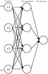
The whole training process is divided into forward propagation and reverse propagation. The detailed description of each part is shown in Figure 1:

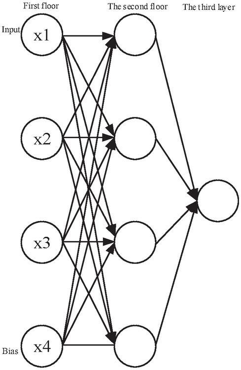
Figure 1 Neural network model.

In the forward propagation process, the output value of the activation function of each neuron in each layer is calculated after the given sample set. Then, the output value of the whole network can be obtained in the last layer according to the hierarchy, the expression is as follows:

J (W, b) = [\frac{1}{m} \sum_{m}^{i = 1} J (W, b; x^{(i)}, y^{(i)})] + \frac{l}{2} \sum_{m - 1}^{l = 1} \sum_{s l}^{i = 1} \sum_{s i + l}^{j = 1} {(W_{j i}^{(i)})}^{2}

(2)

In formula (2), $J (W, b)$ is composed of mean square error term and regularization term. Regularization is added to punish neurons with heavy weights, and the over fitting is reduced by reducing the amplitude of neuron weights [6–10]. In the batch gradient descent method, the weight matrix of neural network is updated according to the following formula at each iteration, the expression is as follows:

W_{i j}^{(b)} = W_{i j}^{(l)} - α \frac{\partial}{\partial W_{i j}^{(l)}} J (W, b)

(3)

In formula (3), $\partial$ is the learning rate, $b$ is the bias, and $W$ is the weight matrix.

2.2 Regularization Method

In the process of training, the common problems are over fitting and under fitting. The over fitting performance is that the accuracy of the model is very high in the training set, but not ideal in the test set. Under fitting results are not ideal. Because the deep neural network contains a large number of parameters, over fitting often occurs. This is due to the small size of the training data set, the complexity of the model, the limited computing resources and the existence of noise.

2.3 Pre Training and Fine Tuning

The models of deep learning are multi-layer, even hundreds of layers. If the whole network is trained at the same time, the convergence of the network is too slow due to too many layers and parameters. If the training is carried out layer by layer, the error will pass down in turn and become larger and larger. This is because the gradient will be more and more sparse with the depth direction of the network during training, and the error correction signal will be smaller and smaller. Finally, the network is easy to converge to the local minimum during random initialization.

Hinton put forward the idea of pre training and fine-tuning network, first the bottom-up unsupervised learning, and then the top-down supervised learning. For many applications, only a small amount of training data is available. Convolutional neural networks usually need a lot of training data to avoid over fitting. Since the input of the fine tuned network is obtained in the pre training rather than random initialization, it is closer to the global optimal value. Fine tuning the network allowing convolution can successfully solve the engineering problem of small training set.

2.4 Determination of Topological Structure of Neural Network

It is generally believed that increasing the number of hidden layers can reduce the network error and improve the accuracy, but it also complicates the network, thus increasing the network training time and the tendency of “over fitting”. Hornik et al. have proved that if the input layer and output layer adopt linear transfer function, and the hidden layer adopts sigmoid transfer function, the MLP network with one hidden layer can approximate any rational function with any precision. When designing BP network, three-layer BP network (i.e. one hidden layer) should be given priority. Generally, it is easier to get lower error by increasing the number of hidden layer nodes than by increasing the number of hidden layer nodes. Based on this, this paper selects a three-layer structure of neural network.

In order to avoid “over fitting” phenomenon in training and ensure high enough network performance and generalization ability, the basic principle of determining the number of hidden layer nodes is to select as compact a structure as possible on the premise of meeting the accuracy requirements, that is, to select as few hidden layer nodes as possible. When determining the number of hidden layer nodes, the following conditions must be satisfied:

(1) The number of hidden nodes must be less than that of otherwise, the system error of network model is not related to the characteristics of training samples and tends to zero;

(2) The number of training samples must be more than the connection weights of network model, generally 2–10 times.

The number of hidden layer elements can be calculated according to the formula:

n^{\circ} = \sqrt{m + n} + a

(4)

In formula (4), $m$ is input neuron and $n$ is output neuron.

(3) In the standard gradient descent algorithm, the iterative formula of weight is as follows:

w_{i j} (n + 1) = w_{i j} (n) + η [(1 - α) D (n) + α D (n - 1)]

(5)

This method has one disadvantage: the learning rate is fixed in the training process. If the learning rate is set too high, there may be oscillation and instability in the training process; if the learning rate is set too low, the convergence time will be too long. In this paper, a gradient descent algorithm with variable learning rate is used. The design criteria are: check whether the weight really reduces the error function; if so, it indicates that the selected learning rate is small and can be increased by an appropriate amount; if not, the value of learning rate should be reduced [11–15]. An adaptive learning rate adjustment formula is given by the following formula:

η (k + 1) = {\begin{matrix} 1.05 η (k) & E (k + 1) < E (k) \\ 0.7 η (k) & E (k + 1) > 1.04 E (k) \\ η (k) & e l s e \end{matrix}

(6)

In formula (6), $E (k)$ represents the sum of squares of the $k$ -th error.

3 Fault Detection of Electronic Insulator Based on Deep Convolution Neural Network

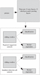
The method is mainly composed of two parts: the first part is a full convolution neural network used to generate a series of efficient candidate regions, which is called region proposal network (RPN); the second part is a fast R-CNN network used to determine the specific location of insulators. The weight parameters and characteristics of the two parts are shared, so that it does not need to spend more time to do repeated calculation in the insulator detection stage, which can greatly reduce the amount of calculation of the network.

Region recommendation network can process insulator input image of any size, and then output a series of regions of interest with rectangular box, and each region of interest belongs to the confidence of a target. Next, we mainly discuss how to model regional recommendation networks and how to generate efficient regions of interest [16–20]. The algorithm framework is shown in Figure 2.

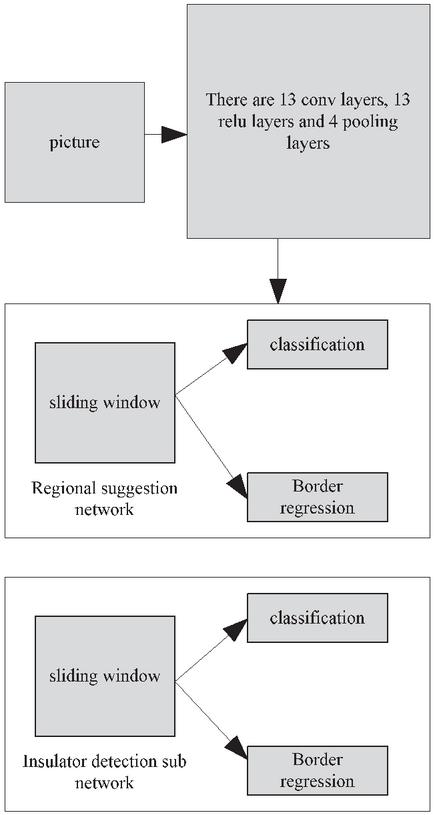
Figure 2 Algorithm framework.

The convolution neural network used in this chapter is VGG16 network, which consists of 13 convolution layers and 4 pooling layers. In the process of generating candidate region, the insulator image is sent to VGG16 network, and the feature extraction and dimension reduction are carried out continuously through the convolution layer and pooling layer. 512 feature maps are output in the last convolution layer. After obtaining the feature, we add a small network to slide on the feature map. The network takes n * n input from convolution feature graph, maps the feature corresponding to each sliding window to a lower dimension (512 dimension), and then uses ReLU to do nonlinear processing. Then, the features are sent into two fully connected layers, one is used for border regression, and the other is used to judge whether the framed area belongs to the target area.

3.1 Anchor Point

In the position of each sliding window, it is necessary to determine whether multiple interested areas contain insulator targets at the same time. We will record the number of areas predicted at each location as K. For this k region, the border regression layer outputs 4K coordinates and the classification layer outputs 2K confidence scores. Here, k-region parameterization is associated with K reference boxes, which are called anchor points.

In this process, the center of the sliding window is the center of the anchor point, and regions with different scales and length width ratios are selected around the center. According to the shape characteristics of the insulator, we choose the pixel area of 1282,2562,5122 and the aspect ratio of 1:1, 1:4, 4:1, and each center corresponds to 9 anchor points. For a W * H feature image, there are k-WH anchors.

3.2 Loss Function

When anchors in the training regional recommendation network, each anchor point is need to be assigned a binary label (insulator or not). Among them, the anchor points meeting one of the following two conditions are designated as positive samples: (1) the anchor points with the maximum division and overlap ratio (Io U) of an insulator marker box; (2) the anchor points with the division and overlap ratio of any insulator marker box exceeding 0.7. In the actual insulator image, a single insulator label box may assign positive labels to multiple anchors. Anchor points with Io U less than 0.3 of all insulator marker frames in the image are assigned as negative labels. Those anchors that are neither set as negative tags nor assigned positive tags will be screened out and will not participate in network training [21–25].

On the basis of label assignment, we need to minimize the multi task loss function in the process of training model. For an insulator image, the loss function is defined as follows:

L = \frac{1}{N_{c h}} \sum_{i} L_{c b} (q_{i}, q_{i}^{*}) + α \frac{1}{N_{r e g}} \sum_{i} q_{i}^{*} L_{r e g} (t_{i}, t_{i}^{*})

(7)

In formula (7), $q_{i}$ represents the probability of prediction as the target, $α$ represents the equilibrium coefficient, $L_{r e g}$ is the logarithmic loss function of two categories (target and non target), $L_{c b}$ represents the regression loss function.

In order to correct the boundary frame of insulator, the parameterization of four coordinates should be adopted:

$t_{x}$	$= \frac{x - x_{a}}{w_{a}}, t_{y} = \frac{y - y_{a}}{h_{a}}$
$t_{w}$	$= \log (\frac{w}{w_{a}}), t_{h} = \log (\frac{h}{h_{a}})$
$t_{x}^{*}$	$= \frac{x^{} - x_{a}}{w_{a}}, t_{y}^{} = \frac{y^{*} - y_{a}}{h_{a}}$
$t_{w}^{*}$	$= \log (\frac{w^{}}{w_{a}}), t_{h}^{} = \log (\frac{h^{*}}{h_{a}})$	(8)

In the formula, $x, y, z$ is the center coordinates, length and width of the prediction box, $x_{a}, y_{a}, w_{a}$ is the center coordinates, length and width of the candidate area box, and $x^{*}, y^{*}, w^{*}$ is the center coordinates, length and width of the real box.

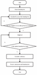
3.3 Candidate Region Selection Mechanism

The selection process of candidate region selection mechanism is shown in Figure 3:

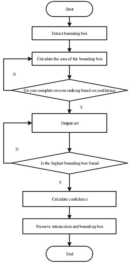
Figure 3 Working process of candidate region selection mechanism.

After the candidate regions are obtained by using the region recommendation network, the candidate regions need to be mapped to the last convolution layer, and then the corresponding features of each candidate region are sent to the ROI pooling layer and the full connection layer. Finally, the classification layer is used to determine whether the candidate region is a target, and the border regression layer is used to adjust the border to make the target position more accurate. In the process of training Fast R-CNN network, the candidate regions whose ratio of intersection and union of insulator real regions is greater than or equal to 0.5 are regarded as positive samples, and the rest are regarded as negative samples. When training the network, the multi task loss function shown in the following formula is selected:

L (p, u, t^{''}, v) = L_{c l s} (p, u) + α .

(9)

In formula (9), $u$ is the label of insulator, $L_{c l s}$ and $L_{l o c}$ are the classification loss function and the frame regression loss function respectively. $t^{μ}$ and $v$ represent the four coordinate values of prediction frame and real insulator frame respectively.

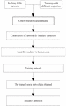
3.4 Shared Convolution Feature

When two networks are trained, there is a part of convolution layer feature sharing. In this paper, we use 4-stage alternating training to optimize the shared convolution features. The process is shown in Figure 4:

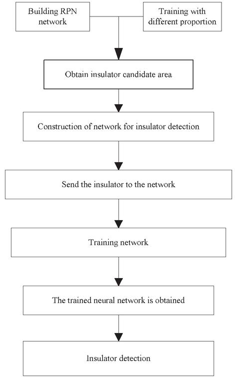
Figure 4 Schematic diagram of network training.

The first step is to train the regional recommendation network, in which the pre trained model on the Image Net dataset is used to initialize the network, and the end-to-end mode is used to fine tune the network;

The second step is to train the Fast R-CNN network by using the region of interest obtained from the candidate region recommendation network as the input of Fast R-CNN. The network is also initialized by using the pre trained model on Image Net. In these two steps, the two are trained separately and there is no convolution feature sharing;

Step 3: the Fast R-CNN network trained in the second step is used to initialize the regional recommendation network, fix all the shared convolution layers, and only fine tune the unique parameter layer of the regional recommendation network. In this way, the mode of volume layer sharing is opened;

Step 4: Similar to step 3, do the same processing, only fine tune the unique full connection layer of Fast R-CNN. After these four steps, the two can share convolution features, and can be unified into a network model to test insulators.

4 Experiment

In the experiment, the insulator data set is constructed by using the existing image data, and the network is trained and tested on the data set. The method of this study is used in the experiment, and the traditional methods are compared to compare the effectiveness of the two methods.

4.1 Experimental Data

Because there is no public power equipment data set, the insulator data set used in this paper is provided by a power research institute. There are 500 images in the data set, each image size is 2048 * 1360, the background is very complex, and contains interference information such as trees, towers, transmission lines and so on. In the experiment, we intercepted 2000 pieces of 500 * 500 image blocks from the image as the training set and test set, each image contains different number of insulators. In order to improve the accuracy of the experimental results, rotation and flipping are used to increase the amount of experimental data to 6000. Use Labelimg software to mark the insulators in the picture. The Figure 5 is an example of the insulators applied in this study.

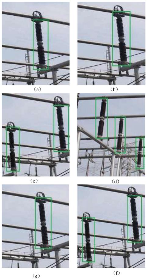
Figure 5 Example diagram of insulator applied in experiment.

4.2 Comparison of Detection Time

The comparison results of the detection time between the detection method of this study and the traditional method are shown in Table 1:

Table 1 Comparison of detection time

Number	The Detection Time of This	Detection Time of
Experiments	Research Method/Min	Traditional Methods/Min
1	2	10
2	2	12
3	3	13
4	4	14
5	5	15
6	2	16
7	3	18
8	6	20

According to the analysis of the above table, the detection time of this research method is less than that of traditional methods, which has strong practical significance.

4.3 Comparison of Detection Accuracy

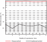
The comparison results of the detection accuracy of the two methods are shown in Figure 6:

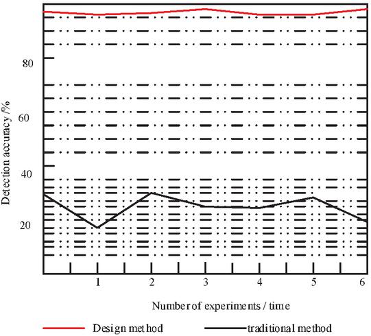
Figure 6 Comparison of detection accuracy.

Through the analysis of the above figure, it is found that the detection accuracy of the research method is much higher than that of the traditional method, which verifies the effectiveness of the research method.

5 Conclusion

This research work is based on the demand of power inspection engineering. Firstly, the basic concept of convolutional neural network, its components, the characteristics and functions of each component are briefly described. Secondly, on the basis of deep theory, the design of each part of convolutional neural network and the construction of the whole network are carried out. Then, aiming at the feature learning ability of training model, the paper combines convolutional neural network and self-organizing mapping network to improve the significance of detection, narrow the search range and accelerate the processing process. The fault detection method of power insulator based on deep convolution neural network is completed. The experimental results show that the method of this study is more accurate than the traditional method.

References

[1] Zhang Y, Lee TS, Li M, et al. Convolutional neural network models of V1 responses to complex patterns[J]. Journal of Computational Neuroscience, 2019, 46(1):33–54.

[2] Li W, Zhang X, Peng Y, et al. Spatiotemporal Fusion of Remote Sensing Images using a Convolutional Neural Network with Attention and Multiscale Mechanisms[J]. International Journal of Remote Sensing, 2021, 42(6):1973–1993.

[3] Xu Y, Li D, Wang Z, et al. A deep learning method based on convolutional neural network for automatic modulation classification of wireless signals[J]. Wireless Networks, 2019, 25(7):3735–3746.

[4] Thirusangu N, Subramanian T, Almekkawy M. Segmentation of induced substantia nigra from transcranial ultrasound images using deep convolutional neural network[J]. The Journal of the Acoustical Society of America, 2020, 148(4):2636–2637.

[5] Nogay HS, Adeli H. Detection of Epileptic Seizure Using Pretrained Deep Convolutional Neural Network and Transfer Learning[J]. European Neurology, 2020, 83(6):602–614.

[6] Ibrahim M, Sagers JD, Ballard MS. A convolutional neural network applied to Arctic acoustic recordings to identify soundscape components[J]. The Journal of the Acoustical Society of America, 2020, 148(4):2687–2687.

[7] Korvel G, Treigys P, Kostek B. Highlighting interlanguage phoneme differences based on similarity matrices and convolutional neural network[J]. The Journal of the Acoustical Society of America, 2021, 149(1):508–523.

[8] Wu H, Wei X, Zha Y, et al. Acoustic spatial patterns recognition based on convolutional neural network and acoustic visualization[J]. The Journal of the Acoustical Society of America, 2020, 147(1):459–468.

[9] Yamane S, Matsuo K. Adaptive Control by Convolutional Neural Network in Plasma Arc Welding System[J]. ISIJ International, 2020, 60(5):998–1005.

[10] Gamdha D, Unnikrishnakurup S, Rose KJJ, et al. Automated Defect Recognition on X-ray Radiographs of Solid Propellant Using Deep Learning Based on Convolutional Neural Networks[J]. Journal of Nondestructive Evaluation, 2021, 40(1):1–13.

[11] Kowal M, Ejmo M, Skobel M, et al. Cell Nuclei Segmentation in Cytological Images Using Convolutional Neural Network and Seeded Watershed Algorithm[J]. Journal of Digital Imaging, 2020, 33(1):231–242.

[12] Shaban M, Awan R, Fraz MM, et al. Context-Aware Convolutional Neural Network for Grading of Colorectal Cancer Histology Images[J]. IEEE Transactions on Medical Imaging, 2020, 39(7):2395–2405.

[13] Allken V, Handegard NO, Rosen S, et al. Fish species identification using a convolutional neural network trained on synthetic data[J]. ICES Journal of Marine Science, 2019, 76(1):342–349.

[14] Xing Y, Xu J, Tan J, et al. Deep convolutional neural network for removal of salt and pepper noise[J]. IET Image Processing, 2019, 13(9):1550–1560.

[15] Sun J, Slang S, Elboth T, et al. A convolutional neural network approach to deblending seismic data[J]. Geophysics, 2019, 85(4):1–57.

[16] Tavakolian M, Hadid A. A Spatiotemporal Convolutional Neural Network for Automatic Pain Intensity Estimation from Facial Dynamics[J]. International Journal of Computer Vision, 2019, 127(10):1–13.

[17] High-Precision Symmetric Weight Update of Memristor by Gate Voltage Ramping Method for Convolutional Neural Network Accelerator[J]. IEEE Electron Device Letters, 2020, 41(3):353–356.

[18] Convolutional neural network-based segmentation can help in assessing the substantia nigra in neuromelaninMRI[J]. Neuroradiology, 2019, 61(12):1387–1395.

[19] Zhang Y, Lee TS, Li M, et al. Convolutional neural network models of V1 responses to complex patterns[J]. Journal of Computational Neuroscience, 2019, 46(1):33–54.

[20] Zhang H, Tong G, Xiong N. Fine-grained CSI fingerprinting for indoor localisation using convolutional neural network[J]. IET Communications, 2020, 14(18):3266–3275.

[21] Hamouda M, Ettabaa KS, Bouhlel MS. Smart Feature Extraction and Classification of Hyperspectral Images based on Convolutional Neural Networks[J]. IET Image Processing, 2020, 14(10):1999–2005.

[22] Neilsen TB, Escobar C, Acree MC, et al. Effect of environmental uncertainty on source localization from mid-frequency tonals using convolutional neural networks[J]. The Journal of the Acoustical Society of America, 2020, 148(4):2544–2544.

[23] Williams D, Espaa A. Toward explainable convolutional neural network classifiers with acoustic-color sonar data[J]. The Journal of the Acoustical Society of America, 2020, 148(4):2661–2661.

[24] Wei R, Song Y, Zhang Y. Enhanced Faster Region Convolutional Neural Networks for Steel Surface Defect Detection[J]. ISIJ international, 2020, 60(3):539–545.

[25] Yu J, Schumann AW, Sharpe SM, et al. Detection of grassy weeds in bermudagrass with deep convolutional neural networks[J]. Weed Science, 2020, 68(5):1–31.

Biographies

Yan Wang was born in 1970 and received her PhD from Tianjin University in China,She has been teaching at Liaoning Technical University in China for more than 20 years. She is an experienced teacher and a forward-looking professor.Her research interests are signal detection and processing.

Weijie Zhang was Born in 1996, he received his bachelor’s degree from Liaoning Technical University in China in 2018 and is currently studying for a master’s degree. His research interests are object recognition and deep learning.

Distributed Generation & Alternative Energy Journal, Vol. 36_2, 97–112.
doi: 10.13052/dgaej2156-3306.3621
© 2021 River Publishers