Metaheuristic Technique based on Realistic Mimicking of Grey Wolf’s Hunting Process for Solving Dynamic Economic Dispatch Problem with Electric Vehicles
Anjali Jain1,*, Ashish Mani1 and Anwar Shahzad Siddiqui2
1Dept. of Electrical and Electronics Engineering, Amity University Uttar Pradesh, Noida, Uttar Pradesh, India
2Dept. of Electrical and Electronics Engineering, Jamia Milia Islamia, Delhi, India
E-mail: anjalijain.121@gmail.com; amani@amity.edu; assiddiqui@jmi.ac.in
*Corresponding Author
Received 06 December 2021; Accepted 05 February 2022; Publication 22 April 2022
Abstract
This paper proposes a realistic variant of grey wolf optimizer with the dynamic behavior of prey position and hence called as Realistic Grey Wolf Optimizer (RGWO). The proposed method is employed to solve 23 benchmark problems and a well-known complex power system problem of dynamic economic dispatch of power by generating units taking into consideration of electric vehicles with valve point effect, ramp-rate, transmission losses for a time interval of 24 hours. The prey position is modeled dynamic i.e., it is considered to be moving and is not static as considered in an earlier version of GWO with the help of probability distribution function. The probability distribution function which is considered here is Levy Flight, Cauchy, Gamma, Gaussian, and Weibull. Thereafter, the statistical testing is done with the help of the Wilcoxon Rank test and Wilcoxon Signed Rank test to investigate the significance of the different variants of RGWO. The experimental results and statistical testing show that the modification proposed in RGWO significantly improves the performance of GWO and hence the algorithm is utilized to find dynamic economic dispatch along with electric vehicles considering different constraints effectively.
Keywords: Metaheuristic, grey wolf optimizer, dynamic prey, probability distribution function, dynamic economic dispatch, electric vehicles.
Nomenclature
| total generation cost | |
| dispatch time | |
| number of generating units | |
| power generated by th unit in th time interval | |
| generation cost of th unit in th time interval | |
| index for unit | |
| index for time | |
| cost coefficients of the th units | |
| minimum power generation limit of th unit | |
| maximum power generation limit of th unit | |
| valve-point coefficients of the th units | |
| power demand of the system at th interval | |
| transmission losses at that time interval | |
| loss coefficients | |
| load due to electric vehicles connected in the network as per the EPRI profile | |
| randomly chosen time interval | |
| ramp-up rate of the th generating unit | |
| ramp-down rate of the th generating unit | |
| grey wolf’s position vector at time | |
| prey position vector at time | |
| coefficient vector used in GWO algorithm | |
| lies between and are random vectors | |
| vector varying linearly decreasing between 2 and 0 | |
| MaxIter | maximum count of iteration |
1 Introduction
The optimized dispatch of power in an electric power system is one of the very complex and important problems for which researchers are continuously working to provide the best solution. Even after continuous research in the given field, the problem still stands because of the ever-increasing demand for power due to growing infrastructure and inclusion of different components such as renewable energy sources, electric vehicles, etc. Thermal generating units have a major contribution in fulfilling the demand. In a grid network, there are many thermal generating units available. Now the question comes which generating unit should produce how much power so that cost of generation can be minimized. The complexity of the problem increases with the inclusion of the valve-point effect, ramp rate constraints, and transmission losses. This problem is referred to as dynamic economic dispatch (DED).
In the power system, the cost of generation is huge and hence an optimum solution is required so that cost of generation can be minimized. Moreover, the problem is complicated, non-convex, and non-differentiable because of valve point effects and ramp rate constraints.
For the reason that the behavior of the DED problem is non-convex, non-differentiable, and non-linear, they are difficult to solve with deterministic techniques. Hence an alternate mechanism is required to find a solution for such cases. Nowadays, meta-heuristic techniques are considered to be an effective tool for finding a solution for such real-world problems. DED problems are also solved by metaheuristic techniques in the available literature. One such algorithm has been discussed in [1], but the issue is there are a lot of parameters to tune to find the optimum solution and hence a new algorithm is required which can serve the purpose with the tuning of a smaller number of parameters and hence the need of finding new algorithm is on.
The motivation for these metaheuristic algorithms is derived from the behavior of species in nature, the behavior of physical phenomenon, and swarm intelligence [2]. Survival of fittest-based algorithms starts with the defined population and is trying to be fitted in the environment. If it fails to do so it is replaced by a new population and so on. In Bio-inspired algorithms, the parent population undergoes various mechanisms of adaptation to produce children. Some of such bio-inspired algorithms are genetic algorithms [3], biogeography-based optimization [4], differential evolution [5], etc. Some of the physical algorithms and their variants that are inspired by physical processes are simulated annealing [6, 7], gravitational search algorithm [8], artificial electric field algorithm [9], harmony search [10, 11], etc.]. The other form of algorithms is based on the collective intelligence of swarms wherein some of the well-known algorithms in this category are PSO (Particle Swarm Optimization) [12], ABC (Artificial Bee Colony) [13], etc. Various metaheuristic algorithm which has been proposed by various researchers are bee colony [14], krill herd [15], fruit fly [16], random forest [17], firefly [18], bat-inspired [19], human opinion [20], neural network [21], pigeon-based [22], and many more. A detailed review of various meta-heuristic techniques has been provided in [23].
Mirjalili et.al, proposed that GWO is a meta-heuristic technique based on the hunting process of grey wolves [24], and the advantage proposed by this method is that this algorithm can be easily implemented, has only a few control parameters to tune, and is also simple. Because of such features, GWO found wide implementation to solve many engineering problems such as economic dispatch of power [25], optimization of power flow [26], optimization of reactive power dispatch [27]. An improved GWO has been proposed in [28] to solve a different engineering problem. In [28], distance learning-based hunting (DLH) has been used to construct a neighborhood of wolves but still, the prey is considered static as in other GWO variants and hence RGWO is proposed to realistically model the prey position in the hunting process by grey wolves. Similarly, other variants available in literature which are proposed by the authors from time to time such as GWO based on learning-based hunting search [29], extended GWO [30, 31], GWO with mutation operator [32], surrogated assisted GWO [33], modified GWO [2, 34, 35], binary GWO [36, 37], hybridized GWO [38–40] with a different algorithm, etc.
Despite various significant characteristics of GWO, [41] claims that GWO is adding no novel contribution, hence the realistic version which is based on realistic behavior or mimicking of prey position in the hunting process is proposed which will prove that GWO is not a just metaphor but also is an efficient algorithm. It has been done with the help of the dynamic behavior of prey. Not only it is realistic mimicking of grey wolves hunting process but also provides better solutions as showcased with the help of statistical testing in the paper.
In this paper, the proposed changes help in the improvement of the convergence speed and also avoid trapping in local optima. The prey position is considered dynamic in nature which is considered to be static as defined in [24]. By dynamic nature of prey, authors want to state that prey is moving whereas in previously available literature prey is considered to be at one position which is also as per the realistic hunt process of wolves. To model the prey position, random distribution functions such as Levy, Cauchy, Gamma, Gauss, and Weibull probability distribution function has been utilized. After that, the performance of RGWO in which prey position is considered to be dynamic is assessed with the performance of original GWO by using Wilcoxon Rank test and Wilcoxon Signed-Rank test [42]. The RGWO algorithm either outperforms or performs competitively as GWO. The analysis has been done on the CEC2005 benchmark test system [43] for unimodal and multimodal problems. Lastly, RGWO is also utilized to find the solution for the power system problem of dynamic economic dispatch and compared with the results produced by GWO.
This paper has been designed for the following outline: Section 1 is about the introduction. Section 2 talks dynamic economic dispatch problem. Section 3 discusses the proposed algorithm along with the evaluation of prey position with the help of different probability distribution functions. Section 4 discusses numerical experiments and results obtained for 23 benchmark problems of CEC2005 and a real-time power system problem of dynamic economic dispatch for 5 generator test cases. Lastly, the conclusion is summed up in Section 5 and the paper ended with the list of references and appendix.
2 Dynamic Economic Dispatch
Dynamic economic dispatch (DED) is a real-time power system problem and is defined as the ideal dispatch solution with the minimum fuel cost in defined time while satisfying operational constraints such as power demand balance, prohibited operating zone, maximum and minimum limit of power generation, and ramp rate constraints [44].
The problem statement with objective function and constraints [44] are as under:
2.1 Objective Function
The objective of the DED problem is defined as
| (1) |
is defined as
| (2) |
2.2 Constraints
The constraints associated with the dynamic economic dispatch problem which are considered in this analysis are as under:
1. Power demand balance The foremost constraint associated with the dispatch problem is to meet generation equal to demand and losses. Hence the sum of generated power by all the generating units at th the time interval must be equal to demand at that time interval plus losses incurred in the system along with the demand enhanced by considering the inclusion of load demand by electric vehicles. Here EPRI load profile [45] is considered for the analysis.
| (3) |
is calculated using approximated B-coefficient loss formula.
| (4) |
If no losses are considered, (4) may be written as
| (5) |
2. Generator maxima and minima limits The generation by any thermal unit lies between its minima and maxima capacity limits. Therefore,
| (6) |
3. Ramp-rate limits The power generated by the thermal units cannot be changed abruptly and hence ramp rate limits are imposed on the generators between the adjacent time intervals. should satisfy the ramp-rate limit as under,
| (7) | ||
| (8) |
Here , The value range of is defined as
| (9) |
3 Realistic Grey Wolf Optimizer (RGWO)
3.1 Classic GWO
Grey wolf Optimizer is a popular algorithm inspired by the hunting process of Canin lupus wolves or grey wolves. The objective of the algorithm is to reach the prey. Wolves are arranged in a hierarchy based on their position in the pack. The hierarchy is decided by the dominance of the wolves. The wolf which is most dominant is at the top and the wolf which is least dominant is at the bottom in the hierarchy. The wolf at the top is said to be an alpha wolf, the next-level position is given to beta wolves and then delta wolves. At the bottom are placed the omega wolves. According to GWO [24], the hierarchal representation of wolves and their features has been shown in Figure 1.
The features of different wolves in the hierarchy are as under:
1. Alpha wolves: Alpha wolves are responsible for taking all major decisions. They lead and manage the pack and they are the first to approach the prey.
2. Beta wolves: The next category of the wolves is beta wolves. Beta wolves obey alpha wolves. They convey and ensure that the decision by alpha wolves is followed by the rest of the wolves.
3. Delta wolves: Wolves on the third hierarchal level is delta wolves. These wolves are hunters, caretakers as well as sentinels. They contribute to the hunting process; caretaker wolves take care of those wolves who are hurt while hunting wherein sentinels wolves protect the pack from enemies.
4. Omega wolves: The last level belongs to omega wolves. They are the least in priority are permitted to eat the hunt at the end. Apart from this, omega wolves are important as in their absence, the pack may face many internal issues.
Figure 1 Wolves in GWO hierarchy along with their features.
The hunting process by grey wolves includes chasing, encircling, searching, and after that attacking the hunt or prey. The detailed modeling of GWO is defined as under:
1. Leadership hierarchy: The fittest solution achieved in optimizing the problem is assumed to be of the -wolf. Then the second-best is of the -wolf, the third-best is of -wolf and the rest of the solutions are assumed to be of -wolves.
2. Encircling of the hunt: The expression for encircling the prey is
| (10) | |
| (11) | |
| (12) | |
| (13) |
3. Hunting: After encircling the hunt, the -wolf guides the pack to hunt the prey. The and wolves help alpha wolves in hunting sometimes. However, wolves do not have any idea about the location of prey. For modeling of hunting behavior, it is presumed that , , and wolves have a better instinct about the current location of prey. Thus, apart from , , and , rest of the wolves modify their position as per (17).
| (14) | |
| (15) | |
| (16) | |
| (17) |
4. Exploring and attacking the prey: This algorithm states that prey is static at the time of the hunt. and defines the exploration and exploitation space of the wolves. The value of and A are 1 refer to exploitation space else to exploration space.
3.2 Proposed RGWO
3.2.1 Modeling and mathematical formulation
In the classic GWO at the time of hunting, the prey is assumed to be t moving whereas as per the realistic model of the hunting process by grey wolves, the prey will always run away from the wolves to save its life, and hence it is proposed that prey position is dynamic in nature. This phenomenon needs to be mathematically modeled in GWO to get more realistic behavior of the hunting process by Canin lupus wolves and behavior of prey. The inclusion of dynamism added to prey will result in overcoming the problem of stagnation in GWO and hence improved the efficacy of the algorithm.
Here in the RGWO, the main contribution is a dynamic model of prey position with the inclusion of different probability distribution functions and and wolves are following prey.
In the original GWO, it was proposed that there are three phases during hunting which are: tracking, chasing, approaching the prey, encircling, and harassing the prey. On the contrary, GWO has not considered all the steps to model the algorithm whereas the inspiration for modeling is taken from only encircling and attacking the prey. To model encircling the prey, (17) is used while attacking is modeled by decreasing the value of linearly from 2 to 0 in (14–16).
In this proposed algorithm, prey position is followed by alpha and beta wolves which are at the top of the hierarchy and hence update their values as per the position of prey, hence resulting in tracking, chasing, and approaching the prey with every iteration as in (19–20). Other wolves are following and wolves and hence result in pursuing the prey. Moreover, as the value of is decreasing from 2 to 0, resulting in encircling the prey as given in (21). Once the stopping criteria are met or prey position is found, the result is printed as per prey position. This process is called attacking the prey.
Prey position plays an important role in the hunting process by grey wolves. Prey is not considered to be static and hence it is moving in different directions to safeguard its life. Therefore, the prey position has been modeled mathematically with the help of the probability distribution function as in (18). Hence, random distribution is considered here to mathematically model the prey pattern with the help of different probability distribution functions (pdf). These pdfs will help to model randomness in prey position. The prey position will be modeled as
| (18) |
The value of alpha and beta wolves are updated as under
| (19) | ||
| (20) |
Delta wolves are updated as per (16).
The new wolves are determined as per greedy search strategy as under:
3.2.2 Algorithmic Design
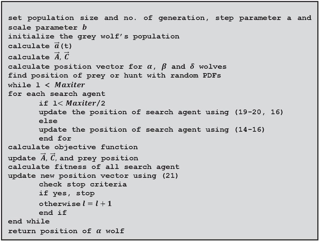
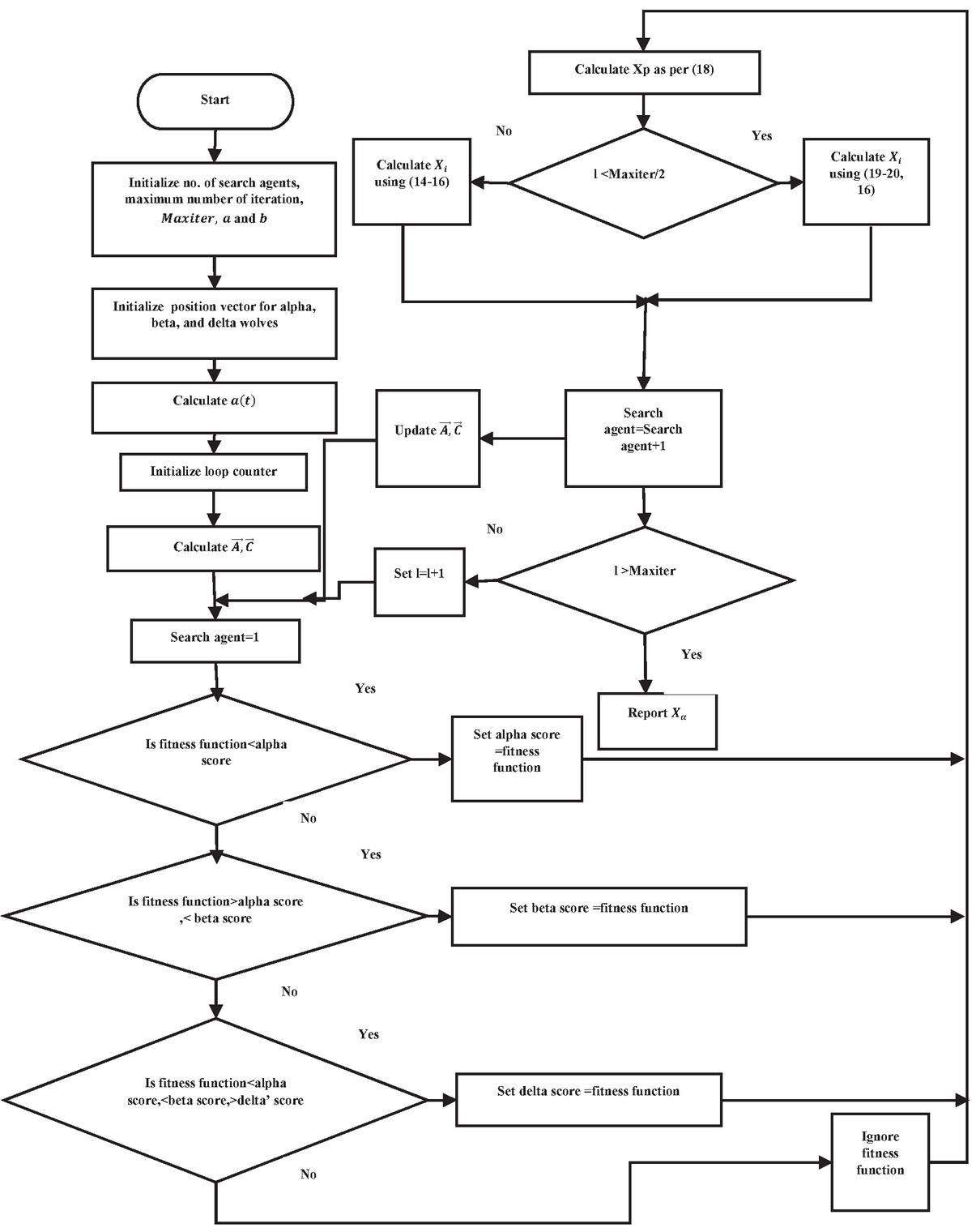
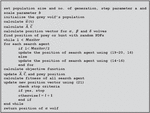
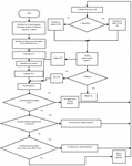
The proper balance between exploration and exploitation is achieved with the value of maximum iteration. For alpha and beta wolves are found as per (19–20), otherwise using (14–15). Also, updating the value of alpha and beta wolves with the help of prey position will add randomness, and hence local stagnation problems can be avoided in the proposed methodology. The pseudo-code for RGWO is shown in Figure 2 and the flowchart has been showcased in Figure 3.
3.2.3 Probability distribution functions
The different probability distribution function which has been considered for the modeling of prey are discussed in this section. As per the proposed methodology, prey is moving and hence it is not realistic to assume the position of prey static. The random behavior of prey needs to be incorporated to give a realistic mimicking of the hunting process. Hence in this section, various probability distribution function has been tried to find out the best fit for modeling the prey position. Following are the different probability distribution functions employed for modeling prey position.
Figure 2 Pseudocode for RGWO.
Figure 3 Flowchart for RGWO.
Levy flight Distribution
The mathematical modeling for levy flight distribution is discussed in [43]. The term levy flight has been used to model random walks. A random walk may be appropriate to model the animal motions more realistically. The following equations define the levy distribution [34]:
| (22) |
Here, represents a variable, represents an index for stability control.
| (23) |
Here, and represent the shift and scale parameters respectively.
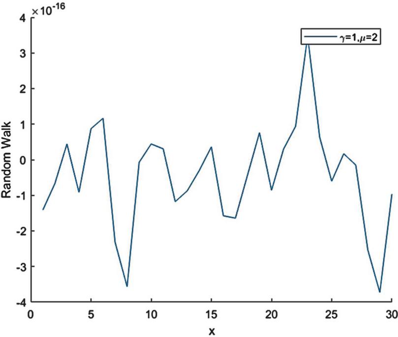
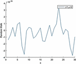
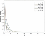
The parameters used for evaluating Levy flight distribution for prey position have been shown in Appendix I. Random walks generated by levy flight distribution for and have been shown in Figure 4.
Figure 4 Random walk by levy distribution for LEVY12.
Cauchy distribution
Cauchy distribution has been used in literature for modeling random walks. It has two parameters x0 and . represents a positive real number and represents the scaling parameter. The equation used to model the Cauchy probability density function is as under [46]:
| (24) |
And for Cauchy cumulative distribution function is
| (25) |
is location parameter and is scale parameter respectively.
The parameters used for evaluating Cauchy distribution for prey position have been shown in Appendix 1.
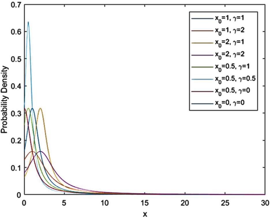
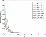
Figure 5 Probability density function for different Cauchy variants.
Gamma distribution
The mathematical modeling for Gamma function is as under [47]:
| (26) |
Here, is the shape parameter and is the scale parameter.
The probability density function is defined as
| (27) |
Also, the gamma function is modeled for all the positive integers.
| (28) |
The cumulative distribution function is:
| (29) |
Here is the lower incomplete Gamma function.
The parameters used for evaluating Gamma distribution for prey position have been shown in Appendix 1.
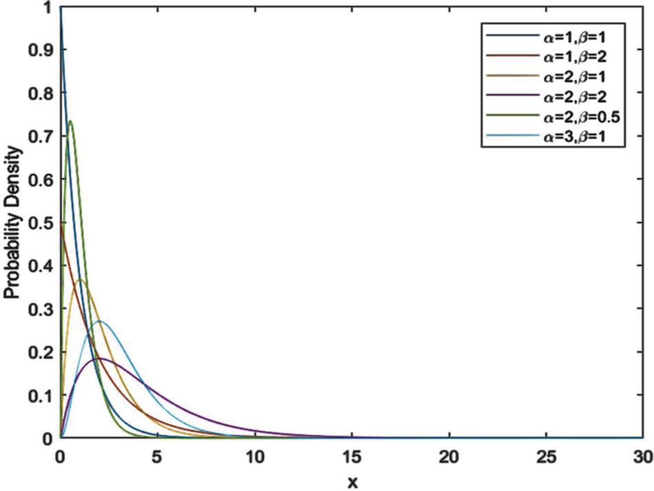
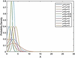
Figure 6 The probability density function for different Gamma variants.
Gaussian distribution
The gaussian distribution also called normal distribution is popularly used for the cases whose distribution is not known. For generating a real-valued random number, Gaussian distribution is frequently employed [48]. Its pdf is defined as
| (30) |
Here is the mean of the distribution and is the standard deviation.
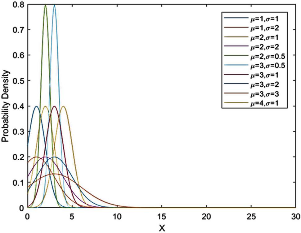
The parameters used for evaluating Gaussian distribution for prey position have been shown in Appendix 1. Figure 7 shows the variation of Gaussian probability density function for different variants as per Appendix 1.
Weibull distribution
Weibull distribution is one of the continuous probability density functions [49]. The pdf of a Weibull random variable is given as
| (31) |
Here’ the scale parameter of Weibull distribution. The parameters used for evaluating Weibull distribution for prey position have been shown in Appendix 1.
Figure 7 The probability density function for different Gauss variants.
4 Experiment for Selection of Parameters
For fixing the parameters utilized in different distribution functions, the proposed algorithm is investigated for 23 benchmark test systems as defined in CEC2005 [43]. The platform used for the evaluation of these experiments is MATLAB R2017b, Windows 10, 5th generation central processing unit @1.60GHz, 8 GB RAM, x64-based processor, and 64-bit operating system. 23 benchmark test functions of CEC2005 are solved with the help of different variants of RGWO including Levy, Cauchy, Gamma, Gaussian, and Weibull probability distribution functions and ranked as per their performance for different benchmark functions.
4.1 Levy Flight Distribution
The best value for 23 benchmark problems obtained by RGWO with prey position modeled as per different variants of Levy distribution for different parameters in Appendix 1 is shown in Appendix 2.
For tuning of Levy distribution parameters, values of and are varied. Appendix 2 shows the best values obtained by benchmark problems with parameters varying from and 2, to 3. When is varying from 1 to 2 the overall rank is reduced from 3 to 1 and hence is utilized. On the other hand, when is varying from 1 to 3, the rank of best value is decreased when moving from 1 to 2 and increased when moving from 2 to 3. Hence it can be concluded that Levy distribution for and is giving a better solution for most of the benchmark problems as compared to its other variants.
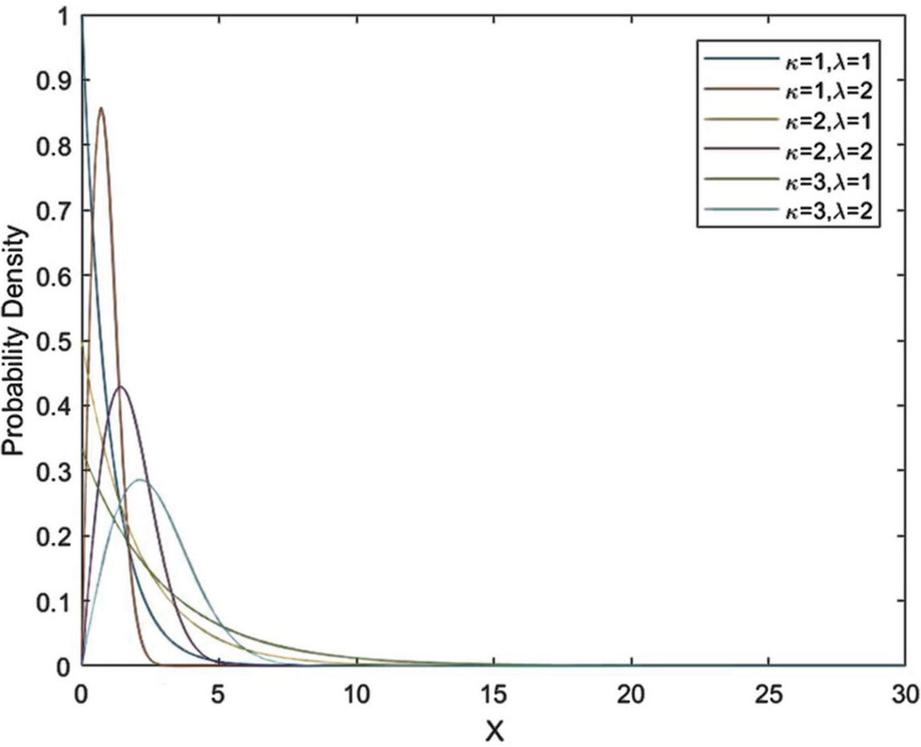
Figure 8 The probability density function for different Weibull variants.
The rank shown in Appendix 2 for different variants of Levy distribution evaluated that if the prey position is modeled as per LEVY12, it is producing better results for most of the benchmark problems amongst all the Levy variants. Hence, in further analysis LEVY12 variant is utilized for modeling of prey position.
4.2 Cauchy Distribution
The best value for 23 benchmark problems obtained by RGWO with prey position modeled as per different variants of Cauchy distribution for different parameters in Appendix 1 is shown in Appendix 3. Figure 5 shows the probability density function for different Cauchy variants with change in and values as per Appendix 1.
Initially for tuning of parameters for Cauchy probability density function, the combination for and are checked but it is found that when and are increasing the rank is also increasing. Hence Cauchy parameters are checked for a combination of and values for 0.5 and 0. It has been found that when and values are further reduced from 1 to 0.5, the rank given for best value has been decreased. Hence it can be concluded that when values are reducing for and values, the better solution is obtained for benchmark problems. On the contrary, if the values are further reduced to 0, the rank is increased which indicates that and values 0.5 used for Cauchy pdf gives a better solution for most of the benchmark problems as compared to other variants of Cauchy distribution.
The rank has been allotted for different variants of Cauchy distribution and it has been evaluated that if the prey position is modeled as per the CAUCHY0.50.5 variant, it is producing better results for most of the benchmark problems amongst all the Cauchy variants a. Hence in further analysis CAUCHY0.50.5 variant is utilized for modeling of prey position.
4.3 Gamma Distribution
The best value for 23 benchmark problems obtained by RGWO with prey position modeled as per different variants of Gamma distribution for different parameters in Appendix 1 is shown in Appendix 4. Figure 6 shows the variation of gamma probability density function for different variants as per Appendix 1.
Initially, for tuning of parameters for Gamma probability density function, the combination for and are checked but it is found that when is increasing from 1 to 2 the rank is decreased but when is increased from 1 to 2, rank is increased. So, to further found the value of the optimum parameter of is further increased but that is not decreasing the rank. hence is fixed to 2 and for finding the better value for , is decreased to 0.5 but that is not giving a better solution for most of the benchmark problems. Hence and is used as a parameter for the gamma probability density function for solving most of the benchmark problems.
The rank has been allotted for different variants of Gamma distribution and it has been evaluated that if the prey position is modeled as per GAMMA21, it is producing better results for most of the benchmark problems amongst all the Gamma variants. Hence in further analysis GAMMA21 variant is utilized for modeling of prey position.
4.4 Gaussian Distribution
The best value for 23 benchmark problems obtained by RGWO with prey position modeled as per different variants of Gaussian distribution for different parameters in Appendix 1 is shown in Appendix 5.
For tuning the parameters for Gaussian distribution, and are varied with a combination of 1 and 2 initially. It was found that when is varying from 1 to 2, the rank is decreased on the contrary when is increased from 1 to 2, the value of rank is increased and it has been noticed that when is decreasing rank is decreasing hence is further iterated for 3 and 4 and it has been observed that gamma probability distribution function is giving better result with and for most of the benchmark problems wherein it has been also noticed that if is further reduced from 1, the values obtained by different benchmark problems are not superior in most of the cases.
The rank has been allotted for different variants of Gaussian distribution and it has been evaluated that if the prey position is modeled as per GAUSS31, it is producing better results for most of the benchmark problems amongst all the Gaussian variants. Hence, in further analysis GAUSS31 variant is utilized for modeling of prey position.
4.5 Weibull Distribution
The best value for 23 benchmark problems obtained by RGWO with prey position modeled as per different variants of Weibull distribution for different parameters in Appendix 1 is shown in Appendix 6. Figure 8 shows the variation of Weibull probability density function for different variants as per Appendix 1.
Initially, for tuning of parameters for the Weibull probability distribution function, the combination for and are checked but it is found that when and are increasing the rank is also increasing. Hence Weibull parameters are also checked for a combination of and . But it has been observed that superior results are obtained for most of the benchmark problems with and .
The rank has been allotted for different variants of Weibull distribution and it has been evaluated that if the prey position is modeled as per WEIBULL22, it is producing better results for most of the benchmark problems amongst all the Weibull variants, and hence in further analysis WEIBULL22 variant is utilized for modeling of prey position.
Table 1 Description of unimodal benchmark problems with the performance of GWO [24] and other variant of RGWO
| Fun | Formulation | D | Calculation | GWO | RGWOLevy | RGWOCauchy | RGWOGamma | RGWOGauss | RGWOWeibull |
| F1 | 30 | Average | 5.712*10-28 | 5.846*10-32 | 2.386*10-16 | 8.386*10-32 | 8.796*10-09 | 4.225*10-32 | |
| St. Dev. | 7.989*10-28 | 1.480*10-31 | 1.109*10-16 | 4.017*10-32 | 4.488*10-09 | 1.111*10-31 | |||
| Best (Min) | 2.210*10-29 | 1.268*10-34 | 8.987*10-17 | 3.354*10-32 | 3.080*10-09 | 2.445*10-34 | |||
| F2 | 30 | Average | 8.490*10-17 | 5.331*10-20 | 2.853*10-08 | 4.807*10-16 | 1.596*10-04 | 6.072*10-20 | |
| St. Dev. | 8.509*10-17 | 5.275*10-20 | 9.323*10-09 | 1.254*10-16 | 5.348*10-05 | 6.670*10-20 | |||
| Best (Min) | 1.240*10-17 | 1.690*10-20 | 1.291*10-08 | 2.440*10-16 | 7.500*10-05 | 2.200*10-21 | |||
| F3 | 30 | Average | 2.307*10-05 | 4.843*10-05 | 6.602*10-06 | 2.370*10-05 | 7.809*10-03 | 3.418*10-05 | |
| St. Dev. | 9.217*10-05 | 1.568*10-04 | 1.497*10-05 | 1.102*10-04 | 8.198*10-03 | 1.632*10-04 | |||
| Best (Min) | 1.770*10-09 | 4.394*10-11 | 1.748*10-10 | 6.325*10-10 | 1.320*10-03 | 6.450*10-10 | |||
| F4 | 30 | Average | 7.111*10-07 | 1.274*10-07 | 1.594*10-06 | 7.556*10-08 | 8.958*10-03 | 1.208*10-07 | |
| St. Dev. | 1.164*10-06 | 2.139*10-07 | 5.777*10-07 | 6.603*10-08 | 3.138*10-03 | 1.890*10-07 | |||
| Best (Min) | 7.566*10-08 | 4.680*10-09 | 8.231*10-07 | 7.990*10-09 | 4.540*10-03 | 4.550*10-09 | |||
| F5 | 30 | Average | 2.696*10+01 | 2.719*10+01 | 2.693*10+01 | 2.695*10+01 | 2.817*10+01 | 2.691*10+01 | |
| St. Dev. | 6.759*10-01 | 6.028*10-01 | 6.868*10-01 | 8.905*10-01 | 1.010*10+00 | 7.529*10-01 | |||
| Best (Min) | 2.610*10+01 | 2.620*10+01 | 2.579*10+01 | 2.520*10+01 | 2.590*10+01 | 2.610*10+01 | |||
| F6 | 30 | Average | 6.997*10-01 | 8.195*10-01 | 8.109*10-01 | 9.455*10-01 | 1.369*10-01 | 7.576*10-01 | |
| St. Dev. | 2.994*10-01 | 3.967*10-01 | 4.709*10-01 | 4.171*10-01 | 1.615*10-01 | 4.255*10-01 | |||
| Best (Min) | 6.520*10-05 | 2.500*10-01 | 5.960*10-05 | 2.501*10-01 | 5.193*10-05 | 7.300*10-05 | |||
| F7 | 30 | Average | 1.749*10-03 | 1.666*10-03 | 1.560*10-03 | 1.770*10-03 | 2.139*10-02 | 1.223*10-03 | |
| St. Dev. | 8.517*10-04 | 9.517*10-04 | 1.200*10-03 | 1.128*10-03 | 7.446*10-03 | 6.028*10-04 | |||
| Best (Min) | 4.230*10-04 | 1.077*10-04 | 3.393*10-04 | 2.789*10-04 | 9.190*10-03 | 1.740*10-04 |
Table 2 Description of multimodal, high dimension benchmark problems with the performance of GWO [24] and other variant of RGWO
| Fun | Formulation | D | Calculation | GWO | RGWOLevy | RGWOCauchy | RGWOGamma | RGWOGauss | RGWOWeibull |
| F8 | ) | 30 | Average | -6.117*10+03 | 5.794*10+03 | 6.064*10+03 | 5.800*10+03 | 5.616*10+03 | 6.032*10+03 |
| St. Dev. | 6.656*10+02 | 6.989*10+02 | 7.991*10+02 | 7.402*10+02 | 6.583*10+02 | 7.885*10+02 | |||
| Best (Min) | -7.860*10+03 | 7.755*10+03 | 7.355*10+03 | 7.360*10+03 | 6.720*10+03 | 7.350*10+03 | |||
| F9 | 30 | Average | 3.113*10+00 | 1.201*10-01 | 3.975*10-01 | 4.197*10-01 | 5.111*10+01 | 6.670*10-01 | |
| St. Dev. | 3.902*10+00 | 6.578*10-01 | 1.524*10+00 | 1.778*10+00 | 3.263*10+01 | 1.675*10+00 | |||
| Best (Min) | 0.000*10+00 | 0.000*10+00 | 5.684*10-13 | 0.000*10+00 | 2.720*10+01 | 0.000*10+00 | |||
| F10 | 30 | Average | 9.859*10-14 | 3.395*10-14 | 1.167*10-08 | 4.293*10-14 | 6.610*10-05 | 3.453*10-14 | |
| St. Dev. | 1.377*10-14 | 5.767*10-15 | 3.173*10-09 | 6.452*10-15 | 2.288*10-05 | 7.387*10-15 | |||
| Best (Min) | 7.550*10-14 | 2.220*10-14 | 6.621*10-09 | 2.220*10-14 | 3.180*10-05 | 2.220*10-14 | |||
| F11 | 30 | Average | 4.050*10-03 | 2.227*10-03 | 3.244*10-03 | 8.151*10-04 | 7.250*10-03 | 1.045*10-03 | |
| St. Dev. | 8.575*10-03 | 5.919*10-03 | 1.108*10-02 | 3.105*10-03 | 1.195*10-02 | 4.281*10-03 | |||
| Best (Min) | 0.000*10+00 | 0.000*10+00 | 0.000*10+00 | 0.000*10+00 | 2.210*10-10 | 0.000*10+00 | |||
| F12 | 30 | Average | 1.665*10-03 | 9.380*10-02 | 5.549*10-02 | 6.236*10-02 | 6.055*10-04 | 8.165*10-02 | |
| St. Dev. | 9.516*10-04 | 1.305*10-01 | 2.532*10-02 | 3.096*10-02 | 1.819*10-03 | 9.698*10-02 | |||
| Best (Min) | 1.080*10-04 | 1.230*10-02 | 2.722*10-02 | 2.350*10-02 | 6.890*10-06 | 2.510*10-02 | |||
| F13 | 30 | Average | 5.772*10-01 | 8.148*10-01 | 7.983*10-01 | 7.031*10-01 | 5.528*10-02 | 7.551*10-01 | |
| St. Dev. | 1.915*10-01 | 2.509*10-01 | 2.430*10-01 | 2.258*10-01 | 7.091*10-02 | 2.156*10-01 | |||
| Best (Min) | 1.920*10-01 | 2.980*10-01 | 2.015*10-01 | 3.120*10-01 | 7.360*10-05 | 2.140*10-01 | |||
Table 3 Description of multimodal, low dimension benchmark problem with performance of GWO [24] and other variant of RGWO
| Fun | Formulation | D | Calculation | GWO | RGWOLevy | RGWOCauchy | RGWOGamma | RGWOGauss | RGWOWeibull |
| F14 | 2 | Average | 3.846*10+00 | 4.076*10+00 | 4.719*10+00 | 5.141*10+00 | 3.944*10+00 | 5.383*10+00 | |
| St. Dev. | 3.795*10+00 | 3.864*10+00 | 4.256*10+00 | 4.406*10+00 | 3.934*10+00 | 4.253*10+00 | |||
| Best (Min) | 9.980*10-01 | 9.980*10-01 | 9.980*10-01 | 9.980*10-01 | 9.980*10-01 | 9.980*10-01 | |||
| F15 | 4 | Average | 4.432*10-03 | 1.152*10-03 | 5.797*10-03 | 2.524*10-03 | 4.481*10-03 | 3.139*10-03 | |
| St. Dev. | 8.124*10-03 | 3.645*10-03 | 8.938*10-03 | 6.069*10-03 | 8.097*10-03 | 6.877*10-03 | |||
| Best (Min) | 3.080*10-04 | 3.070*10-04 | 3.075*10-04 | 3.080*10-04 | 3.130*10-04 | 3.075*10-04 | |||
| F16 | 2 | Average | 1.030*10+00 | 1.032*10+00 | -1.032*10+00 | 1.032*10+00 | 1.030*10+00 | 1.032*10+00 | |
| St. Dev. | 4.517*10-16 | 2.537*10-08 | 4.498*10-08 | 2.537*10-08 | 4.517*10-16 | 3.051*10-08 | |||
| Best (Min) | 1.030*10+00 | -1.032*10+00 | -1.032*10+00 | -1.032*10+00 | 1.030*10+00 | -1.032*10+00 | |||
| F17 | 2 | Average | 3.980*10-01 | 3.979*10-01 | 3.979*10-01 | 3.979*10-01 | 3.980*10-01 | 3.979*10-01 | |
| St. Dev. | 1.694*10-16 | 2.308*10-06 | 3.222*10-06 | 4.897*10-06 | 1.694*10-16 | 3.022*10-06 | |||
| Best (Min) | 3.980*10-01 | 3.979*10-01 | 3.979*10-01 | 3.979*10-01 | 3.980*10-01 | 3.979*10-01 | |||
| F18 | 2 | Average | 3.000*10+00 | 3.000*10+00 | 3.000*10+00 | 3.000*10+00 | 3.000*10+00 | 3.000*10+00 | |
| St. Dev. | 6.128*10-05 | 0.000*10+00 | 7.659*10-05 | 0.000*10+00 | 0.000*10+00 | 0.000*10+00 | |||
| Best (Min) | 3.000*10+00 | 3.000*10+00 | 3.000*10+00 | 3.000*10+00 | 3.000*10+00 | 3.000*10+00 | |||
| F19 | 3 | Average | 3.861*10+00 | 3.861*10+00 | -3.862*10+00 | 3.860*10+00 | 3.857*10+00 | 3.860*10+00 | |
| St. Dev. | 2.557*10-03 | 2.916*10-03 | 2.292*10-03 | 1.826*10-03 | 4.795*10-03 | 0.000*10+00 | |||
| Best (Min) | 3.863*10+00 | -3.863*10+00 | 3.863*10+00 | 3.860*10+00 | 3.860*10+00 | 3.860*10+00 | |||
| F20 | 6 | Average | -3.264*10+00 | 3.235*10+00 | 3.277*10+00 | 3.244*10+00 | 3.167*10+00 | 3.213*10+00 | |
| St. Dev. | 7.393*10-02 | 8.279*10-02 | 6.794*10-02 | 6.616*10-02 | 3.095*10-02 | 9.563*10-02 | |||
| Best (Min) | 3.320*10+00 | 3.320*10+00 | -3.322*10+00 | 3.320*10+00 | 3.200*10+00 | 3.322*10+00 | |||
| F21 | 4 | Average | -1.040*10+01 | 9.870*10+00 | 8.311*10+00 | 9.438*10+00 | 1.022*10+01 | 1.005*10+01 | |
| St. Dev. | 1.807*10-15 | 1.616\*10+00 | 2.938*10+00 | 2.222*10+00 | 9.701*10-01 | 1.343*10+00 | |||
| Best (Min) | 1.040*10+01 | 1.040*10+01 | 1.015*10+01 | 1.040*10+01 | 1.040*10+01 | -1.040*10+01 | |||
| F22 | 4 | Average | -1.040*10+01 | 9.870*10+00 | 1.005*10+01 | 9.438*10+00 | 1.022*10+01 | 1.005*10+01 | |
| St. Dev. | 1.807*10-15 | 1.616*10+00 | 1.348*10+00 | 2.222*10+00 | 9.701*10-01 | 1.343*10+00 | |||
| Best (Min) | 1.040*10+01 | 1.040*10+01 | -1.040*10+01 | 1.040*10+01 | 1.040*10+01 | 1.040*10+01 | |||
| F23 | 4 | Average | 1.036*10+01 | 9.724*10+00 | 1.008*10+01 | 9.603*10+00 | -1.050*10+01 | 1.005*10+01 | |
| St. Dev. | 9.787*10-01 | 2.148*10+00 | 1.751*10+00 | 2.379*10+00 | 0.000*10+00 | 1.743*10+00 | |||
| Best (Min) | -1.054*10+01 | 1.054*10+01 | 1.054*10+01 | 1.050*10+01 | 1.050*10+01 | 1.050*10+01 |
5 Performance Analysis of RGWO Variants on Different Benchmark
The variants finalized for comparison are LEVY12, CAUCHY0.50.5, GAMMA21, GAUSS31, WEIBULL22 as discussed in the above section. The performance of different variants is on unimodal and multimodal high dimension and low dimension problems. Therefore, the different variants of Levy, Cauchy, Gamma, Gaussian, and Weibull pdf are compared with GWO, and results for average, standard deviation, and best value for different test cases have been reported in the following subsection.
As per the conclusion drawn for prey modeling using different variants in the previous section, it has been found that LEVY12, CAUCHY0.50.5, GAMMA21, GAUSS31, and WEIBULL22 are providing the best values in their categories.
The performance of the said variants by different PDFs are now compared with GWO to conclude which amongst them may be treated as best for prey modeling. Hence RGWO with different pdf’s are run 30 times and average, standard deviation, and best (minimum) values for different benchmark problems are reported in Tables 1–3.
5.1 Exploitation analysis
In CEC 2005 benchmark test function, the first seven functions are unimodal functions (F1–F7) which are having just one global best. The evaluation of these functions is checked for GWO and different versions of RGWO. The average, standard deviation, and minimum best obtained by these algorithms are given in Table 7.
Table 1 depicts that the RGWO variant with Levy, Gamma, and Weibull pdfs are giving better minimum best values for F1 to F7 except for F6 whereas the Cauchy variant and Gauss variant give the better minimum best value for F6. Also, problems having narrow valley from local optimum to global optimum are solved in a better way by Gaussian and Cauchy distribution function as in F6 Thus it can be easily concluded that making prey position dynamic improves the exploitation capability as well.
The realistic version of GWO works well for the unimodal, shifted, non-separable and scalable problems, Levy, Gamma, and Weibull distribution are giving superior results as demonstrated for all functions except F6 wherein for F6 superior results for best minimum values are obtained by Cauchy and Gauss variants when the problem properties are rotated.
Moreover, from Table 1, it can be concluded that a realistic version of GWO with dynamic prey is giving better values as compared to GWO
This has been further tested by the Wilcoxon rank and Wilcoxon signed-rank test [42] in the coming section.
5.2 Exploration Analysis
In CEC 2005 benchmark functions [43], seventeen functions i.e., F8–F23 are classified as multimodal test cases which are having multiple local optima. These functions help judge the exploratory capabilities of the algorithm. The results obtained by GWO and different variants of RGWO have been reported in Table 2 for multimodal high dimension problems and in Table 3 for multimodal low dimension problems.
Based on results obtained by GWO and RGWO, it is clear that RGWO and its variants are giving either better or competitive values in comparison with GWO for F8–F23 except for F8, F12–13, F22–23 whereas for F8, F12–13, F22–23 Cauchy and Gauss distribution functions are giving superior results as shown in Tables 1–3. The capability for the different algorithms will be tested using statistical testing in the next section.
From Tables 1–3, it is concluded that Levy, Gamma, and Weibull distribution are best suited for prey position modeling and hence comparative convergence curve and statistical testing will be done between GWO and RGWO with Levy, Gamma and Weibull pdfs.
5.3 Convergence analysis
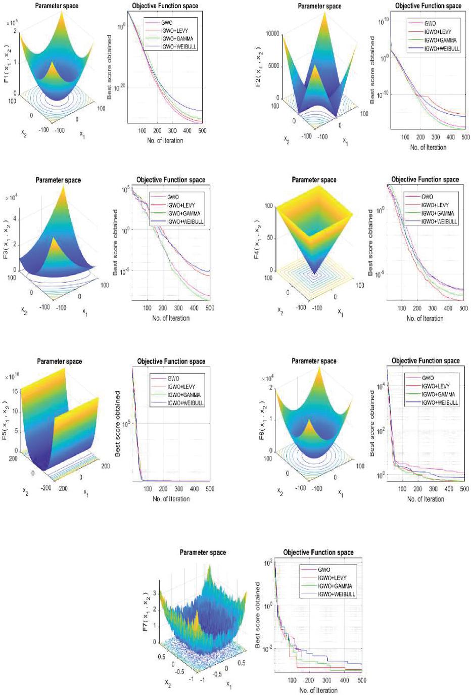
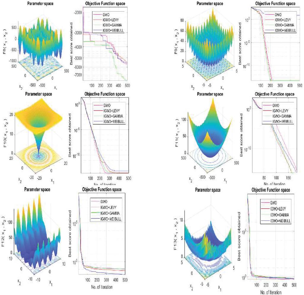
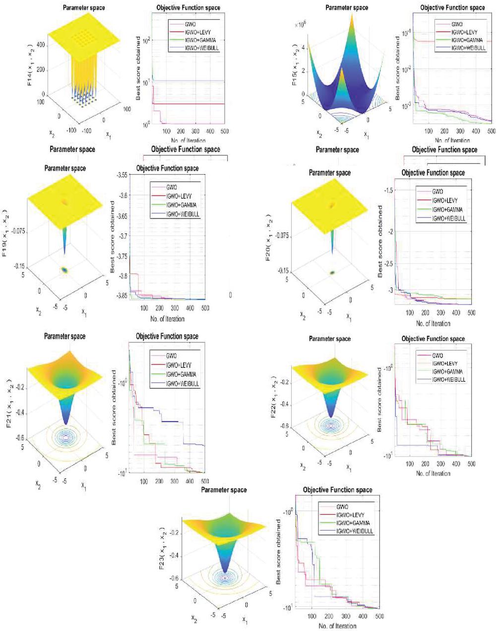
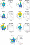
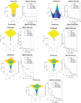
Convergence curves and 3D maps obtained from GWO and RGWO with different distribution for functions F1–F7 are shown in Figure 9, for F8–F13 are shown in Figure 10 and for F14–F23 are shown in Figure 11.
From the above analysis, it is found that RGWO with the modified prey position with the different probability distribution function qualifies that RGWO either outperforms or gives competitive results in comparison to GWO. From the convergence curves shown in Figures 9–11, it can be easily seen that adding a random jump to the prey position leads to faster convergence, and also the global search tendency of the algorithm is improved. Adding random jumps to wolves’ position by modifying the prey position helps the population in preventing the diversity loss and hence improves global search and prevents it from being stuck in local optima.
5.4 Statistical Testing by Wilcoxon Test
Hypothesis testing is employed to draw inferences about one or more populations from given samples or results. For this, two hypotheses are defined that are H0 (null hypothesis) and H1 (alternative hypothesis) [42]. The null hypothesis is a statement of no effect or no difference, whereas the alternative hypothesis represents the presence of an effect or a difference (in our case, significant differences between algorithms). When applying a statistical procedure to reject a hypothesis, a level of significance is used to determine at which level the hypothesis may be rejected. In this study, is chosen as 0.05, the total number of independent runs is 30, the average and their standard deviations have been calculated as shown in Tables 8–9. As per [42], Wilcoxon’s signed-rank test is used to perform the comparison of GWO with different variants of RGWO.
Wilcoxon signed ranked test [42] is used to validate the results statistically. H0 and H1 represent the null and alternate hypotheses for each test case. The null hypothesis states that there is no difference between GWO and RGWO whereas the alternate hypothesis states that there is a difference between the two algorithms and RGWO performs better. R() states the rank at which the alternate hypothesis won and R() states the rank for which the null hypothesis won.
Figure 9 Parameter space graphs and Best score vs Number of iteration curve of the GWO and another variant of RGWO for F1-F7 test cases.
Figure 10 Parameter space graphs and Best score vs Number of iteration curve of the GWO and RGWO and another variant of RGWO for F8-F13 test cases.
Figure 11 Parameter space graphs and best score vs Number of iteration curve of the GWO and RGWO and another variant of RGWO for F17–F23 test cases.
Table 4 Statistical results by Wilcoxon signed rank test comparing RGWO with GWO
| Comparison | Function | Rank() | Rank() | N | p-value |
| RGWOLevy vs GWO | F1 | 465 | 0 | 30 | 0 |
| RGWOGamma vs GWO | F1 | 465 | 0 | 30 | 0 |
| RGWOWeibull vs GWO | F1 | 465 | 0 | 30 | 0 |
| RGWOLevy vs GWO | F2 | 465 | 0 | 30 | 0 |
| RGWOWeibull vs GWO | F2 | 465 | 0 | 30 | 0 |
| RGWOLevy vs GWO | F3 | 335 | 130 | 30 | 0.0175 |
| RGWOLevy vs GWO | F4 | 433 | 32 | 30 | 0 |
| RGWOGamma vs GWO | F4 | 457 | 8 | 30 | 0 |
| RGWOWeibull vs GWO | F4 | 445 | 20 | 30 | 0 |
| RGWOWeibull vs GWO | F7 | 346 | 119 | 30 | 0.0098 |
| RGWOLevy vs GWO | F9 | 382 | 53 | 29 | 0.0002 |
| RGWOGamma vs GWO | F9 | 385 | 21 | 28 | 0 |
| RGWOWeibull vs GWO | F9 | 334 | 72 | 28 | 0.0014 |
| RGWOLevy vs GWO | F10 | 465 | 0 | 30 | 0 |
| RGWOGamma vs GWO | F10 | 465 | 0 | 30 | 0 |
| RGWOWeibull vs GWO | F10 | 465 | 0 | 30 | 0 |
| RGWOLevy vs GWO | F12 | 465 | 0 | 30 | 0 |
| RGWOGamma vs GWO | F12 | 465 | 0 | 30 | 0 |
| RGWOWeibull vs GWO | F12 | 465 | 0 | 30 | 0 |
| RGWOLevy vs GWO | F16 | 465 | 0 | 30 | 0 |
| RGWOGamma vs GWO | F16 | 465 | 0 | 30 | 0 |
| RGWOWeibull vs GWO | F16 | 465 | 0 | 30 | 0 |
| RGWOLevy vs GWO | F17 | 465 | 0 | 30 | 0 |
| RGWOGamma vs GWO | F17 | 465 | 0 | 30 | 0 |
| RGWOWeibull vs GWO | F17 | 465 | 0 | 30 | 0 |
| RGWOLevy vs GWO | F18 | 465 | 0 | 30 | 0 |
| RGWOGamma vs GWO | F18 | 465 | 0 | 30 | 0 |
| RGWOWeibull vs GWO | F18 | 465 | 0 | 30 | 0 |
| RGWOWeibull vs GWO | F22 | 403 | 62 | 30 | 0.0002 |
Table 5 Statistical results by Wilcoxon test comparing RGWO with different distribution
| Rank | Rank | Rank()– | Detected | ||||
| Comparison | Function | () | () | n | Rank() | n/2sqrt(n) | Difference |
| RGWOGamma vs GWO | F3 | 313 | 152 | 30 | 161 | 20.47722558 | |
| RGWOLevy vs GWO | F7 | 242 | 223 | 30 | 19 | 20.47722558 | |
| RGWOGamma vs GWO | F7 | 253 | 212 | 30 | 41 | 20.47722558 | |
| RGWOLevy vs GWO | F11 | 32 | 13 | 9 | 19 | 7.5 | |
| RGWOGamma vs GWO | F11 | 39 | 6 | 9 | 33 | 7.5 | |
| RGWOWeibull vs GWO | F11 | 42 | 13 | 10 | 29 | 8.16227766 | |
| RGWOLevy vs GWO | F15 | 257 | 178 | 29 | 79 | 19.88516481 | |
| RGWOGamma vs GWO | F15 | 200.5 | 177.5 | 27 | 23 | 18.69615242 | |
| RGWOWeibull vs GWO | F15 | 249 | 216 | 30 | 33 | 20.47722558 | |
| RGWOLevy vs GWO | F19 | 269 | 196 | 30 | 73 | 20.47722558 |
Another test utilized to check the overall performance of the algorithm is the Wilcoxon Rank test [42] wherein if the number of wins is at least , then the algorithm is significantly better with p 0.05
As per the above discussion in this section, GWO is compared with different variants of RGWO such as LEVY12, GAMMA21, WEIBULL22 using Wilcoxon Signed Rank Test and Wilcoxon Rank test. It has been observed that the null hypothesis is rejected by all the variants of RGWO for F1, F4, F9, F10, F12, F16, F17 using the Wilcoxon Signed-Rank test. In addition to that, the null hypothesis is rejected by RGWO with LEVY12 for F2 and F3 whereas rejected for F2, F7, and F22 by RGWO with WEIBULL22 using Wilcoxon Signed Rank Test. The summary where RGWO and its variants won over GWO based on Wilcoxon signed-rank test [42] has been shown in Table 4. It has been clearly shown that when modeling the dynamic behavior of prey with the help of Levy, Gamma, and Weibull distribution function, the performance of the algorithm is improved.
Also, RGWO rejects the null hypothesis for F11 and F15 with all the mentioned variants as per Wilcoxon Rank Test [42]. In addition to that, RGWO with LEVY12 variant rejects null hypothesis for F7 and F19 wherein RGWO with GAMMA 21 Variant rejects null hypothesis for F3 and F7. Wilcoxon signed test [42] has been utilized in Table V to show that RGWO performs better than GWO for F3, F5, F7, F11, F15, and F19 by considering the prey dynamic.
Hence, we can conclude that adding random behavior to prey position with the help of either Levy or Gamma or Weibull pdf enhances the exploration capabilities and will be having competitive exploitation capabilities as well.
6 Deployment of RGWO for Dynamic Economic Dispatch Problem
Based on the conclusion drawn from the analysis of result by benchmark system, RGWO with prey position modeled with the Levy, Gamma, and Weibull distribution function is used to solve a DED of power for 5 generator test case [50].
In this analysis, 30 is the population size 500 is the maximum number of iterations. It is to be noted that all the variants of RGWO and GWO are run for a similar repair method to perform a fair comparison amongst the different algorithms. The outcome obtained using RGWO with prey modeled with different PDFs for DED is shown in Table 12 for 5 generators for 24 hours.
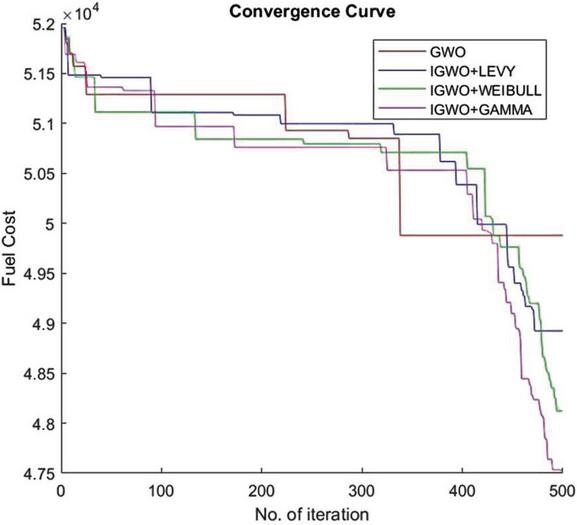
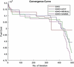
Table 6 also clearly shows that the results provided by RGWO are performing better than GWO. Figure 12 shows the comparison of convergence curve for the said problem with GWO and RGWO where prey position has been modeled with the help of Levy, Gamma, and Weibull distribution.
Figure 12 clearly shows that GWO is stagnant and provides poor results as compared to the variants of RGWO. The variants of RGWO show good exploration at the beginning and good exploitation at the end as suggested by the proposed algorithm.
Figure 12 Comparative Convergence curve for DED 5 Gen Test case with GWO and different variants of RGWO.
Table 6 Comparative performance by GWO and the different variant of RGWO for DED 5 gen test case
| Algorithm | Fuel Cost ($/day) | Decrease in Cost w.r.t GWO |
| GWO | 49879 | |
| RGWOLEVY | 48925 | 1.91% |
| RGWOWEIBULL | 48124 | 3.52% |
| RGWOGAMMA | 47519 | 4.73% |
It has been observed that RGWO with GAMMA21 is giving the best of results amongst all the variants and is showing 4.73% decrease in cost as compared to classic GWO. It is also noted that GWO is stagnating for a long duration and not able to explore hence not able to reach a better solution in the maximum iteration count wherein RGWO variants are showing fast convergence. It is also showcased by the convergence curve that RGWO can be successfully employed for obtaining a better solution for power system problems.
7 Conclusion
The realistic grey wolf optimizer (RGWO) proposed in this paper has been modeled considering the dynamic prey position in place of its static behavior as was considered in the original GWO. Different probability distribution functions have been utilized to showcase the mathematical modeling of prey position. Simulation testing has been done with different probability distribution functions to finalize the step size and scale parameters of different pdfs. It has been observed that the use of probability distribution function to model the prey behavior has improved the performance of the algorithm which has been showcased on 23 benchmark problems. The performance of these methods has been evaluated with the help of the Wilcoxon rank and Wilcoxon signed-rank test. The statistical testing proved that the proposed algorithm is effective for benchmark problems and hence can be applied for complex problems as well. Moreover, the performance of the RGWO is analyzed on the real-time power system problem of dynamic economic dispatch problem for the 5-gen test case and it has been observed that dynamic prey modeling results in improved performance.
Hence it is concluded that RGWO is an efficient metaheuristic to tackle multimodal problems successfully. The future scope of work includes the implementation of the concept proposed in the multi-objective version of RGWO. Towards the end, the authors feel that the work proposed will rouse other researchers to utilize the proposed work for solving various real-time optimization problems.
Appendix
Appendix 1: Parameters of optimizers
| Description of Algorithm | Parameter | Description of Algorithm | Parameter |
| LEVY11 | GAMMA20.5 | ||
| LEVY12 | GAMMA31 | ||
| LEVY21 | GAUSS11 | ||
| LEVY22 | GAUSS12 | ||
| LEVY13 | GAUSS21 | ||
| CAUCHY11 | GAUSS22 | ||
| CAUCHY12 | GAUSS20.5 | ||
| CAUCHY21 | GAUSS30.5 | ||
| CAUCHY22 | GAUSS31 | ||
| CAUCHY0.51 | GAUSS32 | ||
| CAUCHY0.50.5 | GAUSS33 | ||
| CAUCHY0.50 | GAUSS41 | ||
| CAUCHY01 | WEIBULL11 | ||
| CAUCHY00 | WEIBULL12 | ||
| GAMMA11 | WEIBULL21 | ||
| GAMMA12 | WEIBULL22 | ||
| GAMMA21 | WEIBULL32 | ||
| GAMMA22 | WEIBULL33 |
Appendix 2: Best Solution and rank of LEVY Variant for Benchmark function
| Fun | Parameter | LEVY11 | LEVY12 | LEVY21 | LEVY22 | LEVY13 |
| F1 | Best value | 2.3551*10-06 | 7.2244*10-34 | 1.0692*10-05 | 1.7112*10-18 | 6.5861E+04 |
| Rank | 3 | 1 | 4 | 2 | 5 | |
| F2 | Best value | 3.6753*10-03 | 5.4322*10-20 | 1.0444*10-02 | 1.0030*10-10 | 2.4206E+11 |
| Rank | 3 | 1 | 4 | 2 | 5 | |
| F3 | Best value | 1.0844*10+00 | 2.9190*10-07 | 4.8644*10+00 | 1.6319*10+00 | 1.7850E+05 |
| Rank | 2 | 1 | 4 | 3 | 5 | |
| F4 | Best value | 3.6377*10-02 | 2.0111*10-08 | 2.0053*10-01 | 1.5811*10-03 | 9.0908E+01 |
| Rank | 3 | 1 | 4 | 2 | 5 | |
| F5 | Best value | 2.8086*10+01 | 2.7947*10+01 | 2.8623*10+01 | 2.6041*10+01 | 3.1247E+08 |
| Rank | 3 | 2 | 4 | 1 | 5 | |
| F6 | Best value | 1.7933*10+00 | 8.4232*10-01 | 2.0392*10+00 | 6.6007*10-05 | 6.5617E+04 |
| Rank | 3 | 2 | 4 | 1 | 5 | |
| F7 | Best value | 2.2079*10-02 | 2.0124*10-03 | 2.2378*10-02 | 1.1846*10-02 | 1.1279E+02 |
| Rank | 3 | 1 | 4 | 2 | 5 | |
| F8 | Best value | 6.6781*10+03 | 7.1590*10+03 | 7.5686*10+03 | 6.8627*10+03 | 1.5429E+03 |
| Rank | 4 | 2 | 1 | 3 | 5 | |
| F9 | Best value | 4.9698*10+01 | 5.6843*10-14 | 5.9431*10+01 | 4.2908*10+01 | 4.2811E+02 |
| Rank | 3 | 1 | 4 | 2 | 5 | |
| F10 | Best value | 1.0306*10-03 | 4.3521*10-14 | 9.1909*10-04 | 5.2026*10-08 | 2.0366E+01 |
| Rank | 4 | 1 | 3 | 2 | 5 | |
| F11 | Best value | 1.6865*10-07 | 0.0000*10+00 | 2.7109*10-02 | 2.5607*10-02 | 5.4615E+02 |
| Rank | 2 | 1 | 4 | 3 | 5 | |
| F12 | Best value | 1.1971*10-01 | 3.3140*10-02 | 1.7133*10+00 | 1.3206*10-01 | 6.1614E+08 |
| Rank | 2 | 1 | 4 | 3 | 5 | |
| F13 | Best value | 1.1340*10+00 | 8.6441*10-01 | 8.5920*10-01 | 1.0483*10-01 | 1.0529E+09 |
| Rank | 4 | 3 | 2 | 1 | 5 | |
| F14 | Best value | 9.9800*10-01 | 9.9800*10-01 | 9.9800*10-01 | 9.9800*10-01 | 1.5881E+02 |
| Rank | 1 | 1 | 1 | 1 | 5 | |
| F15 | Best value | 4.1355*10-04 | 3.1375*10-04 | 5.4917*10-04 | 3.8958*10-04 | 1.5752E-01 |
| Rank | 3 | 1 | 4 | 2 | 5 | |
| F16 | Best value | 1.0316*10+00 | 1.0316*10+00 | 1.0316*10+00 | 1.0316*10+00 | 1.4543E-01 |
| Rank | 1 | 1 | 1 | 1 | 5 | |
| F17 | Best value | 3.9789*10-01 | 3.9789*10-01 | 3.9789*10-01 | 3.9790*10-01 | 5.1557E+00 |
| Rank | 1 | 1 | 1 | 4 | 5 | |
| F18 | Best value | 3.0000*10+00 | 3.0000*10+00 | 3.0002*10+00 | 3.0000*10+00 | 3.2914E+01 |
| Rank | 1 | 1 | 4 | 1 | 5 | |
| F19 | Best value | 3.8607*10+00 | 3.8618*10+00 | 3.8616*10+00 | 3.8621*10+00 | 3.3605E+00 |
| Rank | 4 | 2 | 3 | 1 | 5 | |
| F20 | Best value | 3.1534*10+00 | 3.3220*10+00 | 3.1335*10+00 | 3.2024*10+00 | 1.6398E+00 |
| Rank | 3 | 1 | 4 | 2 | 5 | |
| F21 | Best value | 1.0151*10+01 | 1.0151*10+01 | 1.0151*10+01 | 1.0153*10+01 | 1.2189E+00 |
| Rank | 2 | 4 | 3 | 1 | 5 | |
| F22 | Best value | 1.0402*10+01 | 1.0400*10+01 | 1.0401*10+01 | 1.0401*10+01 | 5.8508E-01 |
| Rank | 1 | 4 | 3 | 2 | 5 | |
| F23 | Best value | 1.0535*10+01 | 1.0535*10+01 | 1.0535*10+01 | 1.0535*10+01 | 8.7607E-01 |
| Rank | 4 | 1 | 3 | 1 | 5 | |
| OVERALL RANK | 3 | 1 | 4 | 2 | 5 | |
Appendix 3: Best Solution and rank of CAUCHY Variant for Benchmark function
| Fun | Parameter | CAUCHY11 | CAUCHY12 | CAUCHY21 | CAUCHY22 | CAUCHY0.51 | CAUCHY0.50.5 | CAUCHY01 | CAUCHY0.50 |
| F1 | Best value | 3.8924*10-16 | 9.8378*10-15 | 2.6965*10-15 | 4.1138*10-15 | 1.3807*10-15 | 2.3528*10-16 | 1.7536*10-08 | 7.4961E+04 |
| Rank | 2 | 6 | 4 | 5 | 3 | 1 | 7 | 8 | |
| F2 | Best value | 8.0305*10-08 | 7.1265*10-08 | 1.8811*10-07 | 1.6682*10-07 | 5.3283*10-08 | 3.3003*10-08 | 1.7212*10-04 | 3.1947E+13 |
| Rank | 4 | 3 | 6 | 5 | 2 | 1 | 7 | 9 | |
| F3 | Best value | 2.4812*10-06 | 9.5940*10-06 | 1.2614*10-05 | 7.6782*10-08 | 9.0059*10-08 | 1.1131*10-07 | 6.9042*10-03 | 8.8199E+04 |
| Rank | 4 | 5 | 6 | 1 | 2 | 3 | 7 | 9 | |
| F4 | Best value | 1.6599*10-06 | 6.0865*10-06 | 4.9849*10-06 | 7.6320*10-06 | 1.7970*10-06 | 1.2863*10-06 | 9.3044*10-03 | 8.9180E+01 |
| Rank | 2 | 5 | 4 | 6 | 3 | 1 | 7 | 8 | |
| F5 | Best value | 2.6182*10+01 | 2.6191*10+01 | 2.6265*10+01 | 2.7101*10+01 | 2.7155*10+01 | 2.7097*10+01 | 2.7149*10+01 | 2.4254E+08 |
| Rank | 1 | 2 | 3 | 5 | 7 | 4 | 6 | 9 | |
| F6 | Best value | 1.7465*10+00 | 1.2527*10+00 | 2.4967*10-01 | 4.9869*10-01 | 1.2629*10+00 | 1.2403*10+00 | 5.1514*10-01 | 6.3160E+04 |
| Rank | 7 | 5 | 1 | 2 | 6 | 4 | 3 | 8 | |
| F7 | Best value | 2.0467*10-03 | 1.9870*10-03 | 2.0833*10-03 | 1.1686*10-03 | 8.3731*10-04 | 1.8466*10-03 | 1.7873*10-02 | 1.8002E+02 |
| Rank | 5 | 4 | 6 | 2 | 1 | 3 | 7 | 9 | |
| F8 | Best value | 6.8443*10+03 | 5.9275*10+03 | 6.4640*10+03 | 4.8962*10+03 | 5.1713*10+03 | 6.4436*10+03 | 6.1439*10+03 | 1.3934E+03 |
| Rank | 1 | 5 | 2 | 7 | 6 | 3 | 4 | 9 | |
| F9 | Best value | 1.0232*10-12 | 2.1600*10-12 | 3.1264*10-12 | 2.9559*10-12 | 1.4211*10-12 | 9.6634*10-13 | 3.9389*10+01 | 4.2632E+02 |
| Rank | 2 | 4 | 6 | 5 | 3 | 1 | 7 | 8 | |
| F10 | Best value | 1.8984*10-08 | 7.1421*10-08 | 4.7816*10-08 | 5.0504*10-08 | 1.7759*10-08 | 1.4050*10-08 | 6.8084*10-05 | 2.0792E+01 |
| Rank | 3 | 6 | 4 | 5 | 2 | 1 | 7 | 9 | |
| F11 | Best value | 2.2204*10-15 | 2.8866*10-15 | 2.7756*10-15 | 2.7756*10-15 | 1.4433*10-15 | 8.8818*10-16 | 4.7753*10-10 | 5.5715E+02 |
| Rank | 3 | 6 | 4 | 4 | 2 | 1 | 7 | 8 | |
| F12 | Best value | 2.7977*10-02 | 6.0984*10-02 | 4.6086*10-02 | 5.1890*10-02 | 7.2597*10-02 | 2.6185*10-02 | 1.8667*10-05 | 7.2277E+08 |
| Rank | 3 | 6 | 4 | 5 | 7 | 2 | 1 | 9 | |
| F13 | Best value | 9.6712*10-01 | 6.4446*10-01 | 4.1503*10-01 | 5.7992*10-01 | 8.5744*10-01 | 8.3000*10-01 | 1.1088*10-02 | 1.1734E+09 |
| Rank | 7 | 4 | 2 | 3 | 6 | 5 | 1 | 9 | |
| F14 | Best value | 9.9800*10-01 | 1.0763*10+01 | 2.9821*10+00 | 1.0763*10+01 | 2.9821*10+00 | 1.0763*10+01 | 1.0763*10+01 | 1.8316E+01 |
| Rank | 1 | 5 | 4 | 5 | 3 | 7 | 7 | 9 | |
| F15 | Best value | 3.0788*10-04 | 3.0771*10-04 | 2.0363*10-02 | 3.0875*10-04 | 4.2563*10-04 | 2.0363*10-02 | 4.3717*10-04 | 1.0985E+00 |
| Rank | 2 | 1 | 7 | 3 | 4 | 6 | 5 | 9 | |
| F16 | Best value | 1.0316*10+00 | 1.0316*10+00 | 1.0316*10+00 | 1.0316*10+00 | 1.0316*10+00 | 1.0316*10+00 | 1.0316*10+00 | 8.6850E+00 |
| Rank | 1 | 4 | 1 | 1 | 5 | 5 | 5 | 9 | |
| F17 | Best value | 3.9789*10-01 | 3.9789*10-01 | 3.9789*10-01 | 3.9789*10-01 | 3.9789*10-01 | 3.9789*10-01 | 3.9789*10-01 | 1.2363E+00 |
| Rank | 7 | 1 | 6 | 2 | 3 | 3 | 3 | 8 | |
| F18 | Best value | 3.0001*10+00 | 3.0000*10+00 | 3.0001*10+00 | 3.0001*10+00 | 3.0001*10+00 | 3.0000*10+00 | 3.0003*10+00 | 1.7283E+01 |
| Rank | 4 | 2 | 5 | 3 | 6 | 1 | 7 | 8 | |
| F19 | Best value | 3.8598*10+00 | 3.8628*10+00 | 3.8549*10+00 | 3.8627*10+00 | 3.8628*10+00 | 3.8627*10+00 | 3.8628*10+00 | 2.0477E+00 |
| Rank | 6 | 3 | 7 | 5 | 1 | 4 | 1 | 9 | |
| F20 | Best value | 3.3220*10+00 | 3.2021*10+00 | 3.3220*10+00 | 3.2000*10+00 | 3.3220*10+00 | 3.3220*10+00 | 3.1327*10+00 | 2.2716E+00 |
| Rank | 3 | 5 | 4 | 6 | 1 | 1 | 7 | 8 | |
| F21 | Best value | 1.0152*10+01 | 1.0150*10+01 | 5.0552*10+00 | 1.0152*10+01 | 1.0152*10+01 | 5.1005*10+00 | 1.0152*10+01 | 5.2679E-01 |
| Rank | 2 | 5 | 7 | 1 | 3 | 6 | 4 | 8 | |
| F22 | Best value | 1.0400*10+01 | 1.0402*10+01 | 5.0877*10+00 | 1.0403*10+01 | 1.0402*10+01 | 1.0402*10+01 | 5.0876*10+00 | 9.7377E-01 |
| Rank | 5 | 2 | 6 | 1 | 3 | 4 | 7 | 8 | |
| F23 | Best value | 1.0535*10+01 | 1.0535*10+01 | 5.1285*10+00 | 1.0535*10+01 | 1.0536*10+01 | 1.0535*10+01 | 1.0535*10+01 | 1.1979E+00 |
| Rank | 6 | 2 | 7 | 3 | 1 | 4 | 5 | 8 | |
| OVERALLRANK | 3 | 5 | 6 | 4 | 2 | 1 | 7 | 9 | |
Appendix 4: Best Solution and rank of GAMMA Variant for Benchmark function
| Fun | Parameter | GAMMA11 | GAMMA12 | GAMMA21 | GAMMA22 | GAMMA20.5 | GAMMA31 |
| F1 | Best value | 1.0155*10-32 | 3.3661*10-22 | 1.3245*10-31 | 2.6981*10-20 | 4.1316*10-32 | 7.2668E-30 |
| Rank | 1 | 5 | 3 | 6 | 2 | 4 | |
| F2 | Best value | 1.6716*10-17 | 1.6022*10-11 | 3.2179*10-16 | 2.4038*10-10 | 1.1460*10-19 | 6.9271E-15 |
| Rank | 2 | 5 | 3 | 6 | 1 | 4 | |
| F3 | Best value | 2.8869*10-07 | 1.9586*10-07 | 8.0168*10-06 | 8.4195*10-06 | 1.5574*10-07 | 2.2218E-07 |
| Rank | 4 | 2 | 5 | 6 | 1 | 3 | |
| F4 | Best value | 9.6835*10-09 | 1.2349*10-07 | 8.5843*10-08 | 9.1094*10-09 | 1.2313*10-07 | 1.0864E-07 |
| Rank | 2 | 6 | 3 | 1 | 5 | 4 | |
| F5 | Best value | 2.7129*10+01 | 2.6157*10+01 | 2.6208*10+01 | 2.6194*10+01 | 2.6175*10+01 | 2.7151E+01 |
| Rank | 5 | 1 | 4 | 3 | 2 | 6 | |
| F6 | Best value | 7.5225*10-01 | 1.4951*10+00 | 1.2320*10+00 | 2.5027*10-01 | 5.0408*10-01 | 5.0387E-01 |
| Rank | 4 | 6 | 5 | 1 | 3 | 2 | |
| F7 | Best value | 1.0297*10-03 | 1.5104*10-03 | 5.1097*10-04 | 2.1654*10-03 | 3.7021*10-03 | 3.2244E-03 |
| Rank | 2 | 3 | 1 | 4 | 6 | 5 | |
| F8 | Best value | 4.0944*10+03 | 6.4106*10+03 | 5.5526*10+03 | 6.2969*10+03 | 6.1550*10+03 | 6.7824E+03 |
| Rank | 6 | 2 | 5 | 3 | 4 | 1 | |
| F9 | Best value | 1.1369*10-13 | 5.6843*10-14 | 5.6843*10-14 | 1.7053*10-13 | 5.6843*10-14 | 5.6843E-14 |
| Rank | 5 | 1 | 1 | 6 | 1 | 1 | |
| F10 | Best value | 2.9310*10-14 | 1.3004*10-11 | 3.9968*10-14 | 1.5600*10-10 | 2.2204*10-14 | 6.8390E-14 |
| Rank | 2 | 5 | 3 | 6 | 1 | 4 | |
| F11 | Best value | 0.0000*10+00 | 0.0000*10+00 | 0.0000*10+00 | 1.1102*10-16 | 0.0000*10+00 | 0.0000E+00 |
| Rank | 1 | 1 | 1 | 6 | 1 | 1 | |
| F12 | Best value | 4.6015*10-02 | 3.4060*10-02 | 2.5503*10-02 | 5.3991*10-02 | 7.7916*10-02 | 3.6623E-02 |
| Rank | 4 | 2 | 1 | 5 | 6 | 3 | |
| F13 | Best value | 6.4747*10-01 | 7.5727*10-01 | 7.2037*10-01 | 5.6956*10-01 | 8.1944*10-01 | 1.0318E+00 |
| Rank | 2 | 4 | 3 | 1 | 5 | 6 | |
| F14 | Best value | 1.0763*10+01 | 1.0763*10+01 | 2.9821*10+00 | 9.9800*10-01 | 2.9821*10+00 | 1.0763E+01 |
| Rank | 4 | 4 | 2 | 1 | 2 | 4 | |
| F15 | Best value | 3.4359*10-04 | 3.9327*10-04 | 3.0828*10-04 | 5.4332*10-04 | 2.0363*10-02 | 3.6032E-04 |
| Rank | 2 | 4 | 1 | 5 | 6 | 3 | |
| F16 | Best value | 1.0316*10+00 | 1.0316*10+00 | 1.0316*10+00 | 1.0316*10+00 | 1.0316*10+00 | 1.0316E+00 |
| Rank | 1 | 1 | 1 | 1 | 1 | 1 | |
| F17 | Best value | 3.9789*10-01 | 3.9789*10-01 | 3.9789*10-01 | 3.9789*10-01 | 3.9789*10-01 | 3.9791E-01 |
| Rank | 1 | 1 | 1 | 1 | 1 | 6 | |
| F18 | Best value | 3.0000*10+00 | 3.0000*10+00 | 3.0000*10+00 | 3.0003*10+00 | 3.0000*10+00 | 3.0001E+00 |
| Rank | 1 | 1 | 1 | 6 | 1 | 5 | |
| F19 | Best value | 3.8627*10+00 | 3.8628*10+00 | 3.8625*10+00 | 3.8628*10+00 | 3.8627*10+00 | 3.8628E+00 |
| Rank | 4 | 1 | 6 | 1 | 4 | 1 | |
| F20 | Best value | 3.2028*10+00 | 3.3220*10+00 | 3.3220*10+00 | 3.3220*10+00 | 3.3220*10+00 | 3.3219E+00 |
| Rank | 6 | 1 | 1 | 1 | 1 | 5 | |
| F21 | Best value | 1.0151*10+01 | 1.0151*10+01 | 1.0150*10+01 | 1.0151*10+01 | 1.0153*10+01 | 1.0151E+01 |
| Rank | 5 | 4 | 6 | 3 | 1 | 2 | |
| F22 | Best value | 1.0402*10+01 | 1.0398*10+01 | 1.0402*10+01 | 1.0401*10+01 | 5.1279*10+00 | 1.0402E+01 |
| Rank | 1 | 5 | 2 | 4 | 6 | 2 | |
| F23 | Best value | 1.0534*10+01 | 1.0535*10+01 | 1.0535*10+01 | 1.0535*10+01 | 1.0531*10+01 | 2.4216E+00 |
| Rank | 4 | 2 | 1 | 3 | 5 | 6 | |
| OVERALL RANK | 4 | 2 | 1 | 6 | 3 | 5 | |
Appendix 5: Best Solution and rank of GAUSS Variant for Benchmark function
| Fun | Parameter | GAUSS11 | GAUSS12 | GAUSS21 | GAUSS22 | GAUSS20_5 | GAUSS30_5 | GAUSS31 | GAUSS32 | GAUSS33 | GAUSS41 |
| F1 | Best value | 1.8395*10-08 | 5.5357*10-09 | 6.4713*10-09 | 6.0783*10-09 | 1.3333*10-08 | 4.2141*10-09 | 1.1251*10-08 | 2.7735*10-09 | 3.8817*10-09 | 8.5908E-09 |
| Rank | 10 | 4 | 6 | 5 | 9 | 3 | 8 | 1 | 2 | 7 | |
| F2 | Best value | 1.3314*10-04 | 1.9052*10-04 | 3.2555*10-04 | 1.7038*10-04 | 3.1418*10-04 | 1.6583*10-04 | 1.4851*10-04 | 1.6477*10-04 | 3.1670*10-04 | 2.2714E-04 |
| Rank | 1 | 6 | 10 | 5 | 8 | 4 | 2 | 3 | 9 | 7 | |
| F3 | Best value | 2.8268*10-02 | 8.8893*10-03 | 2.1674*10-03 | 2.3438*10-03 | 6.7885*10-03 | 1.2017*10-02 | 8.5963*10-03 | 5.8908*10-03 | 4.5430*10-03 | 2.0162E-02 |
| Rank | 10 | 7 | 1 | 2 | 5 | 8 | 6 | 4 | 3 | 9 | |
| F4 | Best value | 7.7178*10-03 | 3.0280*10-03 | 9.7295*10-03 | 6.5544*10-03 | 1.1836*10-02 | 7.5254*10-03 | 8.5724*10-03 | 5.8785*10-03 | 5.4366*10-03 | 1.1317E-02 |
| Rank | 6 | 1 | 8 | 4 | 10 | 5 | 7 | 3 | 2 | 9 | |
| F5 | Best value | 2.7957*10+01 | 2.7187*10+01 | 2.8574*10+01 | 2.8883*10+01 | 2.8823*10+01 | 3.0279*10+01 | 2.6218*10+01 | 2.8853*10+01 | 2.8843*10+01 | 2.7170E+01 |
| Rank | 4 | 3 | 5 | 9 | 6 | 10 | 1 | 8 | 7 | 2 | |
| F6 | Best value | 5.1630*10-01 | 2.6150*10-01 | 9.5497*10-05 | 1.4460*10-04 | 9.1266*10-05 | 2.5350*10-01 | 7.6589*10-05 | 6.1916*10-05 | 1.0173*10-04 | 2.5270E-01 |
| Rank | 10 | 9 | 4 | 6 | 3 | 8 | 2 | 1 | 5 | 7 | |
| F7 | Best value | 1.5795*10-02 | 2.3296*10-02 | 3.1672*10-02 | 1.8821*10-02 | 1.7042*10-02 | 2.8044*10-02 | 2.8139*10-02 | 1.4349*10-02 | 1.8128*10-02 | 2.2112E-02 |
| Rank | 2 | 7 | 10 | 5 | 3 | 8 | 9 | 1 | 4 | 6 | |
| F8 | Best value | 5.8260*10+03 | 6.6493*10+03 | 5.8437*10+03 | 5.9340*10+03 | 6.5551*10+03 | 6.0549*10+03 | 4.0585*10+03 | 6.2272*10+03 | 5.3766*10+03 | 6.0350E+03 |
| Rank | 8 | 1 | 7 | 6 | 2 | 4 | 10 | 3 | 9 | 5 | |
| F9 | Best value | 4.0316*10+01 | 5.3773*10+01 | 3.5681*10+01 | 2.7565*10+01 | 3.0892*10+01 | 3.0872*10+01 | 3.2269*10+01 | 3.4427*10+01 | 4.8199*10+01 | 4.3559E+01 |
| Rank | 7 | 10 | 6 | 1 | 3 | 2 | 4 | 5 | 9 | 8 | |
| F10 | Best value | 6.8116*10-05 | 8.4614*10-05 | 5.4074*10-05 | 6.1050*10-05 | 3.8313*10-05 | 4.8973*10-05 | 5.9777*10-05 | 1.1980*10-04 | 3.0325*10-05 | 5.5407E-05 |
| Rank | 8 | 9 | 4 | 7 | 2 | 3 | 6 | 10 | 1 | 5 | |
| F11 | Best value | 1.9176*10-02 | 4.0433*10-10 | 1.3462*10-10 | 1.6969*10-02 | 7.4523*10-10 | 1.7027*10-02 | 3.8601*10-10 | 1.7949*10-02 | 2.2248*10-02 | 3.9082E-10 |
| Rank | 9 | 4 | 1 | 6 | 5 | 7 | 2 | 8 | 10 | 3 | |
| F12 | Best value | 1.8137*10-05 | 6.9263*10-03 | 2.2110*10-05 | 3.1671*10-03 | 1.5535*10-05 | 1.4688*10-05 | 1.2531*10-05 | 9.9168*10-06 | 6.7057*10-03 | 1.0923E-05 |
| Rank | 6 | 10 | 7 | 8 | 5 | 4 | 3 | 1 | 9 | 2 | |
| F13 | Best value | 1.1130*10-02 | 2.1505*10-01 | 2.0374*10-04 | 6.5577*10-05 | 1.6720*10-04 | 1.5044*10-01 | 1.1062*10-02 | 4.4166*10-02 | 2.6832*10-04 | 1.6583E-04 |
| Rank | 7 | 10 | 4 | 1 | 3 | 9 | 6 | 8 | 5 | 2 | |
| Fun | Parameter | GAUSS11 | GAUSS12 | GAUSS21 | GAUSS22 | GAUSS20_5 | GAUSS30_5 | GAUSS31 | GAUSS32 | GAUSS33 | GAUSS41 |
| F14 | Best value | 2.9821*10+00 | 1.2671*10+01 | 1.0763*10+01 | 1.0763*10+01 | 9.9800*10-01 | 1.2671*10+01 | 9.9800*10-01 | 2.9821*10+00 | 1.0763*10+01 | 2.9821E+00 |
| Rank | 3 | 9 | 6 | 6 | 1 | 9 | 1 | 3 | 6 | 3 | |
| F15 | Best value | 1.2233*10-03 | 3.6711*10-04 | 3.2856*10-04 | 4.0214*10-04 | 5.1357*10-04 | 3.9839*10-04 | 3.0849*10-04 | 2.0363*10-02 | 2.0363*10-02 | 2.0363E-02 |
| Rank | 7 | 3 | 2 | 5 | 6 | 4 | 1 | 8 | 8 | 8 | |
| F16 | Best value | 1.0316*10+00 | 1.0316*10+00 | 1.0316*10+00 | 1.0316*10+00 | 1.0316*10+00 | 1.0316*10+00 | 1.0316*10+00 | 1.0316*10+00 | 1.0316*10+00 | 1.0316E+00 |
| Rank | 1 | 1 | 1 | 1 | 1 | 1 | 1 | 1 | 1 | 1 | |
| F17 | Best value | 3.9789*10-01 | 3.9790*10-01 | 3.9790*10-01 | 3.9789*10-01 | 3.9789*10-01 | 3.9789*10-01 | 3.9789*10-01 | 3.9789*10-01 | 3.9789*10-01 | 3.9789E-01 |
| Rank | 1 | 9 | 9 | 1 | 1 | 1 | 1 | 1 | 1 | 1 | |
| F18 | Best value | 3.0002*10+00 | 3.0000*10+00 | 3.0002*10+00 | 3.0001*10+00 | 3.0001*10+00 | 3.0001*10+00 | 3.0001*10+00 | 3.0003*10+00 | 3.0001*10+00 | 3.0005E+00 |
| Rank | 7 | 1 | 7 | 2 | 2 | 2 | 2 | 9 | 2 | 10 | |
| F19 | Best value | 3.8594*10+00 | 3.8549*10+00 | 3.8627*10+00 | 3.8625*10+00 | 3.8610*10+00 | 3.8549*10+00 | 3.8578*10+00 | 3.8626*10+00 | 3.8568*10+00 | 3.8628E+00 |
| Rank | 6 | 9 | 2 | 4 | 5 | 9 | 7 | 3 | 8 | 1 | |
| F20 | Best value | 3.2028*10+00 | 3.1373*10+00 | 3.2025*10+00 | 3.1884*10+00 | 3.1375*10+00 | 3.2030*10+00 | 3.2026*10+00 | 3.2012*10+00 | 3.1388*10+00 | 3.1374E+00 |
| Rank | 2 | 10 | 4 | 6 | 8 | 1 | 3 | 5 | 7 | 9 | |
| F21 | Best value | 1.0153*10+01 | 1.0150*10+01 | 1.0153*10+01 | 1.0149*10+01 | 1.0151*10+01 | 1.0151*10+01 | 1.0153*10+01 | 5.1000*10+00 | 1.0150*10+01 | 5.0991E+00 |
| Rank | 1 | 7 | 1 | 8 | 5 | 4 | 3 | 9 | 6 | 10 | |
| F22 | Best value | 1.0402*10+01 | 1.0402*10+01 | 1.0400*10+01 | 1.0403*10+01 | 1.0401*10+01 | 1.0401*10+01 | 1.0399*10+01 | 2.7658*10+00 | 1.0402*10+01 | 1.0401E+01 |
| Rank | 4 | 2 | 8 | 1 | 5 | 7 | 9 | 10 | 3 | 6 | |
| F23 | Best value | 1.0534*10+01 | 1.0535*10+01 | 1.0534*10+01 | 1.0532*10+01 | 1.0532*10+01 | 1.0532*10+01 | 1.0535*10+01 | 1.0536*10+01 | 1.0533*10+01 | 1.0535E+01 |
| Rank | 5 | 3 | 5 | 8 | 9 | 10 | 4 | 1 | 7 | 2 | |
| OVERALL RANK | 10 | 11 | 5 | 2 | 4 | 7 | 1 | 3 | 8 | 9 | |
Appendix 6: Best Solution and rank of WEIBULL Variant for Benchmark function
| Fun | Parameter | WEIBULL11 | WEIBULL12 | WEIBULL21 | WEIBULL22 | WEIBULL32 | WEIBULL33 |
| F1 | Best value | 2.0534*10-32 | 8.6415*10-33 | 1.8364*10-22 | 4.3416*10-33 | 3.0873*10-31 | 1.9613E-33 |
| Rank | 4 | 3 | 6 | 2 | 5 | 1 | |
| F2 | Best value | 1.0862*10-17 | 5.2495*10-20 | 3.1647*10-11 | 8.9598*10-20 | 9.2857*10-21 | 3.8223E-20 |
| Rank | 5 | 3 | 6 | 4 | 1 | 2 | |
| F3 | Best value | 7.8729*10-06 | 6.4493*10-09 | 4.2711*10-08 | 8.9500*10-07 | 1.4511*10-08 | 5.6850E-08 |
| Rank | 6 | 1 | 3 | 5 | 2 | 4 | |
| F4 | Best value | 2.1987*10-07 | 1.2877*10-07 | 2.2384*10-08 | 1.3235*10-07 | 2.0806*10-07 | 3.0585E-08 |
| Rank | 6 | 3 | 1 | 4 | 5 | 2 | |
| F5 | Best value | 2.6878*10+01 | 2.8572*10+01 | 2.7200*10+01 | 2.7124*10+01 | 2.6228*10+01 | 2.7149E+01 |
| Rank | 2 | 6 | 5 | 3 | 1 | 4 | |
| F6 | Best value | 7.6063*10-01 | 1.2569*10+00 | 1.5060*10+00 | 1.0201*10+00 | 4.8520*10-01 | 1.4944E+00 |
| Rank | 2 | 4 | 6 | 3 | 1 | 5 | |
| F7 | Best value | 1.7540*10-03 | 1.0586*10-03 | 1.0151*10-03 | 1.8967*10-03 | 3.2778*10-04 | 7.4069E-04 |
| Rank | 5 | 4 | 3 | 6 | 1 | 2 | |
| F8 | Best value | 5.0815*10+03 | 4.7974*10+03 | 5.1839*10+03 | 5.3352*10+03 | 5.4272*10+03 | 7.2077E+03 |
| Rank | 5 | 6 | 4 | 3 | 2 | 1 | |
| F9 | Best value | 0.0000*10+00 | 5.6843*10-14 | 1.1369*10-13 | 0.0000*10+00 | 0.0000*10+00 | 2.2737E-13 |
| Rank | 1 | 4 | 5 | 1 | 1 | 6 | |
| F10 | Best value | 2.9310*10-14 | 3.2863*10-14 | 1.0876*10-11 | 2.9310*10-14 | 5.0626*10-14 | 3.2863E-14 |
| Rank | 1 | 3 | 6 | 1 | 5 | 3 | |
| F11 | Best value | 0.0000*10+00 | 0.0000*10+00 | 0.0000*10+00 | 0.0000*10+00 | 0.0000*10+00 | 0.0000E+00 |
| Rank | 1 | 1 | 1 | 1 | 1 | 1 | |
| F12 | Best value | 3.3690*10-02 | 6.0915*10-02 | 3.2939*10-02 | 3.2753*10-02 | 4.0003*10-02 | 8.9842E-02 |
| Rank | 3 | 5 | 2 | 1 | 4 | 6 | |
| F13 | Best value | 6.3505*10-01 | 1.2222*10+00 | 6.5155*10-01 | 5.3581*10-01 | 6.6726*10-01 | 1.0095E+00 |
| Rank | 2 | 6 | 3 | 1 | 4 | 5 | |
| F14 | Best value | 2.9821*10+00 | 2.9821*10+00 | 9.9800*10-01 | 2.9821*10+00 | 9.9800*10-01 | 9.9800E-01 |
| Rank | 4 | 4 | 1 | 4 | 1 | 1 | |
| F15 | Best value | 2.0363*10-02 | 5.2575*10-04 | 3.2262*10-04 | 3.0750*10-04 | 3.0754*10-04 | 4.7681E-04 |
| Rank | 6 | 5 | 3 | 1 | 2 | 4 | |
| F16 | Best value | 1.0316*10+00 | 1.0316*10+00 | 1.0316*10+00 | 1.0316*10+00 | 1.0316*10+00 | 1.0316E+00 |
| Rank | 1 | 1 | 1 | 1 | 1 | 1 | |
| F17 | Best value | 3.9790*10-01 | 3.9789*10-01 | 3.9789*10-01 | 3.9789*10-01 | 3.9789*10-01 | 3.9789E-01 |
| Rank | 6 | 1 | 1 | 1 | 1 | 1 | |
| F18 | Best value | 3.0000*10+00 | 3.0001*10+00 | 3.0001*10+00 | 3.0003*10+00 | 3.0000*10+00 | 3.0001E+00 |
| Rank | 1 | 3 | 3 | 6 | 1 | 3 | |
| F19 | Best value | 3.8626*10+00 | 3.8627*10+00 | 3.8628*10+00 | 3.8618*10+00 | 3.8611*10+00 | 3.8627E+00 |
| Rank | 4 | 2 | 1 | 5 | 6 | 2 | |
| F20 | Best value | 3.2019*10+00 | 2.8474*10+00 | 3.3220*10+00 | 3.3220*10+00 | 3.3220*10+00 | 3.2030E+00 |
| Rank | 5 | 6 | 1 | 1 | 1 | 4 | |
| F21 | Best value | 1.0153*10+01 | 2.6826*10+00 | 2.6302*10+00 | 1.0148*10+01 | 5.0998*10+00 | 1.0152E+01 |
| Rank | 1 | 5 | 6 | 3 | 4 | 2 | |
| F22 | Best value | 1.0402*10+01 | 1.0402*10+01 | 1.0402*10+01 | 1.0402*10+01 | 1.0402*10+01 | 1.0401E+01 |
| Rank | 2 | 1 | 3 | 4 | 5 | 6 | |
| F23 | Best value | 1.0536*10+01 | 5.1284*10+00 | 1.0535*10+01 | 1.0536*10+01 | 5.1285*10+00 | 1.0533E+01 |
| Rank | 1 | 6 | 3 | 1 | 5 | 4 | |
| OVERALL RANK | 4 | 6 | 5 | 1 | 2 | 3 | |
References
[1] Ghasemi, Mojtaba, Ebrahim Akbari, Mohammad Zand, Morteza Hadipour, Sahand Ghavidel, and Li. “An efficient modified HPSO-TVAC-based dynamic economic dispatch of generating units.” Electric Power Components and Systems 47, no. 19–20 (2019): 1826–1840.
[2] Mittal, Nitin, Urvinder Singh, and Balwinder Singh Sohi. “Modified grey wolf optimizer for global engineering optimization.” Applied Computational Intelligence and Soft Computing 2016 (2016).
[3] Mirjalili, Seyedali. “Genetic algorithm.” In Evolutionary algorithms and neural networks, pp. 43-55. Springer, Cham, 2019.
[4] Ma, Haiping, Dan Simon, Patrick Siarry, Zhile Yang, and Minrui Fei. “Biogeography-based optimization: a 10-year review.” IEEE Transactions on Emerging Topics in Computational Intelligence 1, no. 5 (2017): 391–407.
[5] Wu, Guohua, Xin Shen, Haifeng Li, Huangke Chen, Anping Lin, and Ponnuthurai N. Suganthan. “Ensemble of differential evolution variants.” Information Sciences 423 (2018): 172–186.
[6] Delahaye, Daniel, Supatcha Chaimatanan, and Marcel Mongeau. “Simulated annealing: From basics to applications.” In Handbook of metaheuristics, pp. 1–35. Springer, Cham, 2019.
[7] Wu, Chin-Chia, Danyu Bai, Juin-Han Chen, Win-Chin Lin, Lining Xing, Jia-Cheng Lin, and Shuenn-Ren Cheng. “Several variants of simulated annealing hyper-heuristic for a single-machine scheduling with two-scenario-based dependent processing times.” Swarm and Evolutionary Computation 60 (2021): 100765.
[8] Rashedi, Esmat, Elaheh Rashedi, and Hossein Nezamabadi-pour. “A comprehensive survey on gravitational search algorithm.” Swarm and evolutionary computation 41 (2018): 141–158.
[9] Panwar, Lokesh Kumar, Srikanth Reddy, Ashu Verma, Bijaya K. Panigrahi, and Rajesh Kumar. “Binary grey wolf optimizer for large scale unit commitment problem.” Swarm and Evolutionary Computation 38 (2018): 251–266.
[10] Geem, Zong Woo, Joong Hoon Kim, and Gobichettipalayam Vasudevan Loganathan. “A new heuristic optimization algorithm: harmony search.” simulation 76, no. 2 (2001): 60–68.
[11] Kim, Yong-Hyuk, Yourim Yoon, and Zong Woo Geem. “A comparison study of harmony search and genetic algorithm for the max-cut problem.” Swarm and evolutionary computation 44 (2019): 130–135.
[12] Kennedy, James, and Russell Eberhart. “Particle swarm optimization.” In Proceedings of ICNN’95-international conference on neural networks, vol. 4, pp. 1942–1948. IEEE, 1995.
[13] Chen, Min-Rong, Jun-Han Chen, Guo-Qiang Zeng, Kang-Di Lu, and Xin-Fa Jiang. “An improved artificial bee colony algorithm combined with extremal optimization and Boltzmann Selection probability.” Swarm and Evolutionary Computation 49 (2019): 158–177.
[14] Zhang, Qiangshan. “Research on Grid Connected Optimization Scheduling of Micro-grid Utilizing on Improved Bee Colony Method.” Distributed Generation & Alternative Energy Journal (2022): 23–40.
[15] Abualigah, Laith Mohammad, Ahamad Tajudin Khader, and Essam Said Hanandeh. “Hybrid clustering analysis using improved krill herd algorithm.” Applied Intelligence 48, no. 11 (2018): 4047–4071.
[16] Wang, Ling, and Xiao-long Zheng. “A knowledge-guided multi-objective fruit fly optimization algorithm for the multi-skill resource-constrained project scheduling problem.” Swarm and Evolutionary Computation 38 (2018): 54–63.
[17] Zongbao, Wang. “A Line Loss Management Method Based on Improved Random Forest Algorithm in Distributed Generation System.” Distributed Generation & Alternative Energy Journal (2022): 1–22
[18] Ariyaratne, M. K. A., T. G. I. Fernando, and Sunethra Weerakoon. “Solving systems of nonlinear equations using a modified firefly algorithm (MODFA).” Swarm and Evolutionary Computation 48 (2019): 72–92.
[19] Messaoudi, Imane, and Nadjet Kamel. “A multi-objective bat algorithm for community detection on dynamic social networks.” Applied Intelligence 49, no. 6 (2019): 2119–2136.
[20] Mahajan, Shreya, and Shelly Vadhera. “Optimal location and sizing of distributed generation unit using human opinion dynamics optimization technique.” Distributed Generation & Alternative Energy Journal 33, no. 2 (2018): 38–57.
[21] Nagaraj, R., D. Thirugnana Murthy, and M. M. Rajput. “Modeling Renewables Based Hybrid Power System with Desalination Plant Load Using Neural Networks.” Distrib. Gener. Altern. Energy J 34 (2019): 32–46.
[22] Zhong, Yiwen, Lijin Wang, Min Lin, and Hui Zhang. “Discrete pigeon-inspired optimization algorithm with Metropolis acceptance criterion for large-scale traveling salesman problem.” Swarm and Evolutionary Computation 48 (2019): 134–144.
[23] Malik, Hasmat, Atif Iqbal, Puneet Joshi, Sanjay Agrawal, and Farhad Ilahi Bakhsh, eds. Metaheuristic and evolutionary computation: algorithms and applications. Springer Nature Singapore, 2021. Mirjalili, Seyedali, Seyed Mohammad Mirjalili, and Andrew Lewis. “Grey wolf optimizer.” Advances in engineering software 69 (2014): 46–61.
[24] Wong, Lo Ing, M. H. Sulaiman, M. R. Mohamed, and Mee Song Hong. “Grey Wolf Optimizer for solving economic dispatch problems.” In 2014 IEEE international conference on power and energy (PECon), pp. 150–154. IEEE, 2014.
[25] Jamal, Raheela, Baohui Men, and Noor Habib Khan. “A novel nature inspired meta-heuristic optimization approach of GWO optimizer for optimal reactive power dispatch problems.” IEEE Access 8 (2020): 202596–202610.
[26] Sulaiman, Mohd Herwan, Zuriani Mustaffa, Mohd Rusllim Mohamed, and Omar Aliman. “Using the gray wolf optimizer for solving optimal reactive power dispatch problem.” Applied Soft Computing 32 (2015): 286–292.
[27] Jayakumar, N., S. Subramanian, S. Ganesan, and E. B. Elanchezhian. “Grey wolf optimization for combined heat and power dispatch with cogeneration systems.” International Journal of Electrical Power & Energy Systems 74 (2016): 252–264.
[28] Nadimi-Shahraki, Mohammad H., Shokooh Taghian, and Seyedali Mirjalili. “An improved grey wolf optimizer for solving engineering problems.” Expert Systems with Applications 166 (2021): 113917.
[29] Seyyedabbasi, Amir, and Farzad Kiani. “I-GWO and Ex-GWO: improved algorithms of the grey wolf optimizer to solve global optimization problems.” Engineering with Computers (2019): 1–24.
[30] Faris, Hossam, Ibrahim Aljarah, Mohammed Azmi Al-Betar, and Seyedali Mirjalili. “Grey wolf optimizer: a review of recent variants and applications.” Neural computing and applications 30, no. 2 (2018): 413–435.
[31] Abdel-Basset, Mohamed, Doaa El-Shahat, Ibrahim El-henawy, Victor Hugo C. de Albuquerque, and Seyedali Mirjalili. “A new fusion of grey wolf optimizer algorithm with a two-phase mutation for feature selection.” Expert Systems with Applications 139 (2020): 112824.
[32] Dong, Huachao, and Zuomin Dong. “Surrogate-assisted grey wolf optimization for high-dimensional, computationally expensive black-box problems.” Swarm and Evolutionary Computation 57 (2020): 100713.
[33] Heidari, Ali Asghar, and Parham Pahlavani. “An efficient modified grey wolf optimizer with Lévy flight for optimization tasks.” Applied Soft Computing 60 (2017): 115–134.
[34] Faris, Hossam, Ibrahim Aljarah, Mohammed Azmi Al-Betar, and Seyedali Mirjalili. “Grey wolf optimizer: a review of recent variants and applications.” Neural computing and applications 30, no. 2 (2018): 413–435.
[35] Panwar, Lokesh Kumar, Srikanth Reddy, Ashu Verma, Bijaya K. Panigrahi, and Rajesh Kumar. “Binary grey wolf optimizer for large scale unit commitment problem.” Swarm and Evolutionary Computation 38 (2018): 251–266.
[36] Reddy, Srikanth, Lokesh Kumar Panwar, Bijaya K. Panigrahi, Rajesh Kumar, and Ameena Alsumaiti. “Binary grey wolf optimizer models for profit based unit commitment of price-taking GENCO in the electricity market.” Swarm and evolutionary computation 44 (2019): 957–971.
[37] Singh, N., and S. B. Singh. “A novel hybrid GWO-SCA approach for optimization problems.” Engineering Science and Technology, an International Journal 20, no. 6 (2017): 1586–1601.
[38] Makhadmeh, Sharif Naser, Ahamad Tajudin Khader, Mohammed Azmi Al-Betar, Syibrah Naim, Ammar Kamal Abasi, and Zaid Abdi Alkareem Alyasseri. “A novel hybrid grey wolf optimizer with min-conflict algorithm for power scheduling problem in a smart home.” Swarm and Evolutionary Computation 60 (2021): 100793.
[39] Kamboj, Vikram Kumar. “A novel hybrid PSO–GWO approach for unit commitment problem.” Neural Computing and Applications 27, no. 6 (2016): 1643–1655.
[40] Villalón, C. L. C., Stützle, T., and Dorigo, M. (2020, October). Grey Wolf, Firefly and Bat Algorithms: Three Widespread Algorithms that Do Not Contain Any Novelty. In International Conference on Swarm Intelligence (pp. 121–133). Springer, Cham
[41] Derrac, Joaquín, Salvador García, Daniel Molina, and Francisco Herrera. “A practical tutorial on the use of nonparametric statistical tests as a methodology for comparing evolutionary and swarm intelligence algorithms.” Swarm and Evolutionary Computation 1, no. 1 (2011): 3–18.
[42] Suganthan, Ponnuthurai N., Nikolaus Hansen, Jing J. Liang, Kalyanmoy Deb, Ying-Ping Chen, Anne Auger, and Santosh Tiwari. “Problem definitions and evaluation criteria for the CEC 2005 special session on real-parameter optimization.” KanGAL report 2005005, no. 2005 (2005): 2005.
[43] Mani, Ashish, and Anjali Jain. “Towards realistic mimicking of grey wolves hunting process for bounded single objective optimization.” In 2020 IEEE Congress on Evolutionary Computation (CEC), pp. 1–8. IEEE, 2020.
[44] Panigrahi, C. K., P. K. Chattopadhyay, R. N. Chakrabarti, and M. Basu. “Simulated annealing technique for dynamic economic dispatch.” Electric power components and systems 34, no. 5 (2006): 577–586.
[45] Zhile, Y. A. N. G., L. I. Kang, N. I. U. Qun, X. U. E. Yusheng, and Aoife Foley. “A self-learning TLBO based dynamic economic/environmental dispatch considering multiple plug-in electric vehicles loads.” Journal of Modern Power Systems and Clean Energy 2, no. 4 (2014): 298–307.
[46] https://en.wikipedia.org/wiki/Cauchy\_distribution: Accessed on 4th January 2020
[47] https://en.wikipedia.org/wiki/Gamma\_distribution: Accessed on 4th January 2020
[48] https://in.mathworks.com/help/stats/gampdf.html?searchHighlight=gampdf\&s\_tid=srchtitle: Accessed on 4th April 2021
[49] https://in.mathworks.com/help/stats/wblpdf.html?searchHighlight=wblpdf\&s\_tid=srchtitle: Accessed on 4th April 2021
[50] Jain, Anjali, Ashish Mani, and Anwar S. Siddiqui. “Solving Dynamic Economic Dispatch Problem with Plug-in Electric Vehicles using GWOLF.” In 2020 IEEE International Conference on Computing, Power and Communication Technologies (GUCON), pp. 440–445. IEEE, 2020.
Biographies

Anjali Jain received a bachelor’s degree in Electrical Engineering from M.D. University in 2002, the master’s degree in Electrical Engineering from YMCAIE, Faridabad in 2006. She is currently working as an Assistant Professor at the Department of Electrical and Electronics Engineering, Amity University Uttar Pradesh. Her research areas include Evolutionary Algorithms, Electric Vehicles, Power Systems, and Renewable Energy Sources.

Ashish Mani did his B.E. from NIT Durgapur in 1997 and M. Tech and Ph.D. in Electrical Engineering from Dayal Bagh Educational Institute in 2007 and 2012 respectively. He is currently working as a Professor in the Department of Electrical and Electronics Engineering, Amity University Uttar Pradesh. His research areas include Power Quality, Embedded System Design, Power System Optimization, Evolutionary, and Quantum Computing.

Anwar Shahzad Siddiqui obtained his B. Tech and M. Tech. from the Department of Electrical Engineering, Z.H. College of Engineering and Technology AMU, Aligarh with Honors. He earned his Ph.D. degree in the field of Electrical Engineering from Jamia Millia Islamia in 2001. He is currently working as a Professor in the Department of Electrical Engineering, Jamia Millia Islamia (JMI). His research areas include Power System Control and Management, specifically on Congestion Management in Deregulated Power System, FACTS Devices, and Applications of Artificial Intelligence Techniques in the field of Power Systems.
Distributed Generation & Alternative Energy Journal, Vol. 37_4, 1083–1128.
doi: 10.13052/dgaej2156-3306.3749
© 2022 River Publishers

