Empirical Mode Decomposition with Random Forest Model Based Short Term Load Forecasting
Jayati Vaish*, Anil Kumar Tiwari and Seethalekshmi K.
Amity University Uttar Pradesh Lucknow Campus, Uttar Pradesh, India
E-mail: itayaj26@gmail.com
*Corresponding Author
Received 20 November 2021; Accepted 05 February 2022; Publication 25 April 2022
Abstract
This paper presents a hybrid methodology for improving load forecasting in electric power networks by combining the time-frequency data analysis method based on Empirical Mode Decomposition (EMD) with the Random Forest (RF) technique. The performance of the hybrid EMD-RF model is tested on real-time load data of Bengaluru city, Karnataka (India) from 01st January 2019 to 30th June 2019. An ensemble empirical mode decomposition is applied to decompose original load data into various signals known as intrinsic mode functions (IMF). The meteorological variables (MV) such as moisture content, dew point, dry bulb temperature, humidity, and solar irradiance (SR) are also taken into consideration for the day ahead seasonal STLF. The decomposed signals are further analysed using the ensemble learning-based Random Forest (RF) technique. The result obtained from the model is aggregated to obtain the final forecasted result. The superiority of the hybrid EMD-RF model is established through a comparative statistical error analysis with other non-decomposition and decomposition methods based on EMD-Bagging, EMD-ANN, Artificial Neural Network (ANN), Bagging, and Random Forest (RF).
Keywords: Empirical mode decomposition, ensemble learning, random forest, short term load forecasting, error metrics.
1 Introduction
Short Term Load Forecasting (STLF) is a necessary activity in the planning, decision-making, purchasing, and generation of power, load switching, operation, control, and maintenance of an electric generation system [1, 2]. Accurate load forecasting not only saves fuel potential and costs, but it also helps to maintain power system operation and control, which are particularly prone to forecasting errors [3, 4]. The study of short-term load forecasting (STLF) started in the early 1960s, which Heinemann et al. first conducted in 1966, where regression analysis was performed on the relationship of electrical load and temperature [5]. Various techniques and methodologies for STLF are researched, evaluated and built based on economic operation, and electrical load planning. Such methods and approaches are broadly categorized as:
(i) Parametric or conventional techniques
(ii) Non-Parametric techniques
(iii) Machine Learning based techniques
The techniques based on statistical approach are basically parametric or traditional techniques for prediction of load [6]. This method includes:
(i) Linear Regression and auto-regression models are the statistical regression-based techniques for STLF [7, 8]. Their models are based on electrical load and other exogenous factors that depend on climate and weather conditions.
(ii) The time series analysis is based on a reliable prediction of future load by using the historical load data on time series plot [9–11]. Some of the classical time series techniques are:
(a) ARMA and ARIMA: ARMA (autoregressive moving average) is usually used for stationary processes while ARIMA (autoregressive integrated moving average) is an extension of ARMA for non-stationary processes. They both use the time and load as the only input parameters [12, 13].
(b) ARIMAX: ARIMAX (autoregressive integrated moving average with exogenous variables) is the most natural tool for load forecasting among the classical time series models because load generally depends on the weather and time of the day.
Numerical uncertainty and forecast inaccuracy are the two main issues with the time series approach. This is due to the fact that these models do not use weather data such as temperature, humidity, wind velocity, and so on [14–16]. The exponential smoothing approach is likewise a simple time series prediction method that has the advantages of being easy to calculate and utilise. It is indeed commonly used for short- and ultra-short-term power load forecasting, and it’s very accurate [17]. The exponential smoothing method, on the other hand, is only appropriate when the time series contains only one season pattern [18]. Multi-seasonality fluctuations are now smoothed using enhanced exponential smoothing algorithms [19, 20]. Statistical learning theory underpins the SVM algorithm’s theory. The SVM’s training results in a quadratic programming issue. The theory of the SVM algorithm is based on statistical learning theory [21]. Training of SVM leads to a quadratic programming problem. To improve forecast accuracy, the SVM interpolates among the load and temperature data in a training data set [22]. Small samples, nonlinearity, large variance, and local minima are all problems that SVM excels at [23, 24]. SVR can achieve a satisfactory predicting accuracy in many circumstances, but if the parameters of SVR are not calibrated properly, it can produce bad results [25]. All of the aforementioned methods’ limitations can be easily solved by using non-parametric techniques based on Artificial Intelligence (AI). Artificial neural network (ANN) has attracted the most attention among AI-based approaches due to its efficient approach for load prediction. The ability to solve complex problems, fast decision-making process, minimum computational time, and accurate prediction pattern make ANN a more powerful performer than previous techniques [26–28]. The advantage of ANN over the statistical model lies in its ability to model a multivariate problem between input variables without making complex dependency assumptions [29–33]. These methods, however, have limits because to their complexity, and they also require a wide variety of data parameters and activation functions to anticipate correct results. Fuzzy logic-based algorithms suffer from a similar flaw in that they also have a large number of parameters, which might cause non-convergence [34]. Machine learning techniques, a more modern approach for precise and accurate load forecasting prediction procedures, solve the aforesaid constraints connected with ANN techniques. By deliberately mixing various algorithms, ensemble learning methods strive to improve predicting performance. Ensemble learning can be classified into two types based on how it is combined sequentially and parallelly [35, 36]. Bagging or Bootstrap aggregation, random forest, and stacking based models are employed in a sequentially combined ensemble technique. Ensemble learning based models are the machine learning based approach [37–40] which are broadly classified on the basis of the approach (i) Bagging or Bootstrap Aggregation [41–43] (ii) Random forest [44, 45], (iii) Stacking [46].
In the domain of machine learning (ML), ensemble-based learning is a method in which numerous models or predictors are trained as a single generalised output to get more comprehensive, rapid, and reliable results. Most academics are interested in obtaining better forecasting outcomes as a result of this latest approach. For a parallel combined ensemble method, the training data set is decomposed into a collection of sub datasets [47]. Then we train a forecasting model for each test data, and aggregate the outputs from all the models to calculate final prediction results. There are many examples of parallel ensemble methods in the literature, such as wavelet decomposition [48, 49], empirical mode decomposition (EMD) [50] and negative correlation learning [51].
Empirical mode decomposition (EMD), a direct data processing method developed specifically for dealing with nonlinear and nonstationary data, has recently been considered for load forecasting [52–56]. IN EMD method, the original load data is decomposed into a set of intrinsic mode function (IMF) components and one residue, which can improve forecasting accuracy [57, 58]. Due to EMD’s ability to partition data into a number of independent components, some researchers developed a number of hybrid forecasting approaches that combine EMD with forecasting models to improve performance in signal processing, short-term electric loads, and traffic engineering [59]. For improved performance, a hybrid model using multiple STLF approaches is also used [60–63].
Further, weather diversity factors also pose major challenges in load forecasting in driving the transition in energy demand from time to time, i.e. the use of load in summer is large, while it is marginal in winters and monsoons and thus implies a major error when load forecasting is made. Therefore, considering the multi-meteorological variables (dew point, dry bulb temperature, relative humidity, and solar-irradiance) in practical applications can lead to an efficient way to improve the load forecast efficacy [64–66].
The purpose of this study is to present an analysis of the suggested EMD-RF model for solving the STLF problem using six-month hourly load data from Bengaluru city (Karnataka, India) for seasonal STLF. Here, EMD based decomposition method is applied to obtain intrinsic mode function (IMF’s) of original data to overcome the challenges and therefore proposes potential alternative for forecasting load. After that, each IMF is combined with meteorological variables (MV) and solar irradiation (SR). To improve the accuracy and efficiency of STLF, these IMFs are analysed using ensemble learning approaches based on Random Forest (RF). The major contributions of this paper are:
• For short-term forecasting of practical load data, a hybrid model based on EMD with Random Forest (RF) was developed, taking into account the influence of multi-meteorological factors.
• A comparison of the proposed model with other decomposition and non-decomposition methods based on EMD-Bagging, EMD-ANN, Bagging, and Random forest using statistical error metrics Mean Absolute Error (MAE), Mean Absolute Percentage Error (MAPE), Root Mean Square Error (RMSE), and Relative Root Mean Square Error (RRMSE) (RRMSE).
The following are the sections that compose this paper: The first section provides a quick introduction of the evolution of various STLF approaches. The proposed STLF technique is explained in Section 2. Section 3 discusses how to put the suggested EMD-RF method into practise. The selection of load data for STLF and the influence of multi-meteorological factors on load demand are covered in Section 4. The discussion and comparative analysis are given in Section 5. The concluding observations are dealt with in Section 6.
2 Proposed Techniques for STLF
The strategies and methodology considered for the STLF in power industry usually deviate far from the actual values, particularly owing to severe changes in industrial utility and climatic circumstances. The techniques implied in this paper to overcome above problem is covered below:
2.1 Principle of Empirical Mode Decomposition (EMD)
The empirical mode decomposition is an adaptive time-frequency data analysis approach that decomposes a non-stationary and non-linear dataset into a set of various signals known as the intrinsic mode function (IMF) and a single residue with individual time scale features [67, 68]. Each IMF must meet the following two criteria: (a) The number of extremes and zero crossings must be the same or differ by one, and (b) the average value of maxima (upper envelope) and local minima (lower envelope) must be zero [69, 70]. The following are the detailed procedures in the EMD calculation:
Step 1: The original electrical load data is analyzed.
Step 2:First, the successive extrema of are recognized, after that the local maxima are associated by a cubic spline regression line for upper envelope . Similarly, local minima are associated with lower envelope . These two upper maxima and lower minima are used to compute the average as a function of time .
| (1) |
Step 3: First difference is calculated between and the mean envelope .
| (2) |
Step 4: Now, check whether meet the two criteria of IMF. If is an IMF, then is represented as the first IMF and substitute by remaining residue
| (3) |
Step 5: If is not an IMF, substitute with and reiterate steps 2–3 until the termination condition is fulfilled.
Step 6: In last, afterwards EMD estimation, the original time data is disintegrated into all the IMF and a residue as:
| (4) |
where is disintegrated IMF and is the residue afterward n numbers of IMF’s are mined.
2.2 Principle of Random Forest
Random Forest (RF) is a supervised machine learning technique consist of two parts: the classification and regression tree (CART) [71] as well as the Bagging process. Random forest (RF) chooses data points and features before constructing multiple decision trees (CART) utilizing Bootstrapping, where each node is randomly picked. In RF, each decision tree has its own structure and attributes. The random forest methodology considers each result separately, selecting the one with the most votes as the final forecast. The final decision is reached by averaging the output for regression over the ensemble, resulting in more accurate and steady performance. The CART decision tree is a binary recursive segmentation method that divides a data samples into two groups at nodes other than the leaf nodes [72]. The Gini Index is used as a measure in the CART method, and exponential expression of the probability distribution for the Gini is:
| (5) |
Where is the total no of species of the samples in a node, is the probability of the -th class of feature samples in the node. For the sample set D, Gini exponential expression is:
| (6) |
Where, is the set of subsamples of the -th class in . For each partition, Gini exponential expression is:
| (7) |
Where, and are the binary partition data sets of sample set .
L. Breman introduced the Bagging technique to increase the forecasting accuracy of the CART decision tree. Bagging algorithm is a return sampling approach that employs Bootstrap to extract equally-sized subtraining sets from the original training set for each CART tree. The generalisation capacity of unstable classifiers is improved by this strategy [73, 74]. Generalization error is subjected to unbiased estimate in the developed random forest model. Random forest has a high degree of generalisation and is unaffected by aberrant data. The least squares residuals, whose expression is as follows, are used to measure the regression tree.
| (8) |
where, is the number of objects at node , is the average value of each node. Bootstrap resampling is used to create the random training set and the decision tree that goes with it. Then a single decision tree’s predicting value is:
| (9) |
Where is the forecasted value, and is the weight of the observation value at the leaf node. The average value of a single decision tree is the forecasting outcome for a single decision tree in a random forest, and its expression is
| (10) |
The output of the forecasting outcome is
| (11) |
Random forest has the benefit of being able to deal with classification and regression issues, which are frequent in current machine learning systems with high model variability. In addition to the low bias and low variance, RF has several other desirable features, as summarized below: (1) RF requires only 3 parameters which are very easy to tune. (2) RF algorithm has high classification accuracy and does not have overfitting problem. (3) RF can generate variable importance indices in its growing procedure and they turn out to be nice estimates of variable relevancies. (4) Structured as a tree, RF is in nature easy to expand itself to fit more data by growing more branches. This leads to the RF online learning algorithm and has made RF a nice adaptive machine learning model.
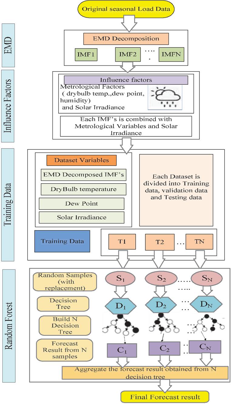
Figure 1 Framework of EMD-RF model for seasonal STLF.
3 Implementation of Proposed Model for STLF
The schematic layout of the EMD-RF approach considered for STLF is shown in Figure 1. The steps involved in the load forecast determination using EMD-RF are enlisted below:
Step 1: The decomposed IMF’s and residue are obtained using EMD from Equation (4).
Step 2: The IMF’s obtained from EMD from Step 1 is combined with multi meteorological factors dry bulb temperature, dewpoint and solar irradiance for seasonal load data. Here, relative humidity is assumed 60%.
Step 3: The dataset obtained after considering the influence factors from Step 2 is pre-processed, validated, and classified into training data set and testing data set.
Step 4: Now the training data is analysed with Random Forest technique where number of sub-samples are randomly created with replacement. The steps involved in the Random Forest (RF) are:
Step A: Create random samples from the original dataset through Bagging or Bootstrapping.
Step B: From each sample decision trees are constructed.
Step C: At each node in the decision tree, only a random set of attributes is used to determine the optimal split.
Step D: Each decision tree generates their individual prediction .
Step E: The final prediction is obtained by averaging (in regression) all of the decision trees’ predictions. .
Step 5: The final output of N decision trees obtained from Random Forest is the final result.
The detailed analysis of original six-month hourly load data of Bengaluru city (Karnataka, India) with meteorological variables (MV) and solar irradiance (SR), applied to EMD-RF model is discussed in next section.
4 Data Analysis for STLF
4.1 Analysis of Load Data
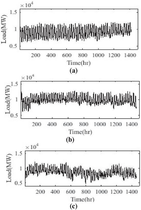
In this paper, the above EMD-RF approach is tested on real time original data of six month of Bengaluru city (Karnataka, India) from 1st January 2019 to 30th June 2019 (i.e. 181 days for 24 hours) [75], to obtain the seasonal day ahead load forecast for winter season (1st January 2019–28th February 2019), spring season (1st March 2019–30th April 2019) and summer season (1st May 2019–30th June 2019) as seen in Figure 2. As can be observed, this hourly dataset contains non-linearity and non-stationarity characteristics. Table 1 shows the results of the statistical analysis of load data. To determine the symmetry and distribution of practical data, the skewness and kurtosis are also calculated.
Figure 2 Hourly Load data (a) Winter Season (January-February), (b) Spring Season (March-April) and (c) Summer Season (May–June).
Table 1 Statistical parameters of load data
| Parameters | Winter Season | Spring Season | Summer Season |
| Minimum (MW) | 6173 | 6173 | 4690 |
| Maximum (MW) | 12012 | 12881 | 12158 |
| Mean | 9084 | 10003 | 8648 |
| Standard Error | 39 | 34 | 35 |
| Median | 8950 | 9839 | 8605 |
| St. Deviation | 1450 | 1290 | 1336 |
| Sample Variance | 2101196 | 1663367 | 1785305 |
| Kurtosis | 1.09 | 0.42 | 0.28 |
| Skewness | 0.05 | 0.04 | 0.08 |
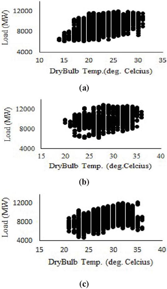
Figure 3 Load verses dry bulb temperature (a) Winter Season, (b) Spring Season, (c) Summer season.
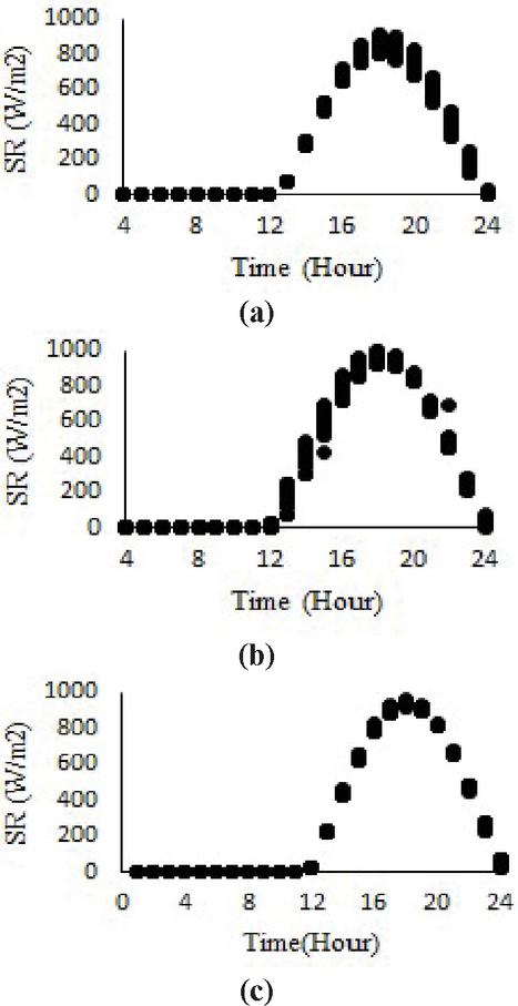
Figure 4 Solar Irradiance verses Time (a) Winter Season, (b) Spring Season, (c) Summer season.
4.2 Analysis of Meteorological Variables
The meteorological variables such as moisture content, dew point, dry bulb, and wet bulb temperature have a significant influence on forecasting future load demand owing to adverse climatic conditions. The effect of dry bulb temperature and dew point on load is shown in Figure 3(a)–(c) for winter, spring and summer seasons. The analysis of meteorological variables is tabulated in Table 1. The practical load data of Bengaluru city (Karnataka, India) is being considered, which has a distinct rainy and dry season as well as pleasant weather all year. Periodic heat waves, however, may make summer rather uncomfortable due to the negative influence of climatic circumstances. As a result, consumers are more likely to turn on the air conditioner, causing the load demand to spike in the summer. As a result, using the temperature parameter only as a major weather component in load forecasting might lead to incorrect findings. So, to estimate more improved and precise forecasting results, solar irradiance is also considered.
4.3 Analysis of Solar Irradiance
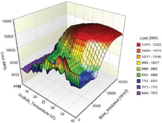
An increase and decrease in Solar Irradiance (SR) also play a significant part in climate models and weather forecasting which have a substantial influence on the energy system. The solar irradiance collected for Bengaluru city (Karnataka, India) is shown in Figure 4(a)–(c) for winter, spring and summer season. The statistical properties show that spring season shows maximum value of solar irradiance as 10443.4 W/m for, standard deviation 453.3, mean 302.14 W/m. Thus, in this case study other than dry bulb temperature, relative humidity and dew point, solar irradiance is taken into account while evaluating an accurate load forecast. Figure 5 depicts the influence of solar irradiation and dry bulb temperature on load. Table 2 shows the characteristics of meteorological data for Bengaluru city (Karnataka, India) during a six-month period.
Figure 5 Influence of dry bulb temperature and solar irradiance on load.
Table 2 Six-month meteorological Variables for Bengaluru city (Karnataka, India)
| Parameters | Jan | Feb | March | April | May | June |
| T (C) | 13 | 17 | 20 | 23 | 22 | 25 |
| T (C) | 29 | 31 | 34 | 36 | 36 | 36 |
| T (C) | 21 | 24 | 27 | 30 | 29 | 31 |
| DP (C) | 6.4 | 9.2 | 12 | 12.9 | 13.9 | 12.9 |
| DP (C) | 20.4 | 22.3 | 25.1 | 27 | 27 | 27 |
| DP (C) | 13.4 | 15.75 | 18.55 | 19.95 | 20.45 | 19.95 |
| RH (%) | 55 | 58 | 60 | 65 | 64 | 68 |
| RH (%) | 58 | 62 | 63 | 69 | 70 | 72 |
| RH(%) | 56.5 | 60 | 61.5 | 67 | 67 | 70 |
| SR (W/m) | 855.11 | 914.32 | 938.54 | 944.82 | 958.41 | 997.04 |
4.4 Data Pre-Processing
The EMD decomposition approach is used to deconstruct the six-month practical load data of Bengaluru City (Karnataka, India) from 01 January 2019 to 30 June 2019 (i.e. 181 days for 24 hours) into a finite number of IMF components. The decomposed IMF is further divided into training dataset, validation dataset and testing dataset to determine day ahead (i.e. 24 hours) STLF as tabulated in Table 3 for three consecutive seasons:
(i) Winter Season – 1st January 2019 to 28th February 2019, i.e. 59 days for 24 hours.
(ii) Spring Season – 1st March 2019 to 30th April 2019, i.e. 61 days for 24 hours.
(iii) Summer Season – 1st May 2019 to 30th May 2019, i.e. 61 days for 24 hours.
Table 3 Seasonal dataset for day ahead STLF
| S.No | Season | Training Dataset | Validation Dataset | Testing Dataset |
| 1 | Winter (January–February) | 1st January 2019 to 27th February 2019 (i.e. 57 days for 24 hours) 1368 | 27th February 2019 (i.e. 1 day for 24 hours) 24 | 28th February 2019 (i.e.1 day for 24 hours) 24 |
| 2 | Spring (March–April) | 1st March 2019 to 28th April 2019 (i.e. 59 days for 24 hours) 1416 | 29th April 2019 (i.e. 1 day for 24 hours) 24 | 30th April 2019 (i.e. 1 day for 24 hours) 24 |
| 3 | Summer (May–June) | 1st May 2019 to 28th June 2019 (i.e. 29 days for 24 hours) 1416 | 29th June 2019 (i.e. 1 day for 24 hours) 24 | 30th June 2019 (i.e. 1 day for 24 hours) 24 |
4.5 Assessment Indicators
The appropriate selection of forecasting error indicators is essential for evaluating the model’s performance. In addition to the simulation plots, the suggested model’s performance is evaluated using five evaluation criteria: Mean Absolute Error (MAE), Root Mean Square Error (RMSE), Relative Root Mean Square Error (RRMSE), and Mean Absolute Percentage Error (MAPE), whose expressions are:
(i) Mean Absolute Error (MAE)
| (12) |
(ii) Root Mean Square Error (RMSE)
| (13) |
(iii) Relative Root Mean Square Error (RRMSE)
| (14) |
(iv) Mean Absolute Percentage Error (MAPE)
| (15) |
Where is the number of samples, is the forecasted value, and is the actual value. The smaller these assessment indicators’ values are, the more exact and accurate the outcomes will be.
5 Result Analysis and Discussion
5.1 Simulation Settings
The simulation of proposed EMD-RF model for STLF is carried out in two steps: (i) Firstly, EMD method is applied to decompose practical load data into IMF’s and residue. (ii) Secondly, Random Forest model is constructed on the parameters given in Table 4.
Table 4 Simulation settings for random forest model
| Model | Parameters |
| Random Forest | Number of Trees N |
| Number of candidate variables in each split 3 | |
| Minimum Node size 5 |
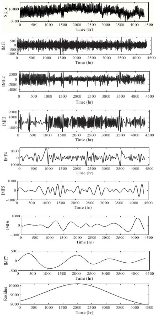
Figure 6 EMD results for six-month load data.
5.2 Decomposition of Practical Load Data
The six-month practical load data of Bengaluru City (Karnataka, India) is first analysed using EMD approach. Figure 6 shows the EMD decomposition of the practical data into seven IMF’s and one residue. The decomposed IMF’s are combined with meteorological variables. Afterwards proposed hybrid model is implemented using Random Forest (RF) on these IMF’s to obtain accurate and precise results.
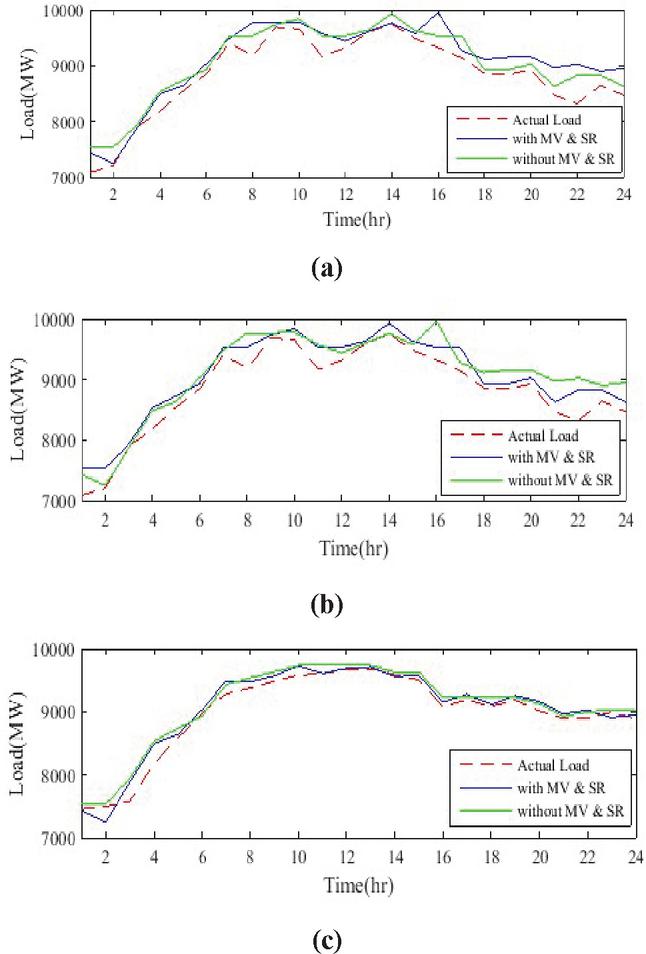
Figure 7 Actual load vs Forecasted load based on EMD-RF model considering with and without the effect of MV and SR (a) Winter season (January–February), (b) Spring season (March–April) and (c) Summer season (May–June).
5.3 Model Forecasting Results
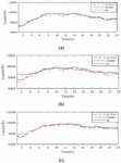
The STLF technique based on EMD-RF model is evaluated for day ahead winter, spring and summer season. Figure 7 represents day ahead STLF considering with and without the influence of meteorological variables (MV) and solar irradiance (SR) for various seasons. The statistical parameters estimated for EMD-RF model with and without meteorological variables (MV) and solar irradiance (SR) for day ahead forecasted load is tabulated in Table 5. The statistical error estimation shows that when influence factors is taken into consideration the MAPE obtained for winter season is 2.02%, spring season is 2.10% and summer season is 2.09%, and MAE estimated for winter season is 208.45 MWh, spring season is 215.63 MWh and summer season is 177.13 MWh which is minimum in comparison when influence factors are not taken into account.
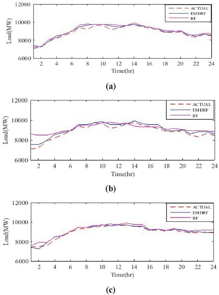
To obtain the clear picture, the comparison between proposed EMD-RF approach with Random Forest (RF) technique is also analysed and depicted in Figure 8 to confirm the efficiency of proposed approach. The error metrics evaluated for RF technique yields MAPE for winter season is 2.54%, spring season is 3.59% and summer season is 2.47% and MAE for winter season is 215.29 MWh, spring season is 340.46 MWh and summer season is 197.59 Mwh which is more when compared with EMD-RF model as shown in Table 6.
Table 5 Statistical Error evaluation of day ahead STLF with EMD-RF approach for various seasons
| Winter (January–February) | Spring (March–April) | Summer (May–June) | |||||
| S.No | Error Parameters | With MV and SR | Without MV and SR | With MV and SR | Without MV and SR | With MV and SR | Without MV and SR |
| 1 | MAE (MWh) | 208.45 | 310.12 | 215.63 | 265 | 177.13 | 222.7 |
| 2 | RMSE (MWh) | 222.57 | 335.31 | 224.25 | 275.83 | 198.78 | 449.37 |
| 3 | RRMSE (%) | 2.12 | 3.2 | 2.13 | 2.61 | 2.05 | 5.18 |
| 4 | MAPE (%) | 2.02 | 3.3 | 2.1 | 2.58 | 2.09 | 2.63 |
5.4 Comparative Analysis with Various Forecasting Models
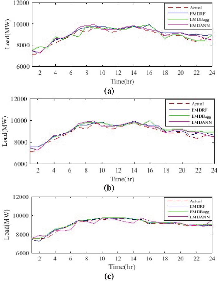
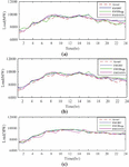
The result obtained from the EMD-RF model is compared and evaluated with other non-decomposition based methods such as Artificial Neural Network (ANN), Bagging and Random Forest (RF) and decomposition method based combined models such as EMD-ANN and EMD-Bagging to prove the efficiency of the approach considering the effect of meteorological variables (MV) and solar irradiance (SR). Figure 9(a)–(c) depicts a visual comparison of actual load and forecasted load based on EMD methods such as EMD-RF,
Figure 8 Actual load vs Forecasted load based on EMD-RF and RF model considering the effect of MV and SR (a) Winter season (January–February), (b) Spring season (March–April) and (c) Summer season (May–June).
Table 6 Statistical Error evaluation of day ahead STLF with EMD-RF and RF technique for various seasons
| Winter (January–February) | Spring (March–April) | Summer (May–June) | |||||
| S.No | Error Parameters | EMD-RF | RF | EMD-RF | RF | EMD-RF | RF |
| 1 | MAE (MWh) | 208.45 | 215.29 | 215.63 | 340.46 | 177.13 | 197.59 |
| 2 | RMSE (MWh) | 222.57 | 226.63 | 224.25 | 398.03 | 177.78 | 239.04 |
| 3 | RRMSE (%) | 2.12 | 2.74 | 2.13 | 4.06 | 2.05 | 2.88 |
| 4 | MAPE (%) | 2.02 | 2.54 | 2.1 | 3.59 | 2.09 | 2.47 |
EMD-Bagging and EMD-ANN taking into account the influence of meteorological factors and solar irradiance for various seasons. The representation of quantative assessment of day ahead STLF for different techniques is tabulated in Table 7 for winter season, spring season and summer.
Figure 9 Comparison between Actual Load vs Forecasted load considering the effect of meteorological variables (MV) and solar irradiance (SR) based on EMD-RF, EMD-Bagging, EMD-ANN (a) Winter Season (January–February) (b) Spring Season (March–April), (c) Summer Season (May–June).
Table 7 Quantitative assessment of various techniques for day ahead STLF for winter, spring and summer
| Error | MAE (MWh) | RMSE (MWh) | RRMSE (%) | MAPE (%) | |||||||||
| Seasons | |||||||||||||
| S.No. | Methods | Winter | Spring | Summer | Winter | Spring | Summer | Winter | Spring | Summer | Winter | Spring | Summer |
| 1 | ANN | 280.31 | 341.84 | 399.13 | 317.98 | 410.87 | 478 | 4.37 | 4.16 | 4.85 | 3.91 | 3.76 | 4.09 |
| 2 | Bagging | 238.79 | 351.31 | 230.67 | 248.98 | 403.03 | 258.4 | 3.35 | 4.12 | 3.11 | 3.37 | 3.65 | 2.89 |
| 3 | RF | 218.92 | 340.46 | 197.59 | 239.59 | 398.03 | 239.04 | 2.89 | 4.06 | 2.88 | 2.74 | 3.59 | 2.47 |
| 4 | EMD-ANN | 256.06 | 234.86 | 197.75 | 265.11 | 234.93 | 216.63 | 2.75 | 2.25 | 2.58 | 2.72 | 2.28 | 2.33 |
| 5 | EMD-Bagging | 237.83 | 260.97 | 180.09 | 241.43 | 272.44 | 224.25 | 2.5 | 2.58 | 2.64 | 2.53 | 2.54 | 2.62 |
| 6 | EMD-RF | 208.45 | 215.63 | 177.13 | 222.57 | 224.25 | 178.59 | 2.12 | 2.13 | 2.13 | 2.02 | 2.1 | 2.1 |
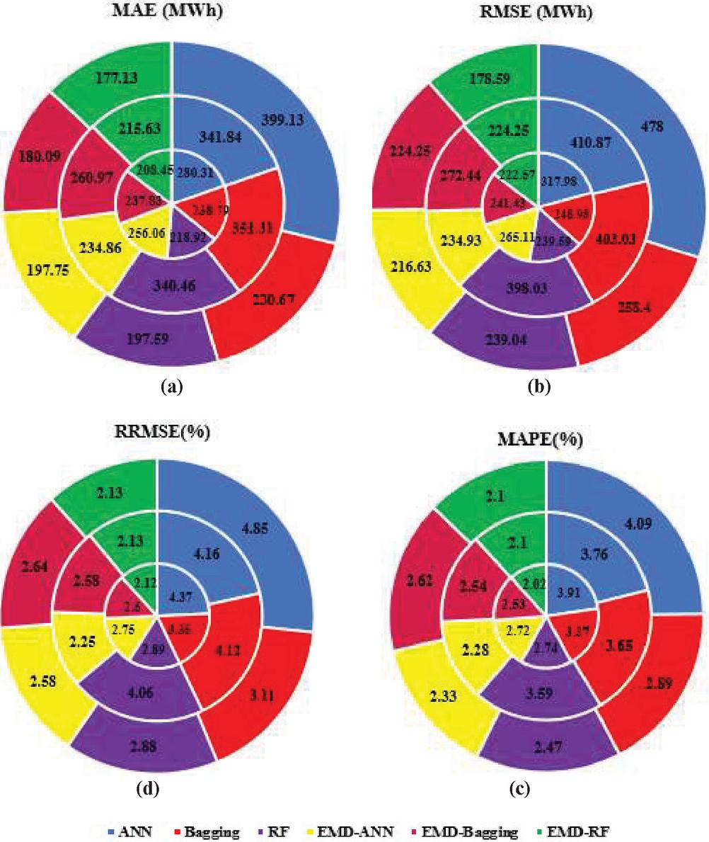
Figure 10 Comparison between MAE, RMSE, RRMSE and MAPE of various techniques for day ahead STLF for winter season, spring season and summer season.
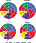
The pie chart is used to display the MAE, MAPE, RMSE and RRMSE for comparative analysis between various techniques as depicted in Figure 10(a)–(d). The inner wheel of pie chart represents the error values of winter season, middle wheel represents the error estimation of spring season and outer wheel represents the error values of summer season. The result shows that, for winter and summer season MAE obtained for ANN is 280.31 MWh and 399.13 MWh whereas for spring season MAE is 351.31 MWh which is more in comparison to other techniques. The RMSE obtained for EMD-ANN yields 265.11 MWh and ANN yields 317.98 MWh in winter season, in spring season EMD-Bagging produces RMSE 271.44 MWh and ANN produces RMSE 410.87 MWh and in summer season RF estimates RMSE 239.04 MWh and ANN estimates RMSE 478 MWh which is large in comparison to other techniques. The MAPE estimated in winter for EMD-ANNN and ANN is 3.91% and 2.74% whereas in spring and summer season EMD-Bagging yields MAPE 2.54% and 2.62% and ANN yields MAPE 3.76% and 4.09% which is maximum when compared to all decomposition and mon-decomposition methods.
Thus, for practical six month hourly load data of Bengaluru city (Karnataka, India), the results obtained from the proposed hybrid model based on the EMD-RF method demonstrate enhanced performance and accuracy with minimum error variability in forecasting, resulting in optimal cost savings and better load scheduling in the energy utility and power system.
6 Conclusion
In this study, a decomposition-based EMD approach is suggested and implemented for short-term load forecasting using the Random Forest (RF) methodology on real-time seasonal load data from Bengaluru (Karnataka, India) for six months, with and without the influence of multi-meteorological factors. The conclusion regarding the results of these results are summarized as below:
• The proposed hybrid model EMD-RF successfully forecasts the day ahead of a load of practical load data with a minimum error when meteorological data is considered as compared to the load forecasted when meteorological data is not considered with a hybrid model.
• Other decomposition and ensemble-based STLF approaches such as EMD-Bagging, EMD-ANN, Bagging, and Random Forest are compared to the evaluated forecasted results achieved by the proposed hybrid model. The statistical analysis reveals that the suggested hybrid model for STLF improves performance and produces better outcomes.
As a consequence of the quantitative error measurements, the suggested hybrid EMD -RF model is recommended as an alternative strategy for improved STLF. The suggested hybrid model’s anticipated load provides great forecasting performance and superior outcomes when compared to other approaches that take into consideration the influence of meteorological data, hence enhancing the electric power utility.
Acknowledgement
The author wishes to express her appreciation to Late Dr. Stuti Shukla Datta, Assistant Professor, Amity University Uttar Pradesh, Lucknow campus, who made significant contributions to the completion of this research project, as well as assisting the author in broadening her research area.
References
[1] Y. Al-Rashid and L.D. Paarmann, “Short-term electric load forecasting using neural network models,” Circuits and Syst., Ames, IA, 1996, pp. 1436–1439.
[2] Medha Joshi, Rajiv Singh, “Short-term load forecasting approaches: A review”, International Journal of Recent Engineering Research and Development (IJRERD) Volume No. 01 – Issue No. 03, ISSN: 2455-8761, pp. 09–17.
[3] Swarpoor R., Hussien A. Abdelqader, “load forecasting for power system planning and operation using artificial neural network at albatinah region oman,” Journal of Engineering Science and Technology Vol. 7, No. 4 (2012) 498–504.
[4] G. T. Heinemann, D. A. Nordmian, E. C. Plant. “The relationship between summer weather and summer loads – a regression analysis”, IEEE Transactions on Power Apparatus and Systems, vol. PAS-85, no. 11, pp. 1144–1154, Nov. 1966.
[5] Comparison of conventional and modern load forecasting techniques based on artificial intelligence and expert systems, IJCSI International Journal of Computer Science Issues, Vol. 8, Issue 5, No 3, September 2011 ISSN (Online): 1694–0814.
[6] Tao Hong, David A. Dickey.: Electric load forecasting: fundamentals and best practices (2009).
[7] J. H. Park, Y. M. Park and K. Y. Lee, “Composite Modeling for Adaptive Short-Term Load Forecasting,” IEEE Transaction Power System, vol. 6, no. 2, pp. 450–457, May 1991.
[8] H. M. Al-Hamadi and S. A. Soliman, “Long-term/mid-term electric load forecasting based on short-term correlation and annual growth,” Electr. Power Syst. Res., vol. 74, no. 3, pp. 353–361, 2005.
[9] S. Farzana, M. Liu, A. Baldwin, and M. U. Hossain, “Multi-model prediction and simulation of residential building energy in urban areas of Chongqing, South West China,” Energy Build., vol. 81, pp. 161–169, Oct. 2014.
[10] R. P. Broadwater, A. Sargent, A. Yarali, H. E. Shaalan and J. Nazarko, “Estimating Substation Peaks from Research Data, IEEE Transaction on Power Delivery, vol. 12, pp. 451–456, 1997.
[11] S. G. N and G. S. Sheshadri, 2020, Electrical Load Forecasting Using Time Series Analysis, IEEE Bangalore Humanitarian Technology Conference (B-HTC), Vijiyapur, India, 2020, pp. 1–6, doi: 10.1109/B-HTC50970.2020.9297986.
[12] B. Nepal, M. Yamaha, A. Yokoe, T. Yamaji, 2020, Electricity load forecasting using clustering and ARIMA model for energy management in buildings. JpnArchit Rev.; 3: 62–76. https://doi.org/10.1002/2475-8876.12135.
[13] S. J. Huang and K. R. Shih, 2003, Short-term load forecasting via ARMA model identification including non-Gaussian process considerations, IEEE Trans. Power Syst., vol. 18, no. 2, pp. 673–679, May 2003.
[14] J. Y. Fan and J. D. McDonald, “A real-time implementation of short term load forecasting for distribution power systems,” IEEE Trans. Power Syst., vol. 9, no. 2, pp. 988–994, May 1994.
[15] Marco Cococcioni, Eleonora D’Andrea and Beatrice Lazzerini “One day-ahead forecasting of energy production in solar photovoltaic installations: An empirical study,” Intelligent Decision Technologies 6, pp. 197–210, 2012.
[16] Mandeep Singh, Raman Maini, “Various Electricity Load Forecasting Techniques with Pros and Cons”, International Journal of Recent Technology and Engineering (IJRTE) ISSN: 2277–3878, Volume-8 Issue-6, March 2020.
[17] G. Dudek, P. Pełka and S. Smyl, 2020, A Hybrid Residual Dilated LSTM and Exponential Smoothing Model for Midterm Electric Load Forecasting, in IEEE Transactions on Neural Networks and Learning Systems, doi: 10.1109/TNNLS.2020.3046629.
[18] Taylor, J.W., 2003. “Short-term electricity demand forecasting using double seasonal exponential smoothing,” Journal of the Operational Research Society, 44(0): 799–805.
[19] Taylor, J.W., 2012. “Short-Term Load Forecasting With Exponentially Weighted Methods,” IEEE Transactions on Power Systems, 27(1): 458–464.
[20] McKenzie, E. and E.S. Gardner Jr, 2010. “Damped trend exponential smoothing: A modelling viewpoint,” International Journal of Forecasting, 26(4): 661–665.
[21] Ming-Guang Zhang, “Short-term load forecasting based on support vector machines regression,” 2005 International Conference on Machine Learning and Cybernetics, Guangzhou, China, 2005, pp. 4310–4314 Vol. 7, doi: 10.1109/ICMLC.2005.1527695.
[22] M. S. Li, J. L. Wu, T. Y. Ji, Q. H. Wu and L. Zhu, “Short-term load forecasting using Support Vector Regression-based Local Predictor,” 2015 IEEE Power & Energy Society General Meeting, Denver, CO, 2015, pp. 1–5, doi: 10.1109/PESGM.2015.7285911.
[23] L. Hu, L. Zhang, T. Wang and K. Li, 2020, Short-term load forecasting based on support vector regression considering cooling load in summer, 2020 Chinese Control and Decision Conference (CCDC), Hefei, China, pp. 5495–5498, doi: 10.1109/CCDC49329.2020.9164387.
[24] Chia-Nan Ko and Cheng-Ming Lee. Short-term load forecasting using SVR (support vector regression)-based radial basis function neural network with dual extended kalman filter. Energy, 49:413–422, 2013.
[25] Glauber Souto dos Santos, Luiz Guilherme Justi Luvizotto, Viviana Cocco Mariani, and Leandro dos Santos Coelho. Least squares support vector machines with tuning based on chaotic differential evolution approach applied to the identification of a thermal process. Expert Systems with Applications, 39(5):4805–4812, 2012.
[26] T. Czernichow, A. Piras, K. Imhof, P. Caire, Y. Jaccard, B. Dorizzi, and A. Germond, “Short term electrical load forecasting with artificial neural networks,” Engineering Intelligent Syst., vol. 2, pp. 85–99, 1996.
[27] Peng T, Hubele N, Karady G. Advancement in the application of neural networks for short term load forecasting. IEEE Trans Power Syst 1992;7(1):250–8.
[28] Yao S, Song Y, Zhang L, Cheng X. Wavelet transform and neural networks for short term electrical load forecasting. Energ Convers Manage 2000;41:1975–88.
[29] Tang, X., Dai, Y., Wang, T. and Chen, Y., 2019, Shortterm power load forecasting based on multi-layer bidirectional recurrent neural network. IET Gener. Transm. Distrib., 13: 3847–3854. https://doi.org/10.1049/iet-gtd.2018.6687.
[30] Muhammad Buhari and Sunusi Sani Adamu, “Short-Term Load Forecasting Using Artificial Neural Network,” International Multi Conference of Engineers and Computer Scientists., vol. 1, pp. 442–449, March 2012.
[31] Huang, C-J, Shen, Y, Chen, Y-H, Chen, H-C. A novel hybrid deep neural network model for short-term electricity price forecasting. Int J Energy, Res. 2021; 45: 2511–2532. https://doi.org/10.1002/er.5945
[32] Arjun Baliyan, Kumar Gaurav and Sudhansu Kumar Mishra, “A Review of Short Term Load Forecasting using Artificial Neural Network Models,” Procedia Computer Science, 2015, vol. 48, pp. 121–125.
[33] Srashti Shrivastava and Dr. Krishna Teerth Chaturvedi, “A Review of Artificial Intelligence Techniques for Short Term Electric Load Forecasting,” International Journal of Advanced Research in Electrical, Electronics and Instrumentation Engineering, Vol. 7, Issue 5, pp. 2241–2247, May 2018.
[34] Mastorocostas P, Theocharis J, Kiartzis S, Bakirtzis A. A hybrid fuzzy modeling method for short-term load forecasting. Math Comput Simulat 2000;51:221–32.
[35] Sokratis Papadopoulos, Ioannis Karakatsanis, “Short-term Electricity Load Forecasting using Time Series and Ensemble Learning Methods”, publication/282939702, March 2015.
[36] Melih Yucesan, Engin Pekel, Erkan Celik, Muhammet Gul and Faruk Serin (2021) Forecasting daily natural gas consumption with regression, time series and machine learning based methods, Energy Sources, Part A: Recovery, Utilization, and Environmental Effects, DOI: 10.1080/15567036.2021.1875082.
[37] Sewell, M. Ensemble Learning; Technical Report; University College London: London, UK, 2008.
[38] Zhou, Z.H. Ensemble Methods: Foundations and Algorithms, 1st ed.; Chapman & Hall CRC: Boca Raton, FL, USA, 2012.
[39] Zhang, C.; Ma, Y. Ensemble Machine Learning: Methods and Applications; Springer Science & Business Media: Boston, MA, USA 2012.
[40] Hakan Acikgoz, Ceyhun Yildiz and Mustafa Sekkeli (2020) An extreme learning machine based very short-term wind power forecasting method for complex terrain, Energy Sources, Part A: Recovery, Utilization, and Environmental Effects, 42:22, 2715–2730, DOI: 10.1080/15567036.2020.1755390.
[41] Breiman, L. (1996b) Bagging predictors. Machine Learning, vol. 24, no. 2, pp. 123–140.
[42] J. Vaish, S. S. Datta and K. Seethalekshmi, 2020, Short Term Load Forecasting using ANN and Ensemble Models Considering Solar Irradiance, IEEE International Conference on Electrical and Electronics Engineering (ICE3), Gorakhpur, India, pp. 44–48, doi: 10.1109/ICE348803.2020.9122986.
[43] J. Vaish, S. S. Datta and k. Seethalekshmi, 2021, Short-term Load Forecasting using Bootstrap Aggregation based Ensemble Method, IEEE 7th International Conference on Electrical Energy Systems (ICEES), Chennai, India, pp. 245–249, doi: 10.1109/ICEES51510.2021.9383755.
[44] Grzegorz Dudek, “Short-Term Load Forecasting Using Random Forests”, Intelligent Systems’2014: Proceedings of the 7th IEEE International Conference Intelligent Systems IS’2014, September 24–26, 2014, Warsaw, Poland, Volume 2: Tools, Architectures, Systems, Applications (pp. 821–828).
[45] A. Lahouar, J. Ben Hadj Slama, “Day-ahead load forecast using random forest and expert input selection”, Energy Conversion and Management; ISSN 0196–8904; Worldcat; 2015; v. 103; pp. 1040–1051.
[46] Federico Divina, Aude Gilson, Francisco Goméz-Vela, Miguel García Torres and José F. Torres, “Stacking Ensemble Learning for Short-Term Electricity Consumption Forecasting,” energies 2018, MDPI, Published: 16 April 2018, pp. 1–31.
[47] T. H. Cormen, C. E. Leiserson, R. L. Rivest, and C. Stein, Introduction to Algorithms. MIT Press, 2000.
[48] C. Guan, P. B. Luh, L. D. Michel, Y. Wang, and P. B. Friedland, “Very short-term load forecasting: wavelet neural networks with data prefiltering,” IEEE Transactions on Power Systems, vol. 28, no. 1, pp. 30–41, 2013.
[49] R.-A. Hooshmand, H. Amooshahi, and M. Parastegari, “A hybrid intelligent algorithms based short-term load forecasting approach,” International Journal of Electrical Power & Energy Systems, vol. 45, pp. 313–324, 2013.
[50] N. E. Huang, Z. Shen, S. R. Long, M. C. Wu, H. H. Shih, Q. Zheng, N.- C. Yen, C. C. Tung, and H. H. Liu, “The empirical mode decomposition and the hilbert spectrum for nonlinear and non-stationary time series analysis,” in Roy. Soc. London A, vol. 454, 1998, pp. 903–995.
[51] M. Alhamdoosh and D. Wang, “Fast decorrelated neural network ensembles with random weights,” Information Sciences, vol. 264, pp. 104–117, 2014.
[52] X. Zhang, K. K. Lai, and S.-Y. Wang, “A new approach for crude oil price analysis based on Empirical Mode Decomposition,” Energy Economics, vol. 30, no. 3, pp. 905–918, 2008.
[53] M. Hu and H. L. Liang, “Adaptive multiscale entropy analysis of multivariate neural data,” IEEE Transactions on Biomedical Engineering, vol. 59, no. 1, pp. 12–15, 2012.
[54] Y. Wei and M.-C. Chen, “Forecasting the short-term metro passenger flow with empirical mode decomposition and neural networks,” Transportation Research Part C: Emerging Technologies, vol. 21, no. 1, pp. 148–162, 2012.
[55] J. Wang, W. Zhang, Y. Li, J. Wang, and Z. Dang, “Forecasting wind speed using empirical mode decomposition and ELMAN neural network,” Applied Soft Computing, vol. 23, pp. 452–459, 2014.
[56] C.-F. Chen, M.-C. Lai, and C.-C. Yeh, “Forecasting tourism demand based on empirical mode decomposition and neural network,” Knowledge-Based Systems, vol. 26, pp. 281–287, 2012.
[57] Z.-H. Zhu, Y.-L. Sun, and Y. Ji, “Short-term load forecasting based on EMD and SVM,” High Voltage Engineering, vol. 33, no. 5, pp. 118–122, 2007.
[58] C. S. Lai et al., 2020, “Multi-view Neural Network Ensemble for Short and Mid-term Load Forecasting,” in IEEE Transactions on Power Systems, doi: 10.1109/TPWRS.2020.3042389.
[59] L. Wang, S. Mao and B. Wilamowski, 2019, Short-Term Load Forecasting with LSTM Based Ensemble Learning, International Conference on Internet of Things (iThings) and IEEE Green Computing and Communications (GreenCom) and IEEE Cyber, Physical and Social Computing (CPSCom) and IEEE Smart Data (SmartData), pp. 793–800, doi: 10.1109/iThings/GreenCom/CPSCom/SmartData.2019.00145.
[60] Z. Tang, G. Zhao, G. Wang and T. Ouyang, 2020, “Hybrid Ensemble Framework for Short-Term Wind Speed Forecasting,” in IEEE Access, vol. 8, pp. 45271–45291, doi: 10.1109/ACCESS.2020.2978169.
[61] J. Bedi and D. Toshniwal, 2018, Empirical Mode Decomposition Based Deep Learning for Electricity Demand Forecasting, IEEE Access, vol. 6, pp. 49144–49156, doi: 10.1109/ACCESS.2018.2867681.
[62] Fan, G-F, Guo, Y-H, Zheng, J-M, Hong, W-C., 2020, A generalized regression model based on hybrid empirical mode decomposition and support vector regression with back-propagation neural network for mid-short-term load forecasting. Journal of Forecasting; 39: 737–756. https://doi.org/10.1002/for.2655
[63] H. Jun et al., 2020, A Novel Short-term Residential Load Forecasting Model Combining Machine Learning Method with Empirical Mode Decomposition, Asia Energy and Electrical Engineering Symposium (AEEES), Chengdu, China, pp. 816–820, doi: 10.1109/AEEES48850.2020.9121467.
[64] S. Fan, L. Chen and W. Lee, 2009, Short-Term Load Forecasting Using Comprehensive Combination Based on Multi meteorological Information, IEEE Transactions on Industry Applications, vol. 45, no. 4, pp. 1460–1466, July-Aug., doi: 10.1109/TIA.2009.2023571.
[65] W. Chu, Y. Chen, Z. Xu and W. Lee, “Multiregion Short-Term Load Forecasting in Consideration of HI and Load/Weather Diversity,” in IEEE Transactions on Industry Applications, vol. 47, no. 1, pp. 232–237, Jan.-Feb. 2011, doi: 10.1109/TIA.2010.2090440.
[66] Takilalte, S. Harrouni and J. Mora (2019) Forecasting global solar irradiance for various resolutions using time series models – case study: Algeria, Energy Sources, Part A: Recovery, Utilization, and Environmental Effects, DOI: 10.1080/15567036.2019.1649756.
[67] Song Li, Lalit Goel, Peng Wang, 2016, An ensemble approach for short-term load forecasting by extreme learning machine, Applied Energy, Volume 170, Pages 22–29, ISSN 0306–2619, https://doi.org/10.1016/j.apenergy.2016.02.114.
[68] Z.-H. Zhou, 2012, Ensemble Methods: Foundations and Algorithms. Boca Raton, FL: Chapman and Hall/CRC.
[69] P. Kumkar, I. Madan, A. Kale, O. Khanvilkar and A. Khan, 2018, Comparison of Ensemble Methods for Real Estate Appraisal, IEEE 3rd International Conference on Inventive Computation Technologies (ICICT), Coimbatore, India, pp. 297–300, doi: 10.1109/ICICT43934.2018.9034449.
[70] Angel Colmenares and Jianzhou Wang (2021) Double ensemble system for wind energy forecasting based on generalized autoregressive conditional heteroskedasticity and neural network models with variational mode decomposition, Energy Sources, Part A: Recovery, Utilization, and Environmental Effects, DOI: 10.1080/15567036.2021.1922550.
[71] Ying-Ying Cheng, P. P. K. Chan and Zhi-Wei Qiu, 2012, Random forest-based ensemble system for short term load forecasting, International Conference on Machine Learning and Cybernetics, pp. 52–56, doi: 10.1109/ICMLC.2012.6358885.
[72] Xiaoyu Wu, Jinghan He, Tony Yip, Jian lu and Ning Lu, “A two-stage random forest method for short-term load forecasting,” 2016 IEEE Power and Energy Society General Meeting (PESGM), 2016, pp. 1–5, doi: 10.1109/PESGM.2016.7741295.
[73] Breiman, L., Friedman, J.H., Olshen, R.A., Stone, C.J., 1984: Classification and Regression Trees. Chapman and Hall (1984).
[74] Y. Xuan et al.,2021, Multi-Model Fusion Short-Term Load Forecasting Based on Random Forest Feature Selection and Hybrid Neural Network, IEEE Access, vol. 9, pp. 69002–69009, 2021, doi: 10.1109/ACCESS.2021.3051337.
[75] Website Online: http://218.248.45.137:8282/LoadCurveUpload/lcdownloadview.asp
Biographies

Jayati Vaish received B. Tech degree from Integral University, Lucknow, Uttar Pradesh India in 2008 and Master’s degree from IIT Roorkee, Uttrakhand, India in 2013. From 2013 to 2017 she was working as Assistant Professor in Shri Ram Swaroop Group of Professional Colleges, Lucknow, Uttar Pradesh, India. Since 2018 she is working as a PhD Research Scholar in Amity University, Lucknow Campus, Uttar Pradesh, India. She has received the Best Project award in Electrical Engineering. Her area of interest includes Load Forecasting, Micro-Grid Generation scheduling, Electric Vehicles.

Anil Kumar Tiwari received B.Tech. from Thapar University, Patiala, India and Master’s degree from Pune University, India and Ph.D. degree in Electrical engineering from MNIT Allahabad, Uttar Pradesh, India. Since 2011 he is working as Director of AMITY School of Engineering AMITY University Uttar Pradesh Lucknow Campus, India. He holds more than three decades of experience as a practicing engineer, researcher and academic administrator. He has chaired numerous International and National Conferences and won numerous Best paper awards in India and abroad.

Seethalekshmi K. received B.Tech. from Regional Engineering College, Calicut, Kerala in 1991 and Master’s degree from College of Engineering, Trivandrum, Kerala, India in 1996 and Ph.D. degree in Electrical engineering from IIT Kanpur, Uttar Pradesh, India, in 2011. From 2011 to 2016, she was working as Professor in BBDNITM, Lucknow, Uttar Pradesh, India. Since 2017, she has been Professor in Electrical Engineering Department, IET, Lucknow, U.P., India. She is the author of many Journals and also POSCO awardee. Her research interests include Power system dynamics and control, Power system protection.
Distributed Generation & Alternative Energy Journal, Vol. 37_4, 1159–1190.
doi: 10.13052/dgaej2156-3306.37411
© 2022 River Publishers
