Wind Power Deviation Charge Reduction using Machine Learning
Sandhya Kumari1, Sreenu Sreekumar2,*, Sonika Singh1 and D. P. Kothari3
1EECD, DIT University, Dehradun, India
2National Institute of Technology, Silchar, India
3THDC Institute of Hydropower Engineering and Technology, Uttarakhand, India
E-mail: 1000014598@dit.edu.in; sreenu@ee.nits.ac.in; sonika.singh@dituniversity.edu.in; dpkvits@gmail.com
*Corresponding Author
Received 03 May 2022; Accepted 01 August 2023; Publication 02 November 2023
Abstract
High penetration of wind power plants in power systems resulted in various challenges such as frequent system imbalances due to highly uncertain and variable wind generation. Additional spinning reserves and specific balancing products such as flexible ramp products are used to handle such frequent imbalances. Incorporation of these ancillary services leads to increased total operational costs. Increased operational costs should be transferred to wind power producers as it is caused by wind power plants. This leads to penalizing the wind power producers for the deviation of power generation from forecasts, called deviation charges. These deviation charges can be reduced by improving the forecasting accuracy. Existing forecasting models show performance in terms of error matrices. Such error matrices do not indicate the financial loss associated with it. This can be overcome by expressing forecasting performance in terms of deviation charge and it will directly encourage wind power producers to improve forecasting accuracy or arrange reserves to accommodate the error. This paper proposes a backpropagation-based artificial neural network model for reducing deviation charges in this context. An analysis is conducted on the data collected from the Bonneville Power Administration (BPA) Balancing Area. Seasonal analysis (Spring, Summer, Fall, and Winter) is conducted to show the performance of the proposed model throughout the year. The proposed model performance is compared with linear regression and ARIMA models. The comparison shows that the proposed ANN model gives the least deviation charges in the Spring, Summer, and Winter seasons and deviation charges in the Fall season are higher than the ARIMA model.
Keywords: ARIMA, artificial neural networks, deviation charges, linear regression, power system planning, renewable integration, wind power generation.
1 Introduction
Power systems have been experiencing very high renewable energy integration to tackle adverse climate changes [12, 27, 17]. Wind and solar generation dominate these renewables due to their widespread availability and low-cost matured technologies [13]. Wind generation shows higher uncertainty than solar generation, resulting in various operational challenges such as frequent system imbalances [14]. Additional spinning reserves and specific balancing products like flexible ramp products are used to handle such frequent system imbalances [23]. Sometimes times system needs extra generation due to lower wind generation than expected and other times the system needs to reduce its generation due to extra wind generation than expected. Ancillary services are used to handle such situations. These ancillary services increase total system operating costs [14]. Increased operation cost is usually transferred to the wind power producers as it is caused by them. Therefore, wind power producers are penalized for not providing (or providing extra power than) the committed power. The penalty depends on the deviation of wind power forecasts from actual generation [24]. These penalties are called deviation charges.
Deviation charges can be reduced by improving the accuracy of wind power forecasts [24]. Forecasting accuracy can be enhanced by selecting suitable forecasting models [28]. Wind power forecasting got quantum research attention due to its importance in power system operation planning [25, 30, 29]. However, most of the existing wind power forecasting studies represent forecasting performance in terms of various error matrices such as Mean Absolute Error (MAE, MW), Mean Square Error (MSE, ), and Mean Absolute Percentage Error (MAPE, %) [6]. These error matrices do not provide the direct financial impacts of forecasting accuracy. Representing forecasting performance in terms of financial impacts motivates wind power producers to improve their forecasts for profit maximization. This necessitates forecasting performance evaluation in terms of financial impacts such as deviation charges. There is only a little attention towards deviation charge-based forecasting performance evaluation [15, 3, 18, 5].
Most of the system operations like real-time economic dispatch and power system flexibility requirement evaluations are done in very short time frames like 5/15/30/60 minute wise [23]. Power system operational time frames have been continuously reduced over the period to handle the uncertain variability of renewable generation [22]. Therefore, deviation charge estimation with a high resolution like five minutes is required. Several models such as Numerical Weather prediction [19], time series [7], machine learning [25], probabilistic [26], and hybrid [21] are mainly used for very short-term wind power forecasting. However, all these studies show forecasting performance in terms of error matrices and do not provide any direct indication of the financial impacts of forecasts.
In this context, this paper proposes a very short-term back propagation-based ANN forecasting model for deviation charge reduction. An analysis is conducted on five-minute-wise wind generation data collected from the Bonneville Power Administration (BPA) balancing area. The seasonal analysis is conducted to analyze the performance throughout the year. Spring, Summer, Fall, and Winter seasons are selected for analysis. Multi-variable linear regression and ARIMA models are also implemented along with ANN for comparison. Results show that the proposed back propagation-based ANN model shows the least deviation charges in the Spring, Summer, and Winter seasons and the ARIMA model shows the least deviation charges in the Fall season. Forecasting performance expressed in deviation charges may motivate wind power providers to enhance forecasting accuracy further and it helps them to achieve maximum profits.
The rest of the paper is organized as follows: Section 2 discusses the mathematical modeling of the proposed very short-term back-propagation-based ANN, multi-variable linear regression, and ARIMA models. Section 3 explains the equations used for deviation charge estimation. Section 4 gives the results and discussions of seasonal analysis. Section 5 concludes that the proposed ANN model offers the least annual deviation compared to reference models.
2 Mathematical Modeling of ANN and Reference Models
Mathematical modeling of proposed very short-term back-propagation-based ANN, ARIMA, and multi-linear regression are given in this section. ARIMA and multi-linear regression models are used as reference models for deviation charge comparison.
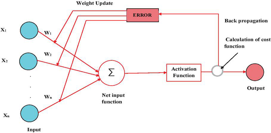
Figure 1 Feed-forward backpropagation ANN model.
Figure 2 Weight adjustments in back propagation based ANN model.
2.1 Back-propagation Based ANN Model
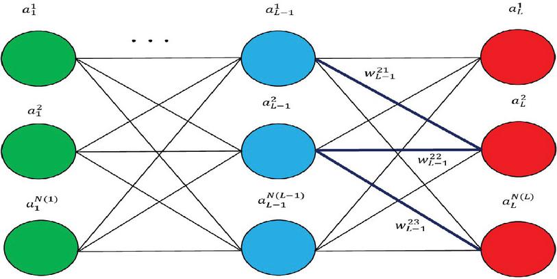
Artificial Neural Networks (ANN) learn from the training data. The learning process uses training inputs and outputs. It continuously changes model parameters (called weights) during learning. It gives output for various inputs using finalized parameters after training. ANN models are widely used in various applications like mapping, pattern recognition, and forecasting. Several types of ANN models such as back-propagation-based ANN are available [10]. Back-propagation-based ANN is suitable for forecasting due to its superior learning capabilities. Back-propagation-based ANN is a feed-forward multi-layer learning model, which commonly uses three layers; input layer, hidden layer, and output layer. These layers are interconnected through adjustable weights. A simple feed-forward multi-layer back-propagation ANN model is shown in Figure 1. The proposed model uses three input neurons, 10 hidden neurons, and one output neuron. Weight adjustment in the proposed feed-forward back-propagation is shown in Figure 2. It shows that the output of the proposed feed-forward back-propagation neural network will continuously compare with actual values and the resulting error will be used to adjust the weights during training. Finalized weights are used for forecasting during testing [20].
Let , ,… and , ,… are inputs and synaptic weights of the neuron respectively. , , and are the combiner output, bias, activation function, and neuron output respectively [16]. The combiner and neuron outputs of the neuron can be represented using the following equations,
| (1) | |
| (2) |
Activation potential of the neuron can be written as,
| (3) | |
| (4) |
The output of the neuron can be redefined using activation potential as,
| (5) |
Several activation functions such as Heaviside, piece-wise linear, and sigmoid functions are available. The logistic sigmoid function shows superior performance over other activation functions [16, 2]. Therefore, the proposed back-propagation ANN model uses the Logistic sigmoid function as an activation function.
| (6) |
where is the slope of the logistic sigmoid function.
The Backpropagation algorithm mainly has three steps:
• Step 1: Cost function evaluation
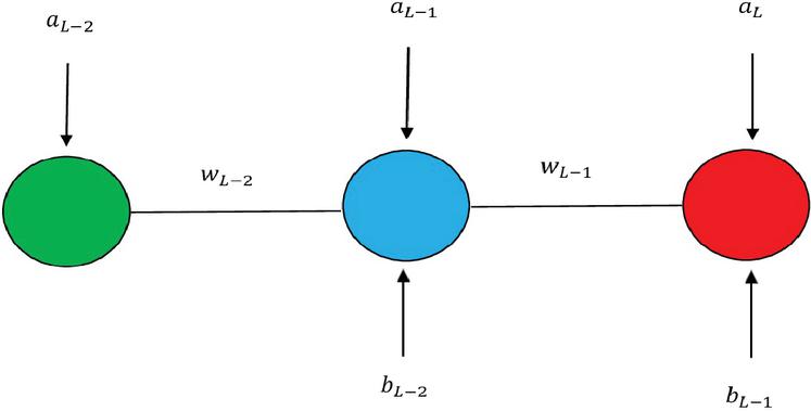
Consider a simple 1-1-1 network (one input (green) - one hidden (blue) – one output (red) layer) as shown in Figure 3. , and are the activation functions of the output, hidden and input neurons respectively. L is the total number of layers in the network. , , and , , are weights and bias between layers respectively. Mean square error can be considered as a cost function and the objective is to minimize the cost function as much as possible [16, 20]. The cost function for an actual value is given as,
| (7) |
Figure 3 1-1-1 network.
• Step2: Gradient calculation with respect to all weights () and bias ()
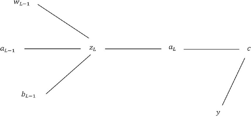
Gradient estimation of the cost function for neurons connecting layer and can be explained with the help of Figure 4. It shows the contribution of different terms to the final layer activation function and cost. The weighted sum of the last layer () can be estimated as the sum of the bias term of the previous layer () and the product of activation and weights between last () and previous () layers [16, 20]. is given as,
| (8) |
Activation of layer can be written as a non-linear function of the weighted sum,
| (9) |
Figure 4 Gradient estimation of L-1.
• Step 3: Weight and bias adjustments based on gradients
Gradient of cost function with respect to weight () can be calculated using chain rule as,
| (10) |
, and are estimated by taking the partial deviates of Equations (7), (8), and (9) respectively [16, 20]. These equations are given as,
| (11) | |
| (12) | |
| (13) |
Substituting Equations (11), (12) and (13) in (10) gives,
| (14) |
Equation (12) can be estimated by taking the derivative of the Sigmoid function in Equation (6) [16, 20]. Change in cost function due to change in bias can be estimated as,
| (15) |
, and can be estimated by taking the partial derivatives of Equations (8), (9), and (7) respectively [16, 20]. These equations are given as,
| (16) | |
| (17) | |
| (18) |
The above equations can be used for weight and bias updation as,
| (19) | |
| (20) |
Change in cost function with respect to the activation function of layer () can be estimated using the chain rule,
| (21) |
, and can be estimated by taking the partial derivatives of Equations (8), (9), and (7) respectively [16, 20].
| (22) | |
| (23) | |
| (24) |
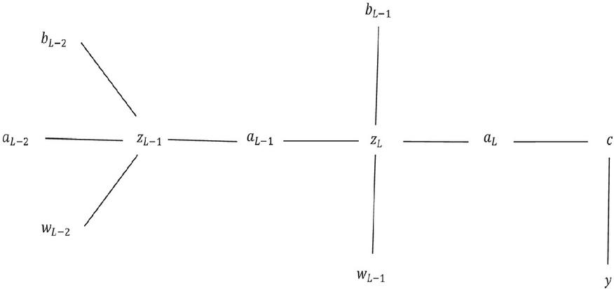
These processes have to be repeated for the layer. Figure 5 shows layer operations. Change in cost function with respect to can be estimated using chain rule as shown below,
| (25) |
Figure 5 Gradient estimation of L-2.
This can be elaborated by substituting the value of as shown below,
| (26) |
and in the above equation can be estimated as,
| (27) | |
| (28) |
Substituting Equations (27) and (28) in (26) gives,
| (29) |
Therefore, the gradient of concerning any weight or any bias can be easily calculated by estimating the derivative of concerning the activation function at each layer. This recursive process is called back-propagation as the gradient propagates in the backward direction. This can be extended to any general network shown in Figure 6. The number of neurons in each layer need not be equal always [16, 20]. The cost function, the weighted sum of layers, and activation of the final layer in a generalized network can be written as,
| (30) | |
| (31) | |
| (32) |
Figure 6 General network.
In the general case, the weighted sum should consider the contributions of all neurons in the previous layer. Superscripts and are used to represent neurons in the previous layer and current layer, respectively [16, 2]. Gradients of the cost function concerning weights and activation function for the generalized network (for L-1 layer, moving back by one layer) can be written as,
| (33) | |
| (34) |
This process can be repeated for layer L-2 (moving back by one more layer). The gradient of the cost function with respect to weight for the generalized network can be written as,
| (35) |
Substituting the value of from Equation (34) in Equation (35) gives,
| (36) |
Equation (36) shows the recursive calculation for the general network. These steps can be repeated for biases of the network. Weights will be updated similarly to the 1-1-1 network case. Forecasts are obtained using finalized weights [16, 2, 20].
2.2 ARIMA Model
Auto-Regressive Integrated Moving Average (ARIMA) is a widely used time series forecasting model. It combines auto-regression and moving average forecasting approaches. Auto-regression uses past time series values called lags. Moving average uses past errors in the time series called error lags. ARIMA blends the best part of both models and its performance is superior to them [1, 11]. Therefore, the ARIMA model is implemented for comparison in the proposed work. ARIMA model for a time series can be defined as,
| (37) | |
| (38) |
where is the random noise occurring at t. and are auto-regression and moving average parameters, respectively. Equations (37) and (38) can be rewritten using Back Operator () [1],
| (39) | |
| (40) |
Equations (39) and (40) can be merged as [1],
| (41) |
Substituting the value of in Equation (41) gives final ARIMA model [1],
| (42) |
Equation (42) is used to obtain very short-term wind power forecasts. Deviation charges are estimated using those forecasts and actual data for comparison.
2.3 Multi Linear Regression
A multi-linear regression model is also implemented for comparison. It is a statistical technique used for time series forecasting. It models a dependent variable using several independent variables [9, 8]. Consider data,
| (43) |
where x,u, and w are independent variables and y is a dependent variable. The Multi-linear regression model is given as,
| (44) |
where , , , and are regression coefficients. These coefficients can be found by the least square method. The model error can be represented as [9],
| (45) |
where and are actual and predicted values, respectively. The objective is to find regression coefficients for minimum error. The least-square minimization is given as [9],
| (46) | |
| (47) |
where N is the number of time instants in an interval. Differentiating with respect to , , and and equating to zero gives,
| (48) | ||
| (49) | ||
| (50) | ||
| (51) | ||
| (52) | ||
| (53) | ||
| (54) | ||
| (55) |
Equation (49) can be rewritten as,
| (56) |
Equation (51) can be rewritten as,
| (57) |
Similarly, we can rewrite Equations (53) and (55). Converting all these equations into matrix form gives [9],
| (58) |
Gauss elimination method is used to find , , and . Equation (44) with estimated parameters is used to obtain very short-term wind power forecasts. Deviation charges are estimated using those forecasts and actual data for comparison.
Proposed ANN and Multilinear regression models are implemented in MATLAB 2021a. ARIMA model is implemented on SAS software. Deviation charge estimation using actual data and forecasts is explained in the next section.
3 Deviation Charge Estimation
The proposed work shows forecasting performance in terms of deviation charge rather than simple error matrices as it represents the financial impacts of forecasting accuracy. This may motivate wind power producers to enhance forecasting accuracy for profit maximization. Positive and negative forecast deviation create almost similar financial impacts, therefore, deviation charges are usually calculated using absolute error and absolute percentage error [24, 18, 5]. Absolute Error (AE) and Absolute Percentage Error (APE) can be calculated using the following equations [24].
| (59) | |
| (60) |
where and are the actual wind power generation and forecast at a particular instant. Deviation charges are estimated for different ranges of absolute percentage error as the impact on the system will be severe for higher deviation. Deviation charges are usually avoided for the APE range of 0 to 15 percent as it results in less impact and also for promoting green energy generation [18, 5]. The deviation charge for the APE range of 15 to 25 % is calculated as,
| (61) |
where is the absolute error above 15 % of APE and K is the Indian Rupee to the dollar conversion factor. Deviation charge for the APE range 25 to 35 % is calculated as [18, 5],
| (62) |
where is the absolute error above 25 % of APE. Deviation charge for the APE above 35 % is calculated as [18, 5],
| (63) |
where is the absolute error above 35% of APE. Deviation charges are estimated at each time instant of a day with a five-minute interval. Deviation charges of proposed ANN and reference models are compared to show the superiority of the proposed model.
4 Results and Discussions
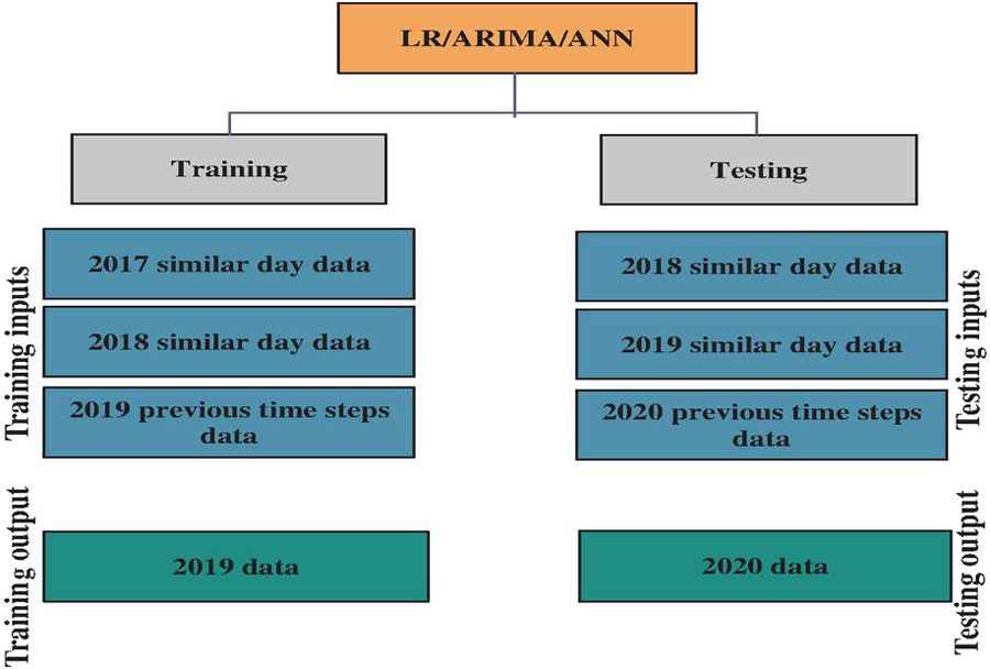
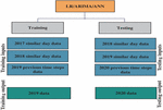
Five-minute-wise wind power generation data from the BPA balancing area (2016 to 2020) is selected for analysis [4]. BPA balancing area has an aggregated wind installed capacity of 3000 MW. Previous time steps and previous year similar day data are used as inputs, because, these data have shown a high auto-correlation. Data selection used for proposed ANN, reference ANN, and ARIMA models are shown in Figure 3. Exogenous factors such as temperature, pressure, and humidity are not considered for forecasting as those data show very low and irregular correlations during empirical analysis. A seasonal analysis is conducted to show the performance throughout the year. Spring, Summer, Fall, and Winter seasons are considered for analysis. Wind power forecasts are obtained using proposed ANN, linear regression, and ARIMA models, and deviation charges are estimated using absolute forecasting errors and absolute percentage forecasting errors.
Figure 7 Data selection.
Figure 8 Wind power (MW) April 3.
Figure 9 Wind power (MW) of July 7.
Figure 10 Wind power (MW) of September 7.
Figure 11 Wind power (MW) of December 10.
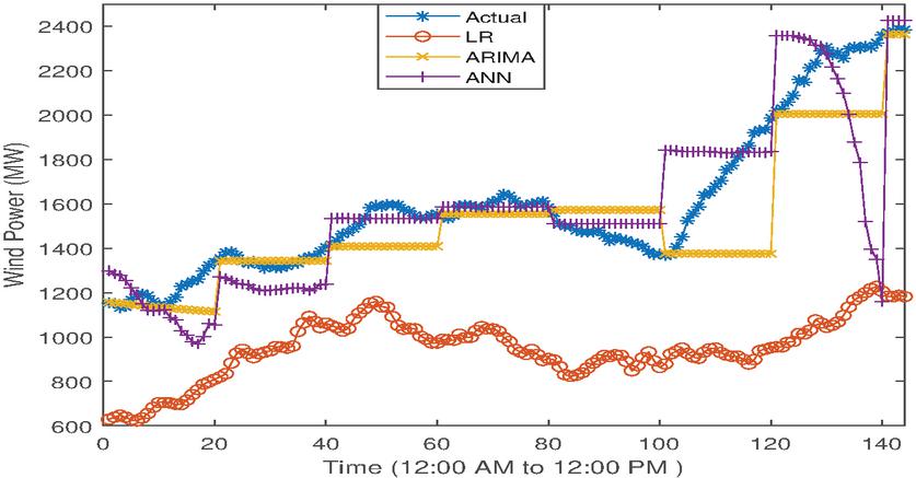
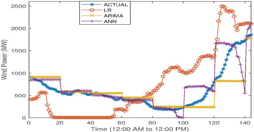
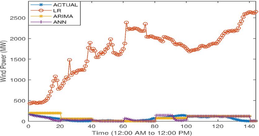
Wind power forecasts of proposed very short-term ANN and reference models for one day in each season are shown in Figures 7, 8, 9, and 10, respectively. April 3, July 7, September 7, and December 10 are taken from the Spring, Summer, Fall, and Winter seasons, respectively. 144 forecasts (five-minute forecasts from 12:00 AM to 12:00 PM) are only shown to avoid the difficulty of including 288 forecasts (whole day) in a single plot. Actual wind power data of the same day was also plotted along with different model forecasts for comparison. These figures show that the proposed ANN model forecasts closely follow the actual values in the Spring, Summer, and Winter seasons compared to linear regression and ANN models. This is due to the proven learning capabilities of back-propagation-based ANN over time series models. ARIMA forecasts are slightly closer than proposed ANN forecasts in the Fall season, however, ANN and ARIMA are closely placed. Linear regression forecasts are far away from actual values in all seasons as linear regression is not suitable for highly non-linear and uncertain data such as wind power.
Figure 12 Absolute percentage errors of April 3.
Figure 13 Absolute percentage errors of July 7.
Figure 14 Absolute percentage errors of September 7.
Figure 15 Absolute percentage error of December 10.
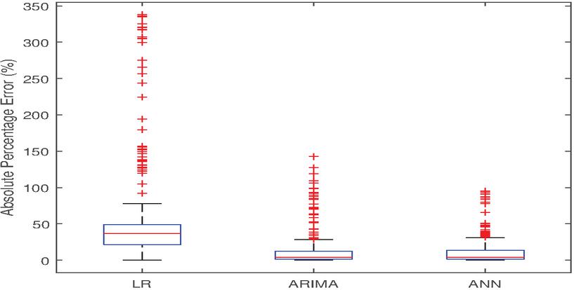
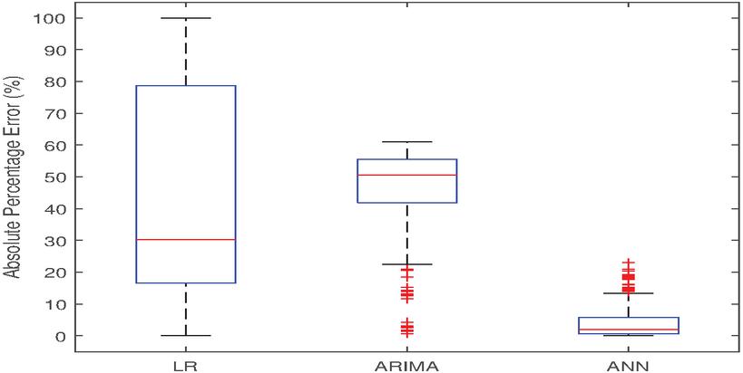
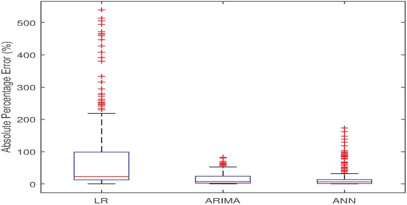
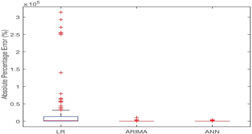
Deviation charge estimation necessitates absolute error and absolute percentage error. These are estimated using forecasts and actual values (Equations (59) and (60)). Absolute percentage errors of one day in each season (April 3, July 7, September 7, and December 10) are shown in Figures 11, 12, 13, and 14 respectively. These box plots show that the absolute percentage errors of the linear regression model are highest in all seasons. The proposed ANN model shows the least absolute percentage error in the Spring, Summer, and Winter seasons and the ARIMA Model shows the least absolute percentage error in the Fall season. However, ARIMA shows only a marginal accuracy improvement in the Fall season over the proposed ANN model. Therefore, the proposed ANN model shows the least absolute percentage error annually. This underlines the improved learning capabilities of the proposed ANN model compared to the time series models (ARIMA and linear regression models).
Figure 16 Deviation charge April 3.
Figure 17 Deviation charge of July 7 .
Figure 18 Deviation charges of September 7.
Figure 19 Deviation charges of December 10.
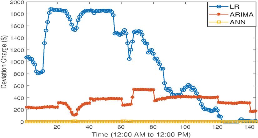
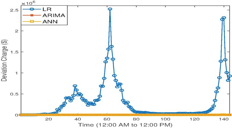
Deviation charges are estimated using Equations (3) to (4) for and taken as zero for . Deviation charges of one day in each season (April 3, July 7, September 7, and December 10) are shown in Figures 15, 16, 17, and 18, respectively. 144 deviation charges (five minutes-wise deviation charges from 12:00 AM to 12:00 PM) are only shown to avoid the difficulty of including 288 deviation charges (whole day) in a single plot. These plots show that wind power producers can reduce deviation charges significantly by using an accurate forecasting model such as the proposed ANN model. The proposed ANN model shows the least deviation charges in the Spring, Summer, and Winter seasons and deviation charges of the Fall season are slightly higher than the ARIMA model. However, the proposed model offers the least deviation charges on an annual basis as it includes all four seasons. The linear regression model shows the highest deviation charges in all seasons. Linear regression deviation charge magnitudes indicate the depth of financial loss that can be incurred due to inaccurate forecasting models.
Table 1 Average deviation charges of different days ($)
| DAYS | LR | ARIMA | ANN |
| APRIL 3 | 430.88 | 40.56 | 24.96 |
| APRIL 5 | 27614.52 | 12.82 | 11.00 |
| APRIL 8 | 6464.83 | 22.31 | 18.11 |
| JULY 1 | 296.85 | 0 | 0 |
| JULY 7 | 508.09 | 228.77 | 0.45 |
| JULY 9 | 529.27 | 946.16 | 0.85 |
| SEP 2 | 4248.24 | 18.77 | 11.16 |
| SEP 6 | 192.26 | 4.00 | 4.65 |
| SEP 7 | 515.90 | 14.92 | 35.23 |
| DEC 6 | 26141.59 | 4.70 | 10.79 |
| DEC 7 | 656945.45 | 26.56 | 18.21 |
| DEC 10 | 505880.59 | 274.96 | 217.02 |
Table 1 shows the average deviation charges ($) of each time instant on different days due to the proposed ANN, ARIMA, and Linear Regression (LR) models. Three days are shown from each season. April 3, April 5, and April 8 are shown from the Spring season. July 1, July 7, and July 9 are shown from the Summer season. September 2, September 6, and September 7 are shown from the Fall season. December 6, December 7, and December 10 are shown from the Winter season. The proposed ANN model shows the least average deviation charges on all days except September 2, September 6, September 7, and December 6. The first three days belong to the Fall season and the last day belongs to the Winter season, where deviation charges of the proposed ANN model are higher than the ARIMA model. Moving average estimation in the Fall season and the first day of Winter has shown superiority compared to ANN learning as data show moving patterns and results in the least deviation charges for ARIMA models. Table 2 shows the average deviation charges of different seasons due to the proposed ANN and reference models (LR and ARIMA). There are 45494.16%/40%, 13.55%/90979.06%, and 38817.36%/24.4% average deviation charge reduction can be observed from LR to ARIMA/ARIMA to proposed ANN in Spring, Summer, and Winter season respectively. The fall season shows 9612.69% and 35.42% average deviation charge reduction from LR to ANN and ANN to ARIMA respectively.
Table 2 Average deviation charges of different seasons ($)
| SEASONS | LR | ARIMA | ANN |
| SPRING | 11,503.41 | 25.23 | 18.023 |
| SUMMER | 444.74 | 391.64 | 0.43 |
| FALL | 1,652.13 | 12.56 | 17.01 |
| WINTER | 396,322.54 | 102.073 | 82.00 |
Table 3 Total deviation charges of different days ($)
| DAYS | LR | ARIMA | ANN |
| APRIL 3 | 124093.59 | 11682.36 | 7189.32 |
| APRIL 5 | 7952982.27 | 3693.01 | 3169.03 |
| APRIL 8 | 1861872.04 | 6427.07 | 5216.75 |
| JULY 1 | 85493.74 | 0 | 0 |
| JULY 9 | 152430.89 | 272495.55 | 245.52 |
| JULY 7 | 146332.12 | 65886.44 | 130.69 |
| SEP 2 | 1223493.75 | 5406.94 | 3214.35 |
| SEP 6 | 192.26 | 1152.26 | 1341.68 |
| SEP 7 | 515.90 | 4299.09 | 10146.42 |
| DEC 6 | 7528780.31 | 1354.57 | 3109.97 |
| DEC 7 | 189200291.7 | 7651.80 | 5245.16 |
| DEC 10 | 145693611 | 79189.59 | 62502.96 |
Table 3 shows the total deviation charges (sum of 288 time steps) of different days due to the proposed ANN, ARIMA, and LR models. It can be observed that total deviation charges also follow the same pattern. The proposed ANN model shows the least total deviation charges in all days of Spring, Summer, and two days of Winter seasons. ARIMA model shows the least total deviation charges on all days of the Fall season and one day of the winter season. There are 454864.40%/39.98% and 13.55%/89844.97% and 388152.11%/24.46% total deviation charge reduction can be observed from LR to ARIMA/ARIMA to proposed ANN in Spring, Summer and Winter season respectively. The fall season shows 8226.51% and 35.40% total deviation charge reduction from LR to ANN and ANN to ARIMA respectively. ARIMA model shows an annual total deviation charge reduction of 76977.58% from linear regression and the proposed ANN model shows an annual deviation charge reduction of 352.39% from ARIMA. This shows that the proposed ANN model has a strong potential to reduce deviation charges.
5 Conclusions
Very high penetration of uncertain and variable wind generation results in various system operational challenges such as frequent system imbalances. This leads to the deployment of additional balancing services such as flexible ramp products and increased total operation costs. Increased operational costs are transferred to wind power producers as deviation charges. This reduces the profit of wind power producers. Deviation charges are estimated from the magnitude of deviation of actual generation from forecasts. Therefore, deviation charges can be reduced by improving wind power forecasting accuracy. Also, existing wind power forecasting studies show performance in terms of error matrices. These error matrices do not show any implication about the financial impact of forecasting error. Expressing forecasting performance in financial terms such as deviation charges motivates wind power producers to reduce forecasting errors.
In this context, this paper proposes an ANN-based very short-term wind power forecasting model to reduce deviation charges. The seasonal analysis is conducted to show performance throughout the year. An analysis is conducted on the data collected from the BPA balancing area. The proposed model performance is compared with linear regression and ARIMA models. The comparison shows that the proposed ANN model gives the least deviation charges in the Spring, Summer, and Winter seasons and the Fall season deviation charges are higher than the ARIMA model. Annually, proposed ANN models outperform all reference models. This shows that the proposed very short-term ANN model has a strong potential to reduce deviation charges. However, deviation charges can be further reduced by more sophisticated machine learning models such as deep learning models. This can be done as future work.
Data Availability Statement
The data sets generated during and/or analyzed during the current study are available in [27].
References
[1] R. Adhikari and R. K. Agrawal. An introductory study on time series modeling and forecasting. book, arXiv preprint arXiv:1302.6613, 2013.
[2] I. Argatov. Artificial neural networks (anns) as a novel modeling technique in tribology. Frontiers in Mechanical Engineering, 2019. 30.
[3] P. S. Bharadwaj, R. K., and H. R. Sridevi. Dsm in forecasting and scheduling for improving integration of renewable energy generation to the grid. In Proc., International Conference on Recent Trends on Electronics, Information, Communication & Technology (RTEICT), pages 649–654, 2019.
[4] Bonneville Power Administration. Balancing area wind generation and load data, Accessed date: 15/12/2021. 2021.
[5] CEA. Framework on forecasting, scheduling and imbalance handling for variable renewable energy sources (wind and solar). Technical Report, CEA, Government of India, 2016. 1–77.
[6] Y. Dong, L. Zhang, Z. Liu, and J. Wang. Integrated forecasting method for wind energy management: A case study in china. Processes, 2020. 8(1):35.
[7] A. Gupta, K. C. Sharma, A. Vijayvargia, and R. Bhakar. Very short term wind power prediction using hybrid univariate arima-garch model. In Proc., International Conference on Power Systems (ICPS), pages 1–6, 2019.
[8] A. Hosseinzadeh, M. Baziar, H. Alidadi, J. L. Zhou, A. Altaee, A. A. Najafpoor, and S. Jafarpour. Application of artificial neural network and multiple linear regression in modeling nutrient recovery in vermicompost under different conditions. Bioresource Technology, 2020. 303:122926.
[9] J. D. Jobson. Multiple linear regression. Springer Texts in Statistics. Springer, New York, NY, 1991.
[10] K. Kalaiselvi, K. Velusamy, and C. Gomathi. Financial prediction using back propagation neural networks with opposition based learning. Journal of Physics: Conference Series, 2018. 1142(1):012008.
[11] F. Kaytez. A hybrid approach based on autoregressive integrated moving average and least-square support vector machine for long-term forecasting of net electricity consumption. Energy, 2020. 197:117200.
[12] Yan Liang, Li Zhi, and Yu Haiwei. Medium-term load forecasting method with improved deep belief network for renewable energy. Distributed Generation & Alternative Energy Journal, pages 485–500, 2022.
[13] C. Lins, L. E. Williamson, S. Leitner, and S. Teske. The first decade: 2004–2014:10 years of renewable energy progress. Renewable Energy Policy Network for the 21st Century, 2014.
[14] Y. V. Makarov, C. Loutan, J. Ma, and P. De Mello. Operational impacts of windgeneration on california power systems. IEEE Transactions on Power Systems, 2009. 24(2):1039–1050.
[15] J. Matevosyan and L. Soder. Minimization of imbalance cost trading wind power on the short-term power market. IEEE Transactions on Power Systems, 2006. 21(3):1396–1404.
[16] R. Mutihac. Mathematical modeling of artificial neural networks. In Encyclopedia of Artificial Intelligence, IGI Global, 2009. 1056–1063.
[17] Xiumin Niu and Xufeng Luo. Policies and economic efficiency for distributed photovoltaic and energy storage industry. Distributed Generation & Alternative Energy Journal, pages 1197–1222, 2023.
[18] Forum of Regulators. Dsm in forecasting and scheduling for improving integration of renewable energy generation to the grid. Technical Report, CEA, Government of India, 2015. 1–33.
[19] X. Peng, D. Deng, J. Wen, L. Xiong, S. Feng, and B. Wang. Very short term wind power forecasting approach based on numerical weather prediction and error correction method. In Proc., China International Conference on Electricity Distribution (CICED), pages 1–4, 2016.
[20] X. Shen, Y. Zheng, and R. Zhang. A hybrid forecasting model for the velocity of hybrid robotic fish based on back-propagation neural network with genetic algorithm optimization. IEEE Access, 2020. 8:111731–111741.
[21] J. Shi, Z. Ding, W. J. Lee, Y. Yang, Y. Liu, , and M. Zhang. Hybrid forecasting model for very-short term wind power forecasting based on grey relational analysis and wind speed distribution features. IEEE Transactions on Smart Grid, 2013. 5(1):521–526.
[22] S. Sreekumar, K. C. Sharma, and R. Bhakar. Grey system theory based net load forecasting for high renewable penetrated power systems. Technology and Economics of Smart Grids and Sustainable Energy, 2020. 1–14.
[23] S. Sreekumar, K. C. Sharma, and R. Bhakar. Multi-interval solar ramp product to enhance power system flexibility. IEEE Systems Journal, 2021. 15(1):170–179.
[24] S. Sreekumar, K. C. Sharma, R. Bhakar, S. Chawda, F. Teotia, , and V. Prakash. Deviation charge reduction of aggregated wind power generation using intelligently tuned support vector regression. In Proc., International Conference on Power Systems (ICPS), pages 1–6, Jaipur, Rajasthan, 2019. IEEE.
[25] L. Tan, J. Han, and H. Zhang. Ultra-short-term wind power prediction by salp swarm algorithm-based optimizing extreme learning machine. IEEE Access, 2020. 8:44470–44484.
[26] Y. Tao, Y. Zhang, B. Chen, and J. Shi. A combined approach for very short term wind power probability forecast. In Proc., International Conference on Power System Technology (POWERCON), pages 874–880, 2018.
[27] Zhang Yiming and Cheng Li. Short-term wind power prediction method based on uav patrol and deep confidence network. Distributed Generation & Alternative Energy Journal, pages 1739–1754, 2022.
[28] H. Zhang, Y. Liu, J. Yan, S. Han, L. Li, and Q. Long. Improved deep mixture density network for regional wind power probabilistic forecasting. IEEE Transactions on Power Systems, 2020. 35(4):2549–2560.
[29] H. Zhang, J. Yan, Y. Liu, Y. Gao, S. Han, and L. Li. Multi-source and temporal attention network for probabilistic wind power prediction. IEEE Transactions on Sustainable Energy, 2021. 12(4):2205–2218.
[30] B. Zhou, X. Ma, Y. Luo, and D. Yang. Wind power prediction based on lstm networks and nonparametric kernel density estimation. IEEE Access, 2019. 7:165279–165292.
Biographies

Sandhya Kumari received the B.Tech. degree in electrical and electronics engineering (EEE) from Government Engineering College, Bhuj, Gujarat (GTU, Gujarat India), in 2019, and the M.Tech (Power Systems) degree from DIT University in 2022. Her research interest includes load forecasting and renewable generation forecasting.

Sreenu Sreekumar received the B.Tech. degree in electrical and electronics engineering (EEE) from Government Engineering College, Idukki, Kerala (Mahatma Gandhi University, Kerala, India), in 2012, and the M.Tech (Power Systems) and Ph.D. (Electrical Engineering) degree from Malaviya National Institute of Technology Jaipur, Jaipur, India, in 2015 and 2020 respectively. He received the prestigious POSOCO Power System Award 2016 (National level) for the best M-tech level power system research. He was a Post-Doctoral Research Fellow at NIT Trichy. Currently, he works as an Assistant Professor in the electrical engineering department at NIT Silchar, Assam. He has 35 international publications (15 Journal Papers, 19 conference papers, and one book). His research interest includes power system flexibility enhancement, load forecasting, renewable generation forecasting, mathematical modelling of motors for electric vehicles, and Net Zero targets.

Sonika Singh The alumnus of Mumbai University, received her B.E. in Electronics & Telecommunication Engineering from Mumbai University in 1998 and M.Tech. in Digital Communication from U.P. Technical University Lucknow, in 2007. She has also done PGDBM in Marketing Management. She did her Ph.D. in 2012 in Electronics and Communication Engineering from Uttrakhand Technical University.
Holding her Ph.D. in Electronics and Communication Engineering, she is mentoring the young minds at DIT University to leverage the most in this field. Dr. Sonika authored a book on ‘Solid State Devices & Circuit’ in 2004 and proudly owns the publication of more than thirty papers in Conference Proceedings and International Journals.
She proudly walks along an exceptional experience of more than twenty-one years, rendering additional administrative responsibilities at DIT University. She acts as a significant member of several university-centric committees while chairing the Board of Studies for the School of Architecture, MCA, and Physics as an External Member. Her research interests include Mobile Satellite Systems, Photonics, and Channel modelling in Wireless Communication Systems, Dr. Sonika has guided one Ph.D. in EECE Department. She is also the Founder and Chairperson of ICEIT (Institution of Communication Engineers and Information Technologists). She is also mentoring NPTEL Online Certification Courses and has recently been awarded a Certificate of Recognition by The Academic Council of uLektz as one of India’s Top 50 Women Leaders in the Education Industry for the year 2020.

D. P. Kothari received his B.E. (Electrical), M.E. (Power Systems), and doctoral degree in Electrical Engineering from the Birla Institute of Technology & Science, Pilani. His activities include Optimal Hydro-thermal Scheduling, Unit Commitment, Maintenance Scheduling, Energy Conservation (loss minimization and voltage control), and Power Quality and Energy Systems Planning and Modelling. He has guided 16 Ph.D. scholars and has contributed extensively in these areas as evidenced by the 335 research papers published by him in various national and international journals. Prof. Kothari has also authored 12 books on Power Systems. He was a visiting professor at the Royal Melbourne Institute of Technology, Melbourne, Australia in 1982 and 1989. He was an NSF Fellow at Purdue University in 1992. He has visited and delivered several invited talks, and keynote addresses at both national and international conferences on Electric Energy Systems. He has received several best paper awards and gold medals for his work. He has been Principal (1997–98), Visvesvaryaya Regional Engineering College, Nagpur.
Distributed Generation & Alternative Energy Journal, Vol. 39_1, 27–56.
doi: 10.13052/dgaej2156-3306.3912
© 2023 River Publishers

