The Optimal Placement of Electric Vehicle Fast Charging Stations in the Electrical Distribution System with Randomly Placed Solar Power Distributed Generations
Fareed Ahmad1,*, Atif Iqbal2, Imtiaz Ashraf1, Mousa Marzband3 and Irfan Khan4
1Department of Electrical Engineering, Aligarh Muslim University, Uttar Pradesh, India
2Department of Electrical Engineering, Qatar University, Doha, Qatar
3Department: Mathematics, Physics, and Electrical Engineering, Northumbria University, UK
4Clean and Resilient Energy Systems (CARES) Lab, Texas A&M University, Galveston, USA
E-mail: fareed903@gmail.com; atif.iqbal@qu.edu.qa; iashraf@rediffmail.com; mousa.marzband@northumbria.ac.uk; irfankhan@tamu.edu
*Corresponding Author
Received 11 January 2022; Accepted 23 February 2022; Publication 29 April 2022
Abstract
The growing use of electric vehicles (EVs) in today’s transport sector is gradually reducing the use of petroleum-based vehicles. However, as EV penetration grows, the EV’s demand influences distribution network parameters such as power loss, voltage profile. Therefore, an improved bald eagle search (IBES) algorithm is suggested for the optimal placement of FCSs into the distribution network with high penetration of randomly distributed solar power generation (SPDG). This study suggests a two-stage approach for placing FCSs. The charging station investor decision index (CSIDI) was introduced in the first stage, taking into account the land cost index (LCI) and the electric vehicle population index (EVPI). The CSIDI was developed to decrease land costs while increasing EV population for FCS installation. In the next one, an optimization problem is constructed to minimize total active power loss while taking distribution system operator (DSO) constraints into consideration. The IEEE-34 bus distribution system is used as the proposed network. The simulation is carried out in MATLAB to integrate the EVCSs in three cases in the distribution network with SPDGs randomly placed. Therefore, The IBES found the best optimal positions with a power loss of 198.43 kW. When compared to the PSO technique, the IBES technique has a reduced average power loss of 2.02%.
Keywords: Charging stations, electric vehicle population, land cost, improved bald eagle search algorithm, optimal placement.
List of Abbreviations
| CS | Charging Station |
| LCI | Land Cost Index |
| EVPI | Electric Vehicle Population Index |
| CSIDI | Charging Station Investor Decision Index |
| DSO | Distribution System Operator |
| EV | Electric Vehicle |
| FCS | Fast Charging Station |
| PSO | Particle Swarm Optimization |
| GWO | Grey Wolf Optimization |
| BFS | Backward Forward Sweep |
| SPDG | Solar Power Distributed Generation |
| BES | Bald Eagle Search |
| IBES | Improved Bald Eagle Search |
1 Introduction
Electric vehicles (EVs) are gaining popularity among government organizations and the automotive industry due to significant reductions in CO emissions and maintenance costs when compared to the most populous internal combustion vehicles [1]. Furthermore, according to a study, the fossil fuel reserves will be depleted in this century, with oil lasting 51 years, natural gas lasting 53 years, and coal lasting 114 years [2]. Moreover, the researchers examined data to determine that the development of EVs could reduce CO emissions by 28% by 2030 [3]. As a result, the global EV population is growing, posing new challenges for DSO. In addition, new business opportunities are developing, such as service providers for EV consumers, load demand management, and ancillary services. As a result, excessive electrical power demand may affect distribution system parameters such as bus voltages, power loss, reliability, harmonic distortion, voltage imbalance and power quality [4]. Furthermore, the rapidly expanding EV population necessitates the development of well-developed charging infrastructure. Charging stations (CSs) are classified as slow, medium, fast and ultra-fast based on their charging time and power rating [5].
FCSs are an appropriate choice for charging EV batteries in 20–30 minutes [6]. As a result, installing FCSs is a beneficial option for EV customers; nevertheless, installing FCSs has a negative influence on the distribution system [7]. Furthermore, the proper placement of FCS can reduce the burden on the distribution system [8]. Furthermore, the number of FCSs and their locations are critical problems for DSOs, charging station investors and EV consumers. As a result, the number of FCSs and the appropriate location of FCSs have become more interesting study topics in the previous decade. Furthermore, most studies have published their findings on FCS placement by including DSO parameters such as bus voltage, power loss, and reliability [9]. On the other hand, the placement of FCSs has taken into account the investment cost as well as the EV user’s approach. The authors are motivated by the current literature to place the FCS using the DSO approach, the EV users approach, and the FCS investor approach.
1.1 Literature Review
Most of the researchers have worked for the placement of slow or medium charging stations whereas, some authors have discussed the optimal location for FCS. In addition, very little research has been published on the integration of medium and fast charging together. In [10], optimal siting and sizing of CS optimization problem is formulated for obtaining the optimal results by considering investment cost, connection cost, active power losses cost and demand response, which is solved by PSO algorithm. The authors created a multi-objective mixed integer non-linear problem (MINLP) in [11] including FCS development costs, EV specific energy consumption costs, electrical network power loss costs, DGs costs, and voltage variation costs. In addition, the simultaneous allocation of EV parking lots and the distributed renewable resources have been placed at the optimal location through the ant colony optimization (ACO) algorithm [12]. Eventually, a multi-objective problem has formulated considering the minimization of power loss and maximizing the EV population for the optimal CS location which was gained by the grey wolf optimization (GWO) technique [13].
In [14], The authors employed a hybrid Chicken Swarm Optimization and Teaching Learning Based Optimization method to reduce the investment cost for establishing the charging station, as well as a voltage deviation, reliability, and power loss (VRP) index to improve distribution system characteristics. Furthermore, in [15], the same authors have published a literature review on optimal location and sizing of CSs, the impact on distribution systems, and techniques for solving the corresponding problem.
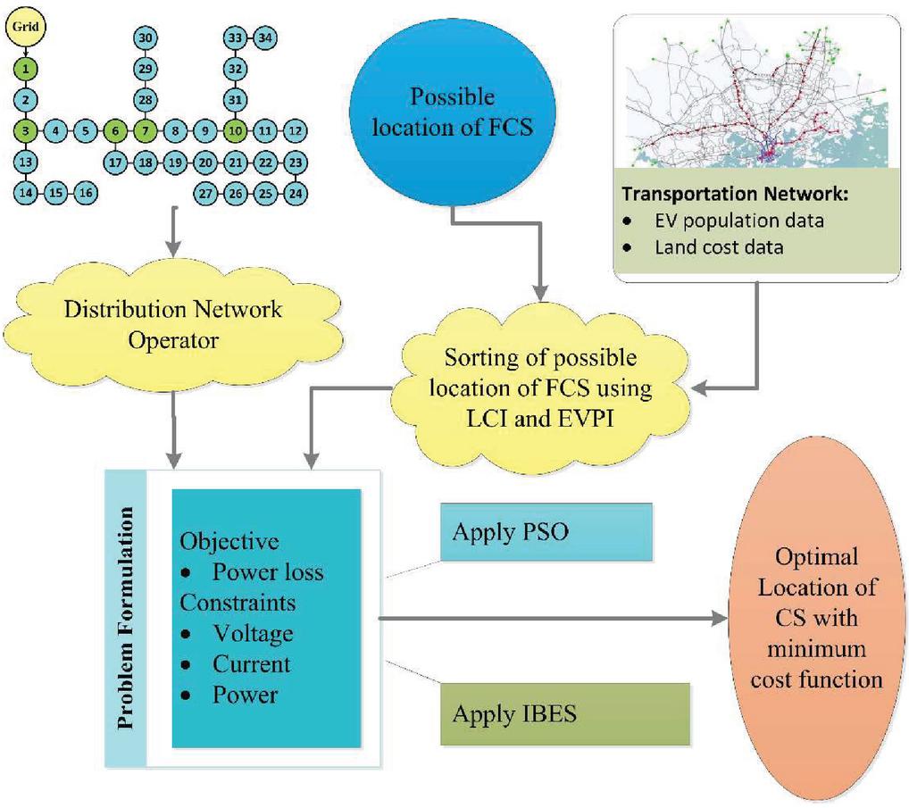
Figure 1 The framework of the proposed problem.
Furthermore, the authors in [16], proposed a capacitated-flow refueling location model (CFRLM) and formulated an optimization problem that included investment cost, penalty for unsatisfied charging demands, and power distribution network cost, which is solved by branch and bound (B&B) technique. Moreover, the stability and power loss minimization is the objective function of the optimization problem which is solved by the adaptive particle swarm optimization (APSO) algorithm [17]. Similarly, in [6], the power loss and voltage deviation have been selected as objective functions for CS placement with the integration of PV generation while formulated problem solved by PSO method. Furthermore, a mixed-integer programming model has been established to express the problem of optimizing total plug-in EV populations in the network, and the GA has been utilized to solve the suggested problem [18]. In [19], the authors have suggested the multi-objective approach for the placement of CSs and DGs with V2G strategy, whereas an improved harmony PSO algorithm has obtained the optimal results of the proposed problem. Moreover, the authors in [20], have suggested the fuzzy grasshopper optimization algorithm for optimal placement of CSs, DGs, and shunt capacitors. Furthermore, in [9] authors have obtained the optimal location of CS by minimizing the development cost of CS, power loss, and maximizing the voltage quality, and formulated problem is solved by a balanced mayfly algorithm.
1.2 Objectives and Contribution of the Proposed Work
The objective of this research is to determine the optimal locations for FCSs while reducing investment costs and increasing profit from installation, as well as to optimize distribution system parameters. Therefore, for the modeling of the optimization problem, land cost, EV population, and power loss of distribution system are considered as the objective for the placement of charging stations. All the existing structures aim to achieve the optimal location of the CS considering various objective functions. However, to the best of the authors’ knowledge, no such method has considered the land cost and EV population in the optimization problem. In this paper, a novel approach for the location of FCSs is proposed considering the land cost, EV population, and power loss cost. This synchronic approach significantly enhances the productivity of smart distribution networks in terms of reaching the best degree of loss reduction by incorporating both the charging station investor’s decision factor and distribution network constraints.
The optimal location of FCSs is identified in two stages. CSIDI is optimized in the first phase for sorting the possible locations for FCSs that increase EV population while minimizing land cost. Furthermore, power loss is reduced for the next phase to get the optimal locations. The majority of the presented study has determined the optimal location of CS by taking installation costs, quality enhancement parameters of distribution systems, and their combination into account. For the placement of FCSs in this study, installation cost, quality enhancement component of the distribution system, and profit were all taken into account.
The main contribution of this paper is expressed as:
• A two-stage novel optimization problem is developed to maximize the EV population while reducing investment costs and power loss costs for the FCSs deployment.
• In the first step, the charging station investor decision index (CSIDI) is developed to reduce the optimization algorithm’s search space. Furthermore, the LCI and EVPI are established to optimize the value of land cost and EV population for the investor to receive more return with less capital for FCS installation.
• In the second phase, a single objective optimization problem with power loss cost as the objective function is created to identify the optimal positions from the first stage identified locations. Furthermore, the Improved Bald Eagle Search algorithm has been proposed for the optimal solutions of the specified optimization problem to optimize the FCSs position to increase their performance in terms of power loss, and the obtained results were compared with the PSO algorithm.
• The integration of EV charging stations with randomly placed solar power distribution generation (SPDG) for distribution network is presented realistically and thoroughly, taking into account electrical and geographic limits.
1.3 Organization of the Paper
The remainder of this work is structured as follows: Section 2 presents the problem formulation for optimal FCS placement. Section 3 illustrates the optimization technique for achieving the optimal solution. Section 4 further explains the results of the presented problem. Section 5 brings the paper to a conclusion.
2 Problem Formulation
Figure 1 is suggested the problem framework for optimal FCS location, therefore the EV charging station investor decision index (CSIDI) is framed by including the land cost for FCS installation and EVs population at each bus. Furthermore, the objective function under the distribution system operator approach is suggested with some distribution constraints. Afterward, the price of land in the cities is very high and sometimes changes within a city with very high differences. Therefore, the FCS investors first ruminate the land cost for the placement of FCS. On the other side, the FCS location should be accessible by the EV users, therefore the FCS investors investigate the EV population at all possible FCS locations to maximize the profit. Eventually, the optimization problem is created to minimize the power loss of the distribution system with network constraints for the optimal FCS location. In addition, first, calculate the number of FCS in the proposed area with the IEEE-34 bus system to obtain the optimal location.
2.1 Formulation of Charging Station Investor Decision Index
The number of FCSs in the intended region was calculated by looking at the overall EV population in the area, battery capacity, load factor, and charging time, which is expressed in (1) [21]. As a result, the number of FCS (N) is illustrated.
| (1) |
Where p is the mean power of EVs, N is the number of EVs to be charged per day, ch_time is the charging time, st is the charger service time, C is the capacity of fast charger, q is charging efficiency, lf is the load factor of the charger.
Table 1 IEEE34 Bus Load data, line data, and EV population
| Bus | Load | Load | EVs | From | To | Resistance | Reactance |
| No. | (kW) | (kVAR) | Population | Bus | Bus | (ohm) | (ohm) |
| 1 | 0 | 0 | 0 | 1 | 2 | 0.117 | 0.048 |
| 2 | 230 | 142.5 | 10 | 2 | 3 | 0.1072 | 0.044 |
| 3 | 0 | 0 | 100 | 3 | 4 | 0.1644 | 0.0456 |
| 4 | 230 | 142.5 | 20 | 4 | 5 | 0.1495 | 0.0415 |
| 5 | 230 | 142.5 | 30 | 5 | 6 | 0.1495 | 0.0415 |
| 6 | 0 | 0 | 30 | 6 | 7 | 0.3144 | 0.054 |
| 7 | 0 | 0 | 40 | 7 | 8 | 0.2096 | 0.036 |
| 8 | 230 | 142.5 | 40 | 8 | 9 | 0.3144 | 0.054 |
| 9 | 230 | 142.5 | 50 | 9 | 10 | 0.2096 | 0.036 |
| 10 | 0 | 0 | 50 | 10 | 11 | 0.131 | 0.0225 |
| 11 | 230 | 142.5 | 50 | 11 | 12 | 0.1048 | 0.018 |
| 12 | 137 | 84 | 50 | 3 | 13 | 0.1572 | 0.027 |
| 13 | 72 | 45 | 60 | 13 | 14 | 0.2096 | 0.036 |
| 14 | 72 | 45 | 80 | 14 | 15 | 0.1048 | 0.018 |
| 15 | 72 | 45 | 100 | 15 | 16 | 0.0524 | 0.009 |
| 16 | 13.5 | 7.5 | 120 | 6 | 17 | 0.1794 | 0.0498 |
| 17 | 230 | 142.5 | 150 | 17 | 18 | 0.1644 | 0.0456 |
| 18 | 230 | 142.5 | 170 | 18 | 19 | 0.2079 | 0.0473 |
| 19 | 230 | 142.5 | 200 | 19 | 20 | 0.189 | 0.043 |
| 20 | 230 | 142.5 | 30 | 20 | 21 | 0.189 | 0.043 |
| 21 | 230 | 142.5 | 20 | 21 | 22 | 0.262 | 0.045 |
| 22 | 230 | 142.5 | 20 | 22 | 23 | 0.262 | 0.045 |
| 23 | 230 | 142.5 | 10 | 23 | 24 | 0.3144 | 0.054 |
| 24 | 230 | 142.5 | 10 | 24 | 25 | 0.2096 | 0.036 |
| 25 | 230 | 142.5 | 10 | 25 | 26 | 0.131 | 0.0225 |
| 26 | 230 | 142.5 | 10 | 26 | 27 | 0.1048 | 0.018 |
| 27 | 137 | 85 | 30 | 7 | 28 | 0.1572 | 0.027 |
| 28 | 75 | 48 | 30 | 28 | 29 | 0.1572 | 0.027 |
| 29 | 75 | 48 | 20 | 29 | 30 | 0.1572 | 0.027 |
| 30 | 75 | 48 | 20 | 10 | 31 | 0.1572 | 0.027 |
| 31 | 57 | 34.5 | 20 | 31 | 32 | 0.2096 | 0.036 |
| 32 | 57 | 34.5 | 20 | 32 | 33 | 0.1572 | 0.027 |
| 33 | 57 | 34.5 | 10 | 33 | 34 | 0.1048 | 0.018 |
| 34 | 57 | 34.5 | 10 | 1 | 2 | 0.117 | 0.048 |
2.2 Formulation of Charging Station Investor Decision Index
2.2.1 Land cost index
The land prices in cities are quite high, and they vary greatly within the city. As a result, FCS investors first analyze the land costs of each possible FCS location. Furthermore, for the probable position of FCS, each bus of the proposed IEEE-34 distribution system should be evaluated. In addition, the land cost index is proposed to include the land cost in problem design. As a result, the load cost data on the buses, branch line data, and EV population on each bus are stated in Table 1 for the IEEE-34 bus system, and a single line diagram of the IEEE-34 bus system is represented in Figure 2. Furthermore, the normalized LCI is represented in (2) for each bus, which is calculated by dividing the land cost of each bus by the maximum land cost of the buses. Therefore, the LCI lay between 0 and 1 according to the land cost on buses.
| (2) |
where, is the land cost at th bus, Nb is the total buses in the distribution system.
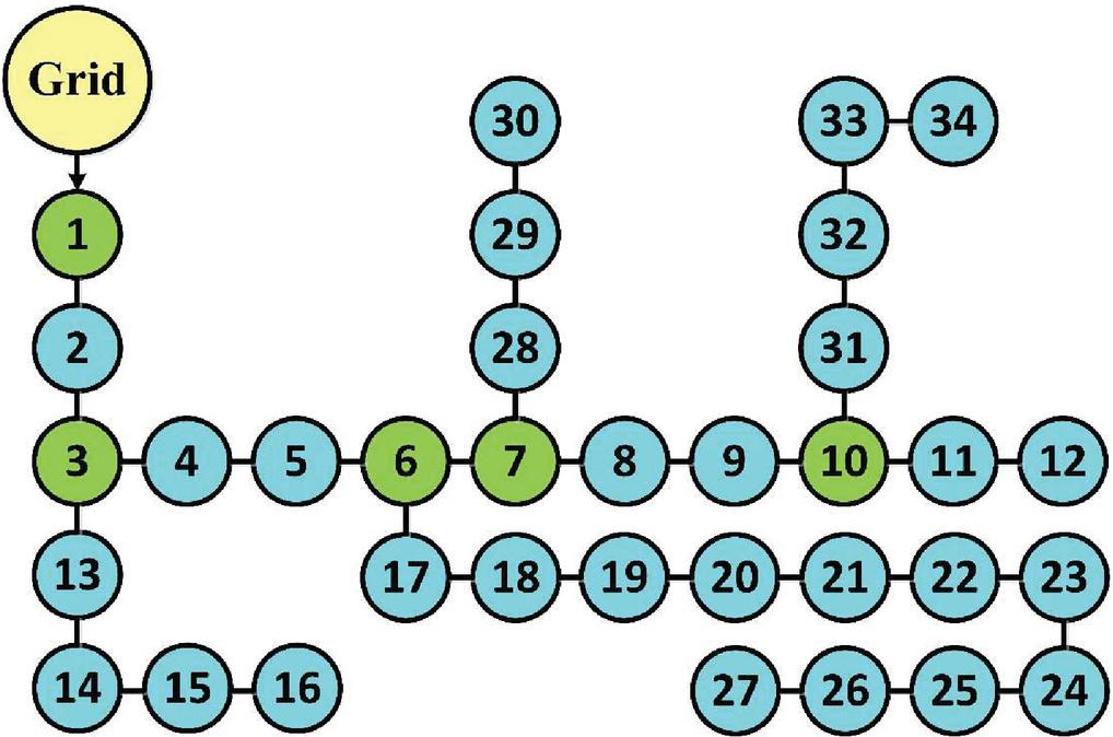
Figure 2 Presentation of an IEEE-34 bus system.
2.2.2 Electric vehicle population index
Furthermore, the number of EVs charged at the FCS will decide the investor profit. In other words, the profit is determined by the number of EVs on the bus. Furthermore, for each bus, an electric vehicle population index (EVPI) is produced, which is used to rank the buses with the highest EV population. Furthermore, the normalized EVPI at each bus is calculated, which is stated in (3) as the EVs at each bus divided by the maximum EVs of the buses.
| (3) |
where, is the EV population at th bus.
Finally, the charging station investor decision index (CSIDI) is represented in (4), which is the combination of the normalized LCI and EVPI for each bus.
| (4) |
where and are the positive coefficients that are used to change the priorities in decision making between land cost and EV population. In addition, and both have 0.5 values for equal weightage for the land cost and EV population.
According to the proposed CSIDI, the investor chooses to install the FCS in the bus, which meets the following conditions. (1) cheaper land cost attracts investors for FCS installation, and (2) large EV population at buses is also chosen by investors for maximum profit.
2.3 Objective Function
As stated in the CSIDI formulation, the possible location for FCS has been narrowed down due to land cost and EV population sorting. In the second step, the optimization problem is phrased further by employing power loss as an objective function with certain inequality constraints. As a result, the objective function for minimizing distribution network power loss is depicted in (5).
| (5) |
where, is the power loss for th branch in the distribution system, br is the total number of branches in the distribution system.
Constraints:
Voltage constraint: The magnitude of the voltage at each node must be kept within acceptable limits, which is expressed in (6).
| (6) |
where and are the minimum and maximum voltage limits of buses, is the voltage of th bus.
Current constraint in branches: The capacity of the distribution line must not be exceeded (7).
| (7) |
where and is the maximum current limits of buses, is the current flow in th line.
Reactive power constraints: to maintain the reactive power of each bus within limitations, a reactive power restriction has been created (8).
| (8) |
where and are the minimum and maximum reactive power limits of buses, is the reactive power at th bus.
2.4 Solar Power Distributed Generation
By 2040, global energy demand will increase by one-third, owing mostly to increased transportation use in China, India, and other Asian countries [22]. Solar power distributed generation (SPDG) is a fast-growing source of renewable energy for the grid. As a result, there have already been a huge number of articles on solar efficiency and solar converters. Furthermore, the integration of FCSs into the grid has resulted in a mismatch between power consumption and electricity output. As a result, the SPDG position was generated at random on the distribution network buses, as shown in Table 2. Furthermore, including SPDG into the distribution network world minimizes grid stress induced by EV load. The SPDG locations are eventually determined at random because the authors only recommended the FCS placement in this article.
Table 2 Placement of SPDGs with capacity
| Types of DGs | Location at Bus | Capacity (kW) |
| SPDG1 | 6 | 250 |
| SPDG2 | 11 | 250 |
| SPDG3 | 22 | 500 |
3 Solution Technique
To get the optimum solution or the unconstrained maxima and minima of continuous and differentiable functions, classical optimization techniques can be applied. Furthermore, because they need objective functions that are not continuous and/or differentiable, classical approaches have limited practical use. As a result, advanced optimization techniques are employed to achieve the best solution to the defined optimization problem. The results of unimodal function from F1–F7 are represented in Table 3 for proposed techniques. Further, the results of the multimodal benchmark from F8–F13 are given in Table 4. Moreover, the results of composite benchmark functions from F14–F23 are obtained in Table 5 for the suggested algorithm. For the benchmark function, the IBES algorithm got the best results, therefore the authors in this paper proposed an IBES algorithm for the optimal location of the charging station.
Table 3 Parameters
| Parameters Name | Value | Unit |
| Number of EVs (N) | 1620 | – |
| Charging time (Ch_time) | 0.33 | hours |
| Capacity of FCS (C) | 480 | kW |
| Service time of FCS (st) | 18 | hours |
| Average power for each EV (p) | 96 | kW |
| Load factor of FCS (lf) | 0.95 | – |
| Charging efficiency (q) | 0.9 | – |
Table 4 Results of unimodal benchmark functions
| Functions | PSO | BES | IBES | |
| F1 | Best | 1.00 10 | 0 | 0 |
| Worst | 9.21 10 | 0 | 0 | |
| Mean | 1.92 10 | 0 | 0 | |
| F2 | Best | 4.32 10 | 0 | 0 |
| Worst | 1.03 10 | 1.3710 | 4.47 10 | |
| Mean | 1.96 10 | 6.8510 | 2.7310 | |
| F3 | Best | 5.08 10 | 0 | 0 |
| Worst | 7.79 10 | 0 | 0 | |
| Mean | 4.20 10 | 0 | 0 | |
| F4 | Best | 3.69 10 | 0 | 0 |
| Worst | 5.29 10 | 1.5110 | 1.6010 | |
| Mean | 2.49 10 | 7.5610 | 8.3210 | |
| F5 | Best | 26.20355 | 23.42343 | 23.49114 |
| Worst | 28.72399 | 25.76698 | 25.32653 | |
| Mean | 27.28987 | 24.26849 | 24.66361 | |
| F6 | Best | 0.03963 | 6.7 10 | 1.43 10 |
| Worst | 0.228144 | 7.96 10 | 0.249381 | |
| Mean | 0.102408 | 1.79 10 | 0.03938 | |
| F7 | Best | 0.000839 | 1.58 10 | 2.25 10 |
| Worst | 0.009435 | 0.000348 | 0.00031 | |
| Mean | 0.002914 | 0.000142 | 8.49 10 | |
Table 5 Results of multimodal benchmark functions
| Functions | PSO | BES | IBES | |
| F8 | Best | 1830.71 | 1777.18 | 1731.16 |
| Worst | 1642.02 | 1043.35 | 1354.55 | |
| Mean | 1720.61 | 1503.62 | 1543.11 | |
| F9 | Best | 0 | 0 | 0 |
| Worst | 0 | 0 | 0 | |
| Mean | 0 | 0 | 0 | |
| F10 | Best | 8.88 10 | 8.88 10 | 8.88 10 |
| Worst | 3.7 10 | 20 | 20 | |
| Mean | 4.09 10 | 18 | 11 | |
| F11 | Best | 0 | 0 | 0 |
| Worst | 2.04 10 | 0 | 0 | |
| Mean | 1.02 10 | 0 | 0 | |
| F12 | Best | 0.000366 | 2.91 10 | 6.53 10 |
| Worst | 0.00209 | 3.41 10 | 9.95 10 | |
| Mean | 0.001236 | 1.04 10 | 4.13 10 | |
| F13 | Best | 0.104263 | 2.24745 | 1.95995 |
| Worst | 0.475712 | 2.966102 | 2.968414 | |
| Mean | 0.2188 | 2.904654 | 2.916155 | |
3.1 Particle Swarm Optimization Technique
The PSO is a well-known algorithm that was inspired by the social behavior of birds flocking or fish schooling and was enhanced by Kennedy and Eberhard in [23]. Furthermore, when compared to mathematics and other evolutionary algorithms, the PSO method stands out for its easy implementation, parameter controllability, and ability to explore global and local minimum points.
Furthermore, the PSO algorithm is investigated for selecting the best position for FCSs. The PSO is a population-based evolutionary algorithm in which each solution confirms its position and velocity. Furthermore, each particle adapts its new position by modifying its velocity based on its own experience. Equations (9) and (10) calculate the particles’ new velocity and location, respectively.
| (9) | |
| (10) |
where, p and p are the best local and best global position of the particle, and can have 1 or 2 integer values, rand() generate the random number between 0 and 1.
Table 6 Composite benchmark functions results
| Functions | PSO | BES | IBES | |
| F14 | Best | 0.998004 | 0.998004 | 0.998004 |
| Worst | 3.96825 | 12.67051 | 0.998004 | |
| Mean | 1.196218 | 1.978449 | 0.998004 | |
| F15 | Best | 0.000307 | 0.000307 | 0.000307 |
| Worst | 0.020363 | 0.020363 | 0.001223 | |
| Mean | 0.001647 | 0.001356 | 0.000358 | |
| F16 | Best | 1.03163 | 1.03163 | 1.03163 |
| Worst | 1.03163 | 1.03163 | 1.03163 | |
| Mean | 1.03163 | 1.03163 | 1.03163 | |
| F17 | Best | 0.397887 | 0.397887 | 0.397887 |
| Worst | 0.397887 | 0.397887 | 0.397887 | |
| Mean | 0.397887 | 0.397887 | 0.397887 | |
| F18 | Best | 3 | 3 | 3 |
| Worst | 3 | 3 | 3 | |
| Mean | 3 | 3 | 3 | |
| F19 | Best | 0.03963 | 0.30048 | 0.30048 |
| Worst | 0.228144 | 0.30048 | 0.30048 | |
| Mean | 0.102408 | 0.30048 | 0.30048 | |
| F20 | Best | 3.322 | 3.322 | 3.322 |
| Worst | 3.2031 | 3.2031 | 3.2031 | |
| Mean | 3.28633 | 3.29822 | 3.28633 | |
| F21 | Best | 10.1532 | 10.1532 | 10.1532 |
| Worst | 5.0552 | 5.0552 | 5.05483 | |
| Mean | 7.60386 | 7.60275 | 8.1162 | |
| F22 | Best | 10.4029 | 10.4029 | 10.4029 |
| Worst | 3.7243 | 4.68994 | 5.08767 | |
| Mean | 7.34321 | 7.94017 | 8.01313 | |
| F23 | Best | 10.5364 | 10.5364 | 10.5364 |
| Worst | 2.42734 | 3.83543 | 5.12848 | |
| Mean | 7.11694 | 9.38996 | 9.99511 | |
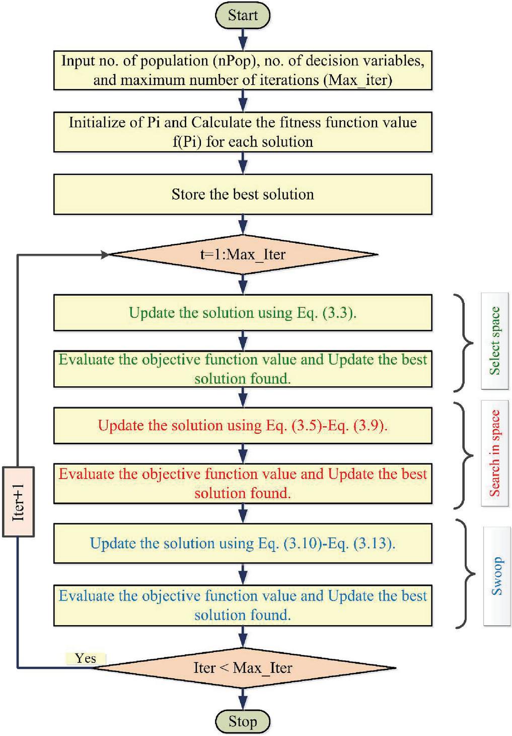
Figure 3 Flowchart of IBES.
The PSO algorithm is good at exploitation but not so good at exploration. Furthermore, exploitation implies that the algorithm does a very good local search. Exploration ability, on the other hand, boosts its ability to discover suitable starting positions, maybe around the global minimum. As a result, a well-designed algorithm strikes a balance between exploitation and exploration. PSO suffers from converging to a local minimum due to exploration capabilities when the starting location of the PSO algorithm is distant from the global minimum.
3.2 An Improved Bald Eagle Search Technique
Based on the bald eagle search algorithm [24], the improved bald eagle search (IBES) algorithm is inspired by bald eagle search behavior during the hunting phase [25] and the flowchart of IBES algorithm is given in Figure 3. The hunting technique is divided into three stages: selecting the space, searching the space, and finally swooping in on the prey.
Selecting the space: Based on the previous search information, the bald selects the space at random.
| (11) |
Instead of having a fixed value in the original BES method, the parameter alpha for managing position changes can be derived using the following equation.
| (12) |
This parameter influences the bald position of eagles and improves exploration and exploitation in the IBES approach. r is a number between 0 and 1. The new and current search spaces are denoted by p and p, respectively. p shows that these eagles have consumed all the information from the previous.
Search stage: To speed up their search for prey in this area, the eagles move in a spiral form. At this point, the eagle’s location is updated using Equation.
| (13) | |
| (14) | |
| (15) | |
| (16) | |
| (17) |
where is a parameter with a range of 5 to 10, and R is a parameter with a range of 0.5 to 2.
Swooping stage: At this stage, the eagles begin to swing from the optimal search position towards their prey, as expressed in Equation.
| (18) | |
| (19) | |
| (20) | |
| (21) |
where, and have value from 1 to 2.
4 Results
To carry out this work, MATLAB 2018a programming language has been used, which is installed in a computer window 8.1, intel i7 processor, 2.4GHz clock speed with 4GB Ram.
Table 7 LCI of 34 bus system and bus order based on CSIDI for IEEE34 Bus system
| C-1 | C-2 | C-3 | |||||||||
| Bus No. | LCI | Bus Order | CSIDI | Bus No. | LCI | Bus Order | CSIDI | Bus No. | LCI | Bus Order | CSIDI |
| 1 | Inf | 19 | 0.933 | 1 | Inf | 17 | 0.700 | 1 | Inf | 18 | 0.516 |
| 2 | 0.833 | 17 | 0.700 | 2 | 0.050 | 18 | 0.516 | 2 | 0.500 | 15 | 0.450 |
| 3 | Inf | 18 | 0.516 | 3 | Inf | 19 | 0.333 | 3 | 0.666 | 19 | 0.333 |
| 4 | 0.050 | 13 | 0.233 | 4 | 0.500 | 9 | 0.183 | 4 | Inf | 17 | 0.250 |
| 5 | 0.666 | 10 | 0.200 | 5 | 0.033 | 5 | 0.116 | 5 | Inf | 28 | 0.116 |
| 6 | 0.166 | 28 | 0.116 | 6 | 0.333 | 31 | 0.050 | 6 | 0.333 | 21 | 0.050 |
| 7 | 0.833 | 30 | 0.083 | 7 | 0.833 | 2 | 0 | 7 | 0.833 | 32 | 0.050 |
| 8 | 0.666 | 4 | 0.050 | 8 | 0.666 | 6 | 0.183 | 8 | 0.666 | 25 | 0.016 |
| 9 | 0.333 | 32 | 0.050 | 9 | 0.066 | 28 | 0.183 | 9 | 0.666 | 3 | 0.166 |
| 10 | 0.050 | 6 | 0.016 | 10 | 0.500 | 29 | 0.233 | 10 | 0.500 | 6 | 0.183 |
| 11 | Inf | 24 | 0.033 | 11 | Inf | 30 | 0.233 | 11 | Inf | 29 | 0.233 |
| 12 | 0.666 | 9 | 0.083 | 12 | 0.666 | 10 | 0.250 | 12 | 0.666 | 30 | 0.233 |
| 13 | 0.066 | 29 | 0.233 | 13 | 0.666 | 34 | 0.283 | 13 | 0.666 | 10 | 0.250 |
| 14 | 1 | 31 | 0.233 | 14 | 1 | 15 | 0.333 | 14 | 1 | 34 | 0.283 |
| 15 | 0.833 | 34 | 0.283 | 15 | 0.833 | 20 | 0.350 | 15 | 0.050 | 20 | 0.350 |
| 16 | Inf | 15 | 0.333 | 16 | Inf | 13 | 0.366 | 16 | Inf | 13 | 0.366 |
| 17 | 0.050 | 20 | 0.350 | 17 | 0.050 | 4 | 0.400 | 17 | 0.500 | 31 | 0.400 |
| 18 | 0.333 | 12 | 0.416 | 18 | 0.333 | 32 | 0.400 | 18 | 0.333 | 9 | 0.416 |
| 19 | 0.066 | 8 | 0.466 | 19 | 0.666 | 12 | 0.416 | 19 | 0.666 | 12 | 0.416 |
| 20 | 0.500 | 5 | 0.516 | 20 | 0.500 | 8 | 0.466 | 20 | 0.500 | 2 | 0.450 |
| 21 | 0.666 | 21 | 0.566 | 21 | 0.666 | 21 | 0.566 | 21 | 0.050 | 8 | 0.466 |
| 22 | Inf | 14 | 0.600 | 22 | Inf | 14 | 0.600 | 22 | Inf | 14 | 0.600 |
| 23 | 0.833 | 26 | 0.616 | 23 | 0.833 | 26 | 0.616 | 23 | 0.833 | 26 | 0.616 |
| 24 | 0.083 | 33 | 0.616 | 24 | 0.833 | 33 | 0.616 | 24 | 0.833 | 33 | 0.616 |
| 25 | 1 | 7 | 0.633 | 25 | 1 | 7 | 0.633 | 25 | 0.066 | 7 | 0.633 |
| 26 | 0.666 | 27 | 0.683 | 26 | 0.666 | 27 | 0.683 | 26 | 0.666 | 27 | 0.683 |
| 27 | 0.833 | 2 | 0.783 | 27 | 0.833 | 23 | 0.783 | 27 | 0.833 | 23 | 0.783 |
| 28 | 0.033 | 23 | 0.783 | 28 | 0.333 | 24 | 0.783 | 28 | 0.033 | 24 | 0.783 |
| 29 | 0.333 | 25 | 0.950 | 29 | 0.333 | 25 | 0.950 | 29 | 0.333 | 1 | Inf |
| 30 | 0.016 | 1 | Inf | 30 | 0.333 | 1 | Inf | 30 | 0.333 | 4 | Inf |
| 31 | 0.333 | 3 | Inf | 31 | 0.050 | 3 | Inf | 31 | 0.500 | 5 | Inf |
| 32 | 0.050 | 11 | Inf | 32 | 0.500 | 11 | Inf | 32 | 0.050 | 11 | Inf |
| 33 | 0.666 | 16 | Inf | 33 | 0.666 | 16 | Inf | 33 | 0.666 | 16 | Inf |
| 34 | 0.333 | 22 | Inf | 34 | 0.333 | 22 | Inf | 34 | 0.333 | 22 | Inf |
4.1 Results of CSIDI
The number of charging stations has been determined based on the data provided for the proposed region, as shown in Table 3. Furthermore, as mentioned in Section 2, the CSIDI value is determined for each bus in the distribution system. As a result, the LCI for land cost is depicted in Table 4 for three cases, and certain locations do not have land for FCS installation, which is represented by infinite. Furthermore, the value of CSIDI increases from top to bottom, as shown in Table 4 by the bus number. As a result of the low land cost and large EV population, the top buses have the highest priority for placing the FCS. Case-1 (C-1) utilizes the top eight buses to find a feasible position in the optimization problem, whereas Case-2 (C-2) likewise uses the top eight buses to find the optimal location of FCS. Furthermore, case-3 (C-3) looked for the best location of FCS among the top eight buses, as shown in Table 4. In a conclusion, the study for the optimal location of FCSs on the distribution system in the first stage has decreased the searching space for the optimization problem. In addition, the power loss is chosen as an objective function for optimal position. Furthermore, the land cost and EV population have been considered in the selection for the best placement of FCS on the distribution system.
As previously noted, the number of possible FCS locations has been decreased from 33 to 8. Following that, the three best locations on the distribution system from the obtained possible locations were selected by minimizing power loss with some distribution limits. As a result, the IEEE 34 bus distribution system proved the efficacy of the suggested FCS planning. The IEEE 34 distribution system proposed includes active power demands of 4636.5 kW and reactive power loads of 2873.5 kVAR. The backward forward flow algorithm is used in this study to calculate power flow. Furthermore, total active power loss (221.72 kW), lowest voltage (0.94171 at 27), and highest voltage (0.99414 at 2) are acquired values for the proposed distribution network without any FCS and SPDG installation.
4.2 Results of Optimal Location of FCS Using IBES Technique
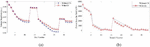
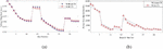
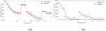
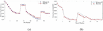
According to the previously acquired data, there were eight (19,17,18,13,10, 28,30,4) buses available for FCS installation. Furthermore, the findings for the optimal location of FCS have been achieved by reducing the power loss in C-1 utilizing the previously suggested PSO techniques. Figures 4(a) and 4(b) show the voltage at each bus and the power flow in each line. Furthermore, by reducing power loss, the optimal position of FCS from the possible buses was identified. As a result, Table 5 represents total power loss, minimum voltage, and optimal location on distribution network buses. The acquired bus voltage and power flow data for C-2 are shown in Figures 5(a) and 5(b). Eventually, the obtained results from the PSO algorithm for optimal location of FCSs by minimizing power loss are illustrated in Table 5 for C-3, while the optimal location of FCSs at buses 15, 17, and 18 have total active power losses (221.90 kW), minimum voltage (0.94378 at 27), and maximum voltage (0.99365 at 2). Furthermore, Figures 6(a) and 6(b) show the voltage and power flow findings for buses and lines, respectively.
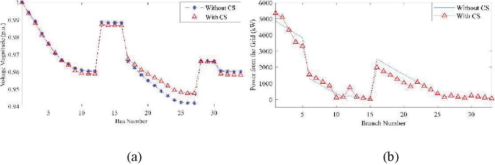
Figure 4 The bus voltage and power flow using PSO in C-1.
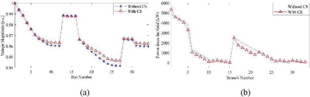
Figure 5 The bus voltage and power flow using PSO in C-2.
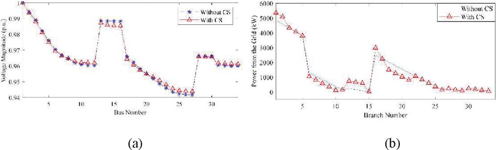
Figure 6 The bus voltage and power flow using PSO in C-3.
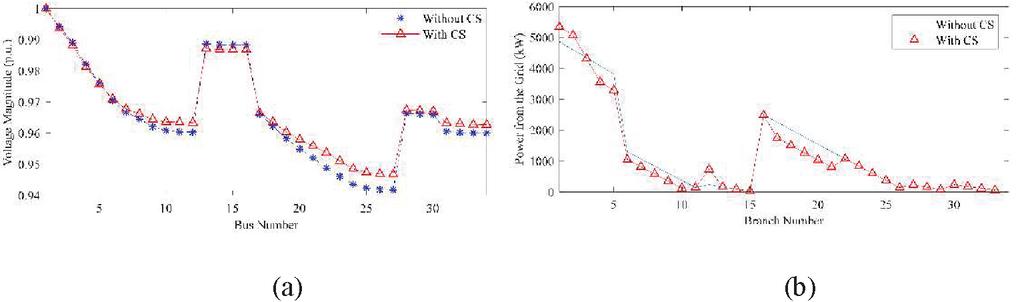
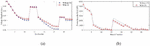
Figure 7 The bus voltage and power flow using IBES in C-1.
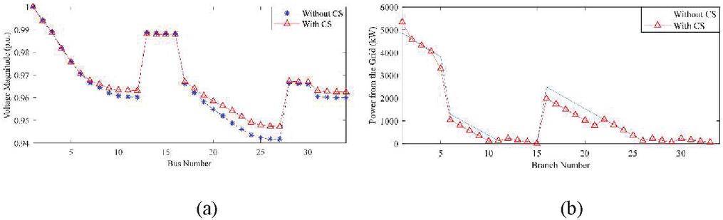
Figure 8 The bus voltage and power flow using IBES in C-2.
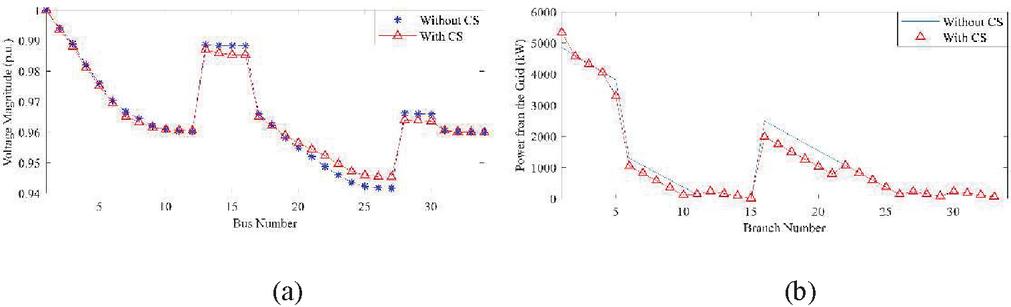
Figure 9 The bus voltage and power flow using IBES in C-3.
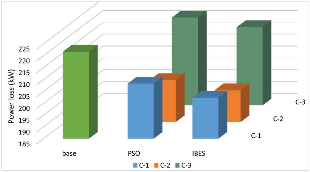
Figure 10 Power loss in different cases.
4.3 Results of Optimal Location for FCS Using IBES Technique
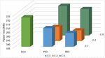
Furthermore, the IBES algorithm has recommended a suitable location for the FCS problem. The findings for the optimal location of FCS on the 4,13,17 bus for reducing power loss while maintaining voltage and power limitations were obtained in C-1. As a result, the minimum voltage at each bus and power flow in each line are shown in Figures 7(a) and 7(b). As already described. The authors obtained some improvements in the IBES technique results, including a 2.68% reduction in power loss. Furthermore, with a power loss of 198.43 kW, the optimal position of FCSs was found to be at 2, 5, 6 in C-2. Figures 8(a) and 8(b) suggest the voltage at each bus and the power flow in each line for optimal FCS position. Furthermore, the IBES approach reduced power loss by 1.89% when compared to PSO. Eventually, the optimal FCS position findings were achieved with a power loss of 217.85 kW. whereas the obtained voltage at each bus and power flow in each line are shown in Figures 9(a) and 9(b) for C-3. As a result, the IBES algorithm achieves a power loss decrease of 1.52%. Power loss for different cases is represented in Figure 10.
5 Conclusion and Recommendation
The purpose of this research was to integrate FCS into a distribution network with randomly distributed solar power generation (SPDG) utilizing an IBES optimization technique. The optimization problem was simulated using MATLAB 2018a. The objective was to optimally locate the FCSs so that they would not impact network quality. The objective functions were developed to decrease active power losses, investment costs and maximize the EV population. The SPDGs were randomly sized and sited using Microsoft Excel and then uploaded to MATLAB. When the results of the PSO and BES algorithms are examined, the significance of IBES is verified for the benchmark functions. In all three cases, the simulation results demonstrated the effectiveness of the IBES for obtaining the best locations for the installation of the FCSs across the distribution network. The performance of the IBES was validated by measuring its findings to those obtained while employing PSO for the placement of FCSs in the distribution network with randomly sized and located SPDGs. The simulation results show that the suggested IBES is an effective optimization approach for the placement of FCSs in current distribution networks with random SPDGs.
Table 8 Results comparison in three scenarios for the IEEE34 bus system
| PSO | IBES | ||||||
| — | Base Case | C-1 | C-2 | C-3 | C-1 | C-2 | C-3 |
| Power loss (kW) | 221.72 | 208.32 | 202.75 | 221.90 | 202.34 | 198.43 | 217.85 |
| Min. Voltage (p.u.) | 0.94171 at bus 27 | 0.94854 at bus 27 | 0.94651 at bus 27 | 0.94378 at bus 27 | 0.94678 at bus 27 | 0.94752 at bus 27 | 0.94542 at bus 27 |
| Max. Voltage (p.u.) | 0.99414 at bus 2 | 0.99372 at bus 2 | 0.99367 at bus 2 | 0.99365 at bus 2 | 0.99369 at bus 2 | 0.99372 at bus 2 | 0.99373 at bus 2 |
| FCSs location | – | 4,10,17 | 2,5,17 | 15,17,18 | 4,13,17 | 2,5,6 | 15,7,28 |
The future scope of this research will address the daylight variation of solar power generation, EV user driving patterns, distribution network uncertainties, and EV charging time for the best allocation of FCSs in the distribution network.
Acknowledgement
This publication was made possible by NPRP grant # [13S-0108-20008] from the Qatar National Research Fund (a member of Qatar Foundation). The statements made herein are solely the responsibility of the authors.
References
[1] N. Parker, H. L. Breetz, D. Salon, M. W. Conway, J. Williams, and M. Patterson, “Who saves money buying electric vehicles? Heterogeneity in total cost of ownership,” Transp. Res. Part D Transp. Environ., vol. 96, no. May, p. 102893, 2021, doi: 10.1016/j.trd.2021.102893.
[2] “When will fossil fuels run out?” https://group.met.com/fyouture/when-will-fossil-fuels-run-out/68 (accessed Dec. 26, 2021).
[3] N. Rietmann, B. Hügler, and T. Lieven, “Forecasting the trajectory of electric vehicle sales and the consequences for worldwide CO2 emissions,” J. Clean. Prod., vol. 261, p. 121038, 2020, doi: 10.1016/j.jclepro.2020.121038.
[4] S. Deb, K. Tammi, K. Kalita, and P. Mahanta, “Impact of electric vehicle charging station load on distribution network,” Energies, vol. 11, no. 1, pp. 1–25, 2018, doi: 10.3390/en11010178.
[5] H. Zhang, Z. Hu, Z. Xu, and Y. Song, “An integrated planning framework for different types of PEV charging facilities in urban area,” IEEE Trans. Smart Grid, vol. 7, no. 5, pp. 2273–2284, 2016, doi: 10.1109/TSG.2015.2436069.
[6] M. Z. Zeb et al., “Optimal placement of electric vehicle charging stations in the active distribution network,” IEEE Access, vol. 8, pp. 68124–68134, 2020, doi: 10.1109/ACCESS.2020.2984127.
[7] Dubey, Anamika and Surya Santoso. “Electric Vehicle Charging on Residential Distribution Systems: Impacts and Mitigations.” IEEE Access, vol. 3536, no. c, pp. 1–22, 2015, doi: 10.1109/ACCESS.2015.2476996.
[8] Betancur, Daniel, et al. “Methodology to Evaluate the Impact of Electric Vehicles on Electrical Networks Using Monte Carlo.” Energies, vol. 14, no. 5, p. 1300, 2021.
[9] L. Chen, C. Xu, H. Song, and K. Jermsittiparsert, “Optimal sizing and sitting of EVCS in the distribution system using metaheuristics: A case study,” Energy Reports, vol. 7, pp. 208–217, 2021, doi: 10.1016/j.egyr.2020.12.032.
[10] H. Simorgh, H. Doagou-Mojarrad, H. Razmi, and G. B. Gharehpetian, “Cost-based optimal siting and sizing of electric vehicle charging stations considering demand response programmes,” IET Gener. Transm. Distrib., vol. 12, no. 8, pp. 1712–1720, 2018, doi: 10.1049/iet-gtd.2017.1663.
[11] G. Battapothula, C. Yammani, and S. Maheswarapu, “Multi-objective simultaneous optimal planning of electrical vehicle fast charging stations and DGs in distribution system,” J. Mod. Power Syst. Clean Energy, vol. 7, no. 4, pp. 923–934, 2019, doi: 10.1007/s40565-018-0493-2.
[12] M. H. Amini, M. P. Moghaddam, and O. Karabasoglu, “Simultaneous allocation of electric vehicles’ parking lots and distributed renewable resources in smart power distribution networks,” Sustain. Cities Soc., vol. 28, pp. 332–342, 2017, doi: 10.1016/j.scs.2016.10.006.
[13] Shukla, Akanksha, et al. “Multi-Objective Synergistic Planning of EV Fast-Charging Stations in the Distribution System Coupled with the Transportation Network.” IET Generation, Transmission and Distribution, vol. 13, no. 15, pp. 3421–3432, 2019, doi: 10.1049/iet-gtd.2019.0486.
[14] S. Deb, S. Member, K. Tammi, X. Gao, K. Kalita, and P. Mahanta, “A hybrid multi-objective chicken swarm optimization and teaching learning based algorithm for charging station placement problem,” IEEE Access, vol. 8, pp. 92573–92590, 2020, doi: 10.1109/ACCESS.2020.2994298.
[15] F. Ahmad, A. Iqbal, I. Ashraf, M. Marzband, and I. khan, “Optimal location of electric vehicle charging station and its impact on distribution network: A review,” Energy Reports, vol. 8, pp. 2314–2333, Nov. 2022, doi: 10.1016/J.EGYR.2022.01.180.
[16] H. Zhang, S. J. Moura, Z. Hu, and Y. Song, “PEV fast-charging station siting and sizing on coupled transportation and power networks,” IEEE Trans. Smart Grid, vol. 9, no. 4, pp. 2595–2605, 2018, doi: 10.1109/TSG.2016.2614939.
[17] A. Eid, “Allocation of distributed generations in radial distribution systems using adaptive PSO and modified GSA multi-objective optimizations,” Alexandria Eng. J., vol. 59, no. September, pp. 4771–4786, 2020, doi: 10.1016/j.aej.2020.08.042.
[18] Y. Wang, J. Shi, R. Wang, Z. Liu, and L. Wang, “Siting and sizing of fast charging stations in highway network with budget constraint,” Appl. Energy, vol. 228, no. April, pp. 1255–1271, 2018, doi: 10.1016/j.apenergy.2018.07.025.
[19] L. Liu, F. Xie, Z. Huang, and M. Wang, “Multi-objective coordinated optimal allocation of DG and evcss based on the V2G mode,” Processes, vol. 9, no. 1, pp. 1–18, 2021, doi: 10.3390/pr9010018.
[20] S. R. Gampa, K. Jasthi, P. Goli, D. Das, and R. C. Bansal, “Grasshopper optimization algorithm based two stage fuzzy multiobjective approach for optimum sizing and placement of distributed generations, shunt capacitors and electric vehicle charging stations,” J. Energy Storage, vol. 27, no. November 2019, p. 101117, 2020, doi: 10.1016/j.est.2019.101117.
[21] P. Phonrattanasak and N. Leeprechanon, “Optimal location of fast charging station on residential distribution grid,” Int. J. Innov. Manag. Technol., vol. 3, no. 6, p. 675, 2012, doi: 10.7763/IJIMT.2012.V3.318.
[22] “When fossil fuels run out, what then? – MAHB.” https://mahb.stanford.edu/library-item/fossil-fuels-run/ (accessed Dec. 26, 2021).
[23] J. Kennedy and R. Eberhart, “Particle swarm optimization,” ICNN’95-international Conf. neural networks, vol. 4, pp. 1942–1948, 1995.
[24] H. A. Alsattar, A. A. Zaidan, and B. B. Zaidan, “Novel meta-heuristic bald eagle search optimisation algorithm,” Artif. Intell. Rev., vol. 53, no. 3, pp. 2237–2264, 2020, doi: 10.1007/s10462-019-09732-5.
[25] A. Ramadan, S. Kamel, M. H. Hassan, T. Khurshaid, and C. Rahmann, “An improved bald eagle search algorithm for parameter estimation of different photovoltaic models,” Processes, vol. 9, no. 7, 2021, doi: 10.3390/pr9071127.
Biographies

Fareed Ahmad received his master’s degree in Electrical Engineering (M.Tech) in the specialization of instrumentation and control in 2016 from Aligarh Muslim University, Aligarh, India, and Bachelor of Engineering (B.Tech) degree in Electrical Engineering from Gautama Buddha Technical University (GBTU), India in 2013. Currently, he is a Research Scholar (Ph.D. candidate) in the Electrical Engineering Department of Zakir Hussain College of Engineering & Technology at Aligarh Muslim University, India.

Atif Iqbal, Fellow IET (UK), Fellow IE (India) and Senior Member IEEE, Vice-Chair, IEEE Qatar section, DSc (Poland), Ph.D. (UK) – Associate Editor, IEEE Trans. On Industrial Electronics, IEEE ACCESS, Editor-in-Chief, I ‘manager Journal of Electrical Engineering, Former Associate Editor IEEE Trans. On Industry Application, Former Guest Associate Editor IEEE Trans. On Power Electronics. Full Professor at the Dept. of Electrical Engineering, Qatar University and Former Full Professor at the Dept. of Electrical Engineering, Aligarh Muslim University (AMU), Aligarh, India. Recipient of Outstanding Faculty Merit Award academic year 2014–2015 and Research excellence awards 2015 and 2019 at Qatar University, Doha, Qatar. He received his B.Sc. (Gold Medal) and M.Sc. Engineering (Power System & Drives) degrees in 1991 and 1996, respectively, from the Aligarh Muslim University (AMU), Aligarh, India, and Ph.D. in 2006 from Liverpool John Moores University, Liverpool, UK. He obtained DSc (Habilitation) from Gdansk University of Technology in Control, Informatics and Electrical Engineering in 2019. He has been employed as a Lecturer in the Department of Electrical Engineering, AMU, Aligarh since 1991 where he served as Full Professor until Aug. 2016. He is recipient of Maulana Tufail Ahmad Gold Medal for standing first at B.Sc. Engg. (Electrical) Exams in 1991 from AMU. He has received several best research papers awards e.g. at IEEE ICIT-2013, IET-SEISCON-2013, SIGMA 2018, IEEE CENCON 2019, IEEE ICIOT 2020, ICSTEESD-20 and Springer ICRP 2020. He has published widely in International Journals and Conferences his research findings related to Power Electronics, Variable Speed Drives and Renewable Energy Sources. Dr. Iqbal has authored/co-authored more than 450 research papers and four books and several chapters in edited books. He has supervised several large R&D projects worth more than multimillion USD. He has supervised and co-supervised several Ph.D. students. His principal area of research interest is Smart Grid, Complex Energy Transition, Active Distribution Network, Electric Vehicles drivetrain, Sustainable Development and Energy Security, Distributed Energy Generation and multiphase motor drive system.

Imtiaz Ashraf was born in India in 1965. He received his B. Sc. Engg. and M.Sc. Engg. (Electrical Engineering) degrees in 1988 and 1993 respectively from Zakir Husain College of Engineering and Technology, Aligarh Muslim University (AMU), Aligarh, India. He received his Ph.D. degree from the Indian Institute of Technology, Delhi, India in 2005. Presently he is a Professor and Chairman in Electrical Engineering Department, AMU, Aligarh, India. His area of interest is Energy Systems, Electrical Power Systems, Energetics, Economics and Environmental assessment of renewable energy sources.
Mousa Marzband (Senior Member, IEEE) received a Ph.D. degree in power system engineering from the Universitat Politècnica de Catalunya (UPC), in 2014. Following that, he started a Postdoctoral Fellowship at the University of Manchester (UoM), and the University College Cork’s Environmental Research Institute and Marine and Renewable Energy (MaREI) Ireland. Since August 2017, he has been appointed as an Assistant Professor (Lecturer) with the Department of Mathematical, Physics and Electrical Engineering, Northumbria University, the U.K., where he is currently a Senior Lecturer. In addition, he received the Distinguished Adjunct Professor Award from the Engineering School, King Abdulaziz University, in 2019.

Irfan Khan (Member, IEEE) received a Ph.D. degree in electrical and computer engineering from Carnegie Mellon University, USA. He is currently an Assistant Professor of Practice with the Electrical and Computer Engineering Department, Texas A&M University (TAMU), TX, USA. He has published more than 20 refereed journal and conference papers in smart energy systems related areas. His current research interests include control and optimization of smart energy networks, optimization of energy storage systems, DC micro grids, smart grids, and renewable energy resources. He is a member of PES. He is the Vice Chair for the IEEE PES Joint Chapter of Region 5 Galveston Bay Section (GBS), where his responsibilities are to organize presentations, invite renowned experts from power and energy background for presentations to GBS members. He is the Registration Chair at the IEEE sponsored International Symposium on Measurement and Control in Robotics that was organized at the University of Houston Clear Lake on September 19–21, 2019. He is an active Reviewer of many esteemed journals and conferences, including the IEEE Transactions on Power Systems, the IEEE Transactions on Smart Grids, IEEE Access, the IEEE Transactions on Industry Application Systems, IET Smart Grids, Electrical Power Components and Systems, and Energies.
Distributed Generation & Alternative Energy Journal, Vol. 37_4, 1277–1304.
doi: 10.13052/dgaej2156-3306.37416
© 2022 River Publishers