Data Mining and Machine Learning Technique in Contingency Analysis of Power System with UPFC

Ravi V. Angadi^1,*, Suresh Babu Daram², P. S Venkataramu¹ and V Joshi Manohar¹

¹Department of Electrical and Electronics Engineering, Presidency University, Bengaluru, Karnataka, India
²Department of Electrical and Electronics Engineering, Sree Vidyanikethan Engineering College, Tirupati, AP, India
E-mail: raviangadi404@gmail.com; sureshbabudaram@gmail.com; venkataramups1@gmail.com; joshimanohar@presidencyuniversity.in
*Corresponding Author

Received 30 August 2021; Accepted 09 December 2021; Publication 24 May 2022

Abstract

This paper explains how to predict the severity of the system by connecting with and without a unified power flow controller under different load and n-1 conditions by calculating the LVSI and by the application of data mining and machine learning techniques. A large amount of data will occur during the process of contingency analysis and it is necessary that how to get this to the system value to assess the severity of the system. With the help of data mining and machine learning techniques, analysis of data generated from the simulations for different load conditions are carried out and is used to estimate the severity of the line. In this, the IEEE 30 Bus System is used by calculating the line voltage stability index and the simulation work is carried out by using MATLAB and WEKA software.

Keywords: Contingency analysis, LVSI, data mining, machine learning, severity prediction.

1 Introduction

It is difficult to manage the power system in the world due to its complexity to manage and control large power systems. The continuous rise in demand of power consumption, it is inevitable to interconnect and extend the transmission networks. This leads to the difficult challenge of proper functioning of the power system to meet the consumer’s requirements to supply power at the required voltage and frequency. To achieve this, power system should operate with high security by using the real time applications, in order to take proper corrective steps to ensure the system’s smooth running.

It is necessary to overcome from the severe problems like unexpected line loss or generator failure, unexpected increase or decrease in power demand in normally working power system [1]. To do this, FACTS devices are used in the system to maintain the stability of the power system by maintaining the voltage profile [2]. In this case, the line is incorporated with and without FACTS device i.e., connecting UPFC with the help of load flow study, to provide the necessary compensation to maintain the stability the system is briefed in [3–5]. During the contingency analysis, a large amount of data will be produced and this data will be used effectively to bring it to the system value. By the application of data analytics, contingency study is done for different load and contingency conditions. The severity of the line is predicted by processing and pre-processing the data, later it fed to the machine learning tool [6–8].

2 Contingency Analysis and Ranking

The contingency analysis is one of the main components for energy management. The system stability soon after breakdown scan is esteemed efficiently by the research of the contingency analysis. CA is used to find out the impacts of future breakdowns and this helps to show the effects of potential failures to the operators [9, 10]. The failure occurs due to the sudden open in the transmission line, tripping the generator, sudden change in generation and change the load value suddenly. Due to the increased demand in a stable electricity supply and the growth of transmission system, the power system facing a number of limitations. To overcome from this the contingency analysis is required to analyse the problems [11].

“The analysis of contingency is obtained by using load flow analysis. The load flow solution will provide the active, reactive power flows & bus voltage magnitudes by NR method. The line-out result and the contingency rating method were found in the power system” [12, 13]. The contingency is determined and listed, based on the resulting index, commencing with the maximum value of the performance index. The stability index of every line calculated in this article is a line voltage index for contingency analysis. In accordance with the final reactive power and reactance power of the various lines, the voltage stability index for a particular line.

3 Contingency Analysis Using Data Processing and Data Mining

Data handling is the big task at present days as use of data extraction techniques has quickly expanded, by converting the raw data into valuable knowledge. Data mining is a technique of detection by big data sets of patterns and other important information. Despite its continued development in data-handling, however, leaders continue to confront problems with scalability and automation [14, 15]. Data mining approaches that support this analysis may be separated into two key goals, either by describing a target dataset or by using algorithms to predict results [16].

The data mining method helps the power engineers to find relevant data, pattern observations and links. The Data mining comprises generally of four basic steps: objectives setting, data collection and processing; application of data mining techniques; and outcomes evaluation [17, 18]. In the study of contingency analysis of power system, a lots of simulations works will be carried out in order to know the load flows of the system for different loading conditions with and without FACTS Devices. In this process a lot of data handling will be required, the data mining techniques will be suits more too contingency study of power system described in [6, 7, 19].

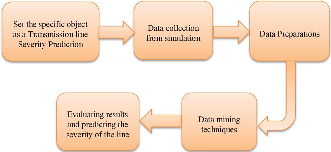
Figure 1 Data mining process applied to contingency study of power system.

The Figure 1 shows the schematic process flow of data mining techniques that is applied to contingency analysis of power system. The first stage of data mining process is set the specific object, this might be the trickiest component of the data mining process, and too little effort should be needed. Before evaluating data, data must first be collected. This method may differ for the purpose of utilizing the data from one system to another. In this initial stage three sorts of data are collected: a. structured data b. Un-structured data c. Semi-structured data.

The second stage of the data mining process is to collect the data set from the simulation process as per the required format and in the third stage of process it easily selects which datasets can assist the power engineers in answering the relevant questions. A further step can be taken to limit the number of dimensions, as too many characteristics slow down any future calculations, depending on the dataset. While high frequency patterns have wider uses, the data variations might be occasionally more intriguing to indicate possible severity predictions.

In the fourth stage of data mining process a data set classifying or clustering may be applied, in this case it is proposed to use classification algorithms based on the given data. When labelling of the input data (i.e. supervised learning), a classification model may be used for the categorization of data or a regression can be employed, in order to predict the probability of a specific task.

In the last stage of the data mining process the findings must be reviewed and understood when the data is aggregated. They should be valid, new, practical and comprehensible when completing findings. When these requirements are fulfilled, proposed system may utilize this information to create new strategies to achieve the severity prediction of the transmission line in an effective manner.

4 Waikato Environment for Knowledge Analysis (WEKA)

A prominent Java-based machine learning software package created at the University of Waikato in New Zealand, Weka. Data analysis and predictive modelling are made easier using the Weka workbench, which includes a set of visualization tools and algorithms for data analysis and predictive modelling, as well as graphical user interfaces that make it simple for users to access this capability. To solve real-world data mining challenges, Weka is a set of machine learning algorithms that may be used. Written in Java, it can operate on practically any operating system. There are two ways to use the algorithms: either directly on a dataset or indirectly using Java code. There was also a Makefile-based framework for launching machine learning experiments, and a TCL/TK front-end to (mainly third-party) modelling algorithms implemented in other programming languages. However, the more current entirely Java-based version (Weka 3), for which development began in 1997, is now utilized in a wide range of application fields, particularly for educational and research reasons. Here are some of the benefits of utilizing Weka; a. Because it is entirely implemented in the Java programming language and thus operates on nearly any current computing platform, it has the advantage of portability. b. Under the terms of the GNU General Public License, this service is provided for free. c. A broad array of approaches for data preparation and modelling is available online. d. graphical user interfaces, which make it simple to utilize. Weka offers a wide range of conventional data mining operations, including data preparation, clustering, classification, and regression, visualization, and feature selection [20–22]. Everything Weka does is premised on the notion that data is provided as a single flat file or relation, with each data point being characterized by a set amount of characteristics, and that the data is available in the format of normally numeric or nominal attributes, but some other attribute types are also supported [23].

5 Proposed Algorithm

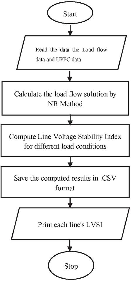
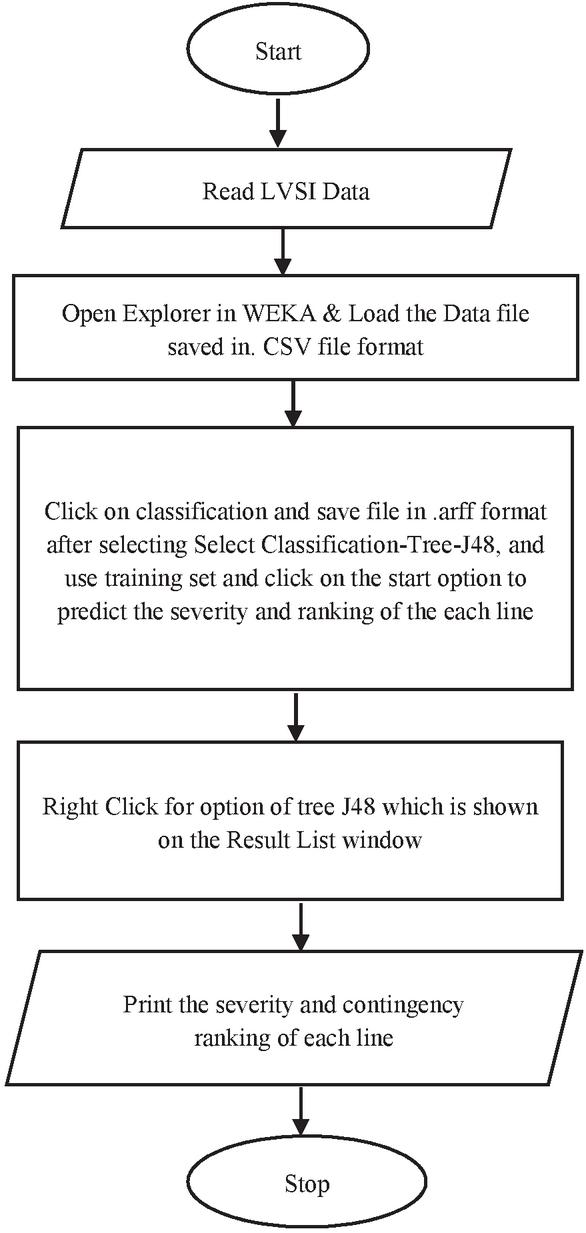
The application of UPFC mathematical modelling is explained by the suggested method [2–4]. The load flow solution Newton Raphson which includes UPFC into the system and equation based computerization of LVSI [6, 7]. The collected organized data is shown by the projected flow chart in Figure 2. The Figure 3 provides all the information examined, classified and forecast for the severity of the STLO using classification algorithm.

The supervised learning is one of the approaches in machine learning which predicts the link between the input and the target qualities. The supervised learning is used to assess the severity of the transmission line under various load conditions. The controlled approaches are grouped mostly into models like classification models and regression models.

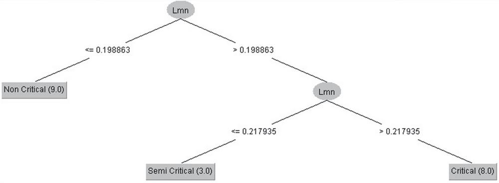
In order to define models of both classification and regression, a classification algorithm model may be used in operational data mining discussed in [24]. A comparative study of various classification approaches were discussed in [25–27]. In the proposed work j48 classification algorithm is considered for predicting the severity of the line. The Figure 7, shows the decision classification tree which includes root node, all leaf node and inner nodes describing requirements for examination. The end user can assess the numerous supports for data mining by this decision tree.

Figure 2 Flow chart to compute LVSI for given system .

Figure 3 Proposed Flow chart to predict the severity of transmission line using classification algorithm.

6 Case Study and Results

“The efficiency of the proposed method is examined by using the IEEE-30 bus system for simulation purposes. The convergence limit is 0.00001 for the active and reactive power. The system base MVA is 100 MVA. There are 1-slack buses, 5-generator buses, 24 cargo buses and 41 transmission lines for the IEEE-30 bus system” [7].

The effect of UPFC on voltage stability margin for a specific line contingency is as follows. The CN ranking was observed for different load conditions like 100% and 150%, with and without UPFC is analysed by NR method [28].

The load buses are incorporated with the UPFC and are connecting in line between bus-12. The effective values of the parameters r and $γ$ for the reduction of power loss in the system and to enhance the voltage profile are 0.1 & 1.85 respectively. The impedance of the series transformer connected in the line is considered as 0.1 pu. A total 32 contingencies are identified for a single transmission line outage contingency condition and under each contingency a particular transmission lines are made outage as per the Table 1.

Table 1 List of Contingency and Number of transmission line considered for contingency

			Transmission Line				Transmission Line
Sl. No	C No	L No.	From Bus	To Bus	Sl. No	C No	L No.	From Bus	To Bus
1	1	2	1	3	17	17	24	19	20
2	2	3	2	4	18	18	25	10	20
3	3	5	2	5	19	19	26	10	17
4	4	6	2	6	20	20	27	10	21
5	5	7	4	6	21	21	28	10	22
6	6	8	5	7	22	22	29	21	22
7	7	9	6	7	23	23	30	15	23
8	8	10	6	8	24	24	31	22	24
9	9	14	9	10	25	25	32	23	24
10	10	17	12	14	26	26	33	24	25
11	11	18	12	15	27	27	35	25	27
12	12	19	12	16	28	28	36	28	27
13	13	20	14	15	29	29	38	27	30
14	14	21	16	17	30	30	39	29	30
15	15	22	15	18	31	31	40	8	28
16	16	23	18	19	32	32	41	6	28
Note: C No: Contingency Number. L No: Line Number.

The ranking for the lines was based on this particular line on the line stability index value. The rankings are classified as mentioned in Table 2. The top 10 contingency ranks are tabulated in the Table 3 for different load condition with and without UPFC. Table 3 shows the increase in the condition number with the increase in system load. UPFC reduces the value of condition number. By connecting UPFC to the line no. 9 condition number is reduced under the base load condition. The same analysis was carried for different loading and observed it for top 10 contingency ranking is listed in the Table 3. The only contingency condition of the single transmission line is believed to follow the categorization approach in many circumstances. In this article to do two cases are considered during study. Case-1: System with load variation under single transmission line outage condition without and with UPFC. Case-2: System with 150% load variation under single transmission line outage condition without and with UPFC. The single line outages are considered into account separately to prepare the data for different loading conditions, in all two scenarios. The data produced is firstly pre-processed and categorized with j48 classification algorithms by ranging as critical, semi-critical and non-critical.

Table 2 Contingency ranking classification

Sl. No	Condition	Ranks
1	Critical	1 to 10
2	Semi	11 to 20
3	Non-critical	21 to 41

Table 3 Contingency Top 10 Ranking for different load condition

	100% Load Condition	120% Load Condition	150% Load Condition
	Line No/ CN/Lmn	Line No/ CN/Lmn	Line No/ CN/Lmn
Rank	Without	Without	Without	Without	Without	Without
No	UPFC	UPFC	UPFC	UPFC	UPFC	UPFC
1	9/14/0.3236	9/14/0.2832	9/14/0.5460	9/14/0.5425	3/5/0.71547	3/5/0.60071
2	1/2/0.32233	1/2/0.31565	1/2/0.43793	1/2/0.43133	9/14/0.6842	9/14/0.6590
3	3/5/0.30736	3/5/0.30591	3/5/0.41922	3/5/0.42271	5/7/0.52085	5/70.50391
4	4/6/0.25941	4/6/0.25917	4/6/0.40009	4/6/0.39888	32/41/0.462	32/41/0.448
5	2/3/0.25017	2/3/0.21406	2/3/0.38789	2/3/0.39833	31/40/0.451	0.44687
6	6/8/0.25017	6/8/0.21245	32/41/0.376	32/41/0.370	1/2/0.45033	1/2/0.45232
7	32/41/0.247	32/42/0.244	19/26/0.370	19/26/0.369	8/10/0.4157	8/10/0.3759
8	21/28/0.228	21/28/0.225	24/31/0.364	24/31/0.370	19/26/0.407	19/26/0.388
9	19/26/0.224	19/26/0.236	18/25/0.361	18/25/0.361	4/6/0.40514	4/6/0.38371
10	18/25/0.21793	18/25/0.23023	17/24/0.3564	17/24/0.35572	18/25/0.39	18/25/0.3

Table 4 Trained Data set for Base Load Condition with and without UPFC

Without UPFC					With UPFC
SL. No	C No	L No	Lmn	Condition	SL. No	C No	L No	Lmn	Condition
1	1	2	0.322331	Critical	21	1	2	0.31565	Critical
2	2	3	0.255147	Critical	22	2	3	0.21406	Semi Critical
3	3	4	0.321012	Critical	23	3	5	0.30591	Critical
4	4	5	0.307365	Critical	24	4	6	0.25917	Critical
5	5	6	0.2594	Critical	25	5	7	0.2244	Semi Critical
6	6	7	0.21755	Semi Critical	26	6	8	0.21245	Semi Critical
7	7	8	0.250169	Critical	27	7	9	0.18991	Non Critical
8	8	9	0.194066	Non Critical	28	8	10	0.18191	Non Critical
9	9	10	0.192362	Non Critical	29	9	14	0.28328	Critical
10	10	14	0.323621	Critical	30	10	17	0.20501	Semi Critical
11	11	17	0.192517	Non Critical	31	11	18	0.17929	Non Critical
12	12	18	0.166946	Non Critical	32	12	19	0.18475	Non Critical
13	13	19	0.172905	Non Critical	33	13	20	0.19255	Non Critical
14	14	20	0.196109	Non Critical	34	14	21	0.18231	Non Critical
15	15	21	0.186144	Non Critical	35	15	22	0.19561	Non Critical
16	16	22	0.183411	Non Critical	36	16	23	0.18741	Non Critical
17	17	23	0.191109	Non Critical	37	17	24	0.22594	Critical
18	18	24	0.21366	Semi Critical	38	18	25	0.23023	Critical
19	19	25	0.217935	Semi Critical	39	19	26	0.23629	Critical
20	20	26	0.224287	Critical	40	20	27	0.21847	Semi Critical

6.1 Case-1: Variation of 100% of Load in the System Under Single Transmission Line Outage Without and with UPFC

The severity was predicted based on LVSI which was computed for different load condition without and with incorporating UPFC, the data generated during this phenomenon was in high volume and was precessed with the help of data analytic and machine learning tools. In this analysis 60% of the data is used for training to predict the severity of the line and 30% of the data is used to test based on the training data set. Table 4 shows the training data set for the different load condition.

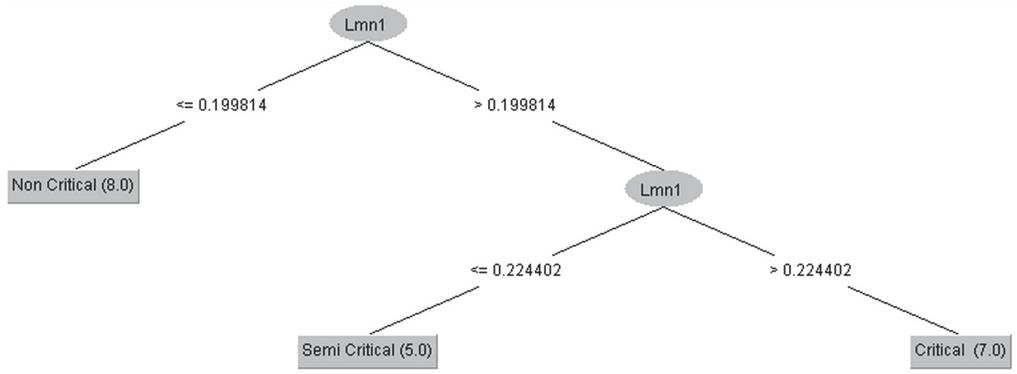
Figure 4 Decision tree for base loading condition without UPFC (Case-I).

Figure 5 Decision tree for base loading condition with UPFC (Case-I).

Table 5 Tested Data set For Base Load Condition with and without UPFC

Without UPFC					With UPFC
Sl. No	C. No	L No	Lmn	Condition	Sl. No	C. No	L No	Lmn	Condition
1	33	41	0.247597	Critical	1	32	41	0.244618	‘Critical’
2	22	28	0.228563	Critical	2	24	31	0.226844	‘Critical’
3	25	31	0.214959	‘Semi Critical’	3	21	28	0.225774	‘Critical’
4	21	27	0.206125	‘Semi Critical’	4	26	33	0.217019	‘Semi Critical’
5	27	33	0.204906	‘Semi Critical’	5	31	40	0.211999	‘Semi Critical’
6	32	40	0.198863	‘Non Critical’	6	30	39	0.209654	‘Semi Critical’
7	31	39	0.197123	‘Non Critical’	7	28	36	0.209494	‘Semi Critical’
8	29	37	0.196952	‘Non Critical’	8	29	38	0.209412	‘Semi Critical’
9	30	38	0.196862	‘Non Critical’	9	27	35	0.203364	‘Semi Critical’
10	23	29	0.195312	‘Non Critical’	10	23	30	0.199814	‘Non Critical’
11	26	32	0.193285	‘Non Critical’	11	22	29	0.191681	‘Non Critical’
12	28	35	0.191246	‘Non Critical’	12	25	32	0.189778	‘Non Critical’
13	24	30	0.187377	‘Non Critical’	13	–	–	–	–

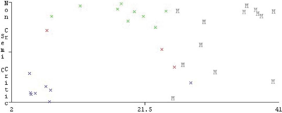
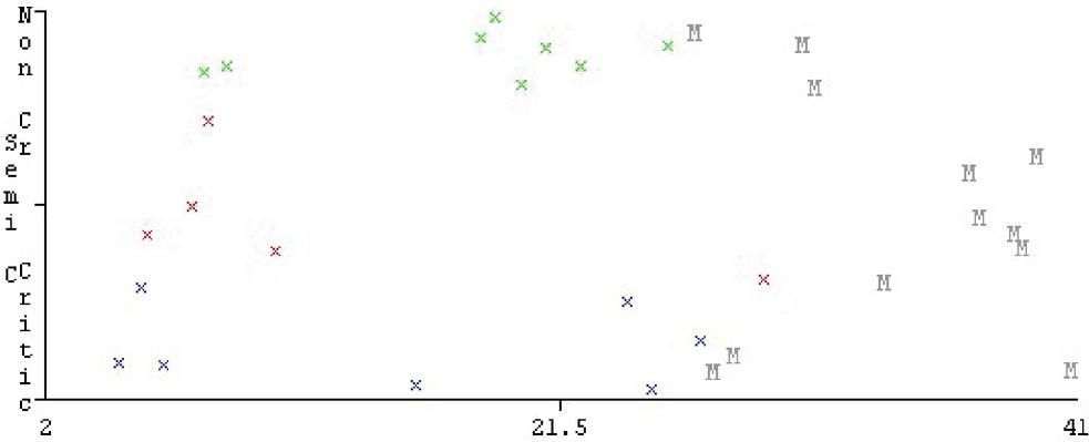
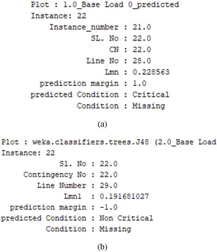
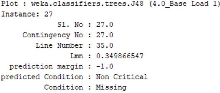
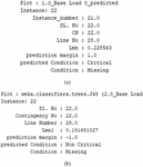
Figure 4 shows the decision tree chart for the basic loading condition without UPFC and Figure 5 for loading the basic load system with UPFC is illustrated. By considering the categorization, in Table 5, the critical, semi-critical and non-critical ranges are tabulated and severity forecast for the stabilization line voltage index are provided. The Figure 6 shows visualization classifier error for base load condition without UPFC under single line outage. Similarly, the visualization classifier error for base load condition with UPFC under single line outage is shown in the Figure 7. The data scattered visualization is obtained for different condition and analysed by using the visualization classifier errors. Based on the training data set, the sample missing data set condition and rank are predicted for the base load condition without UPFC under single line outage is shown in Figure 8(a). Similarly, the sample missing data set condition and rank are predicted for the base load condition with UPFC under single line outage is shown in the Figure 8(b).

Figure 6 Visualization of Condition versus line number for base load condition without UPFC.

Figure 7 Visualization of Condition versus line number for base load condition with UPFC.

Figure 8 (a) & (b) Sample missing data instant info for base load condition without and with UPFC.

6.2 Case-II: Variation of 150% of Load in the System Under Single Transmission Line Outage Without and with UPFC

The severity was predicted based on LVSI which was computed for different load condition without and with incorporating UPFC, the data generated during this phenomenon was in high volume and was processed with the help of data analytic and machine learning tools. In this analysis 60% of the data is used for training to predict the severity of the line and 30% of the data is used to test based on the training data set. Table 7 shows the training data set for the different load condition.

Table 6 Trained Data set for 150% Load Condition with and without UPFC

Without UPFC					With UPFC
SL. No	CN	L No	Lmn	Condition	SL. No	CN	L No	Lmn	Condition
1	1	2	0.4503	Critical	21	1	2	0.4503	Critical
2	2	3	0.3905	Semi Critical	22	2	3	0.3905	Semi Critical
3	3	5	0.7154	Critical	23	3	5	0.7154	Critical
4	4	6	0.4051	Critical	24	4	6	0.4051	Critical
5	5	7	0.5208	Critical	25	5	7	0.5208	Critical
6	6	8	0.3855	Semi Critical	26	6	8	0.3855	Semi Critical
7	7	9	0.3787	Semi Critical	27	7	9	0.3787	Semi Critical
8	8	10	0.4157	Critical	28	8	10	0.4157	Critical
9	9	14	0.6842	Critical	29	9	14	0.6842	Critical
10	10	17	0.348	Non Critical	30	10	17	0.3485	Non Critical
11	11	18	0.3198	Non Critical	31	11	18	0.3198	Non Critical
12	12	19	0.3201	Non Critical	32	12	19	0.3201	Non Critical
13	13	20	0.3550	Non Critical	33	13	20	0.3550	Non Critical
14	14	21	0.3427	Non Critical	34	14	21	0.342779833	Non Critical
15	15	22	0.3389	Non Critical	35	15	22	0.338926119	Non Critical
16	16	23	0.3465	Non Critical	36	16	23	0.34654	Non Critical
17	17	24	0.3775	Semi Critical	37	17	24	0.37758	Semi Critical
18	18	25	0.3951	Critical	38	18	25	0.39516	Critical
19	19	26	0.4078	Critical	39	19	26	0.40783	Critical
20	20	27	0.3800	Semi Critical	40	20	27	0.38002	Semi Critical

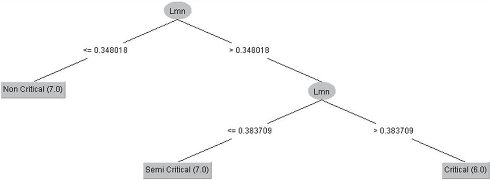
Figure 9 Decision tree for 150% load condition without UPFC (Case-II).

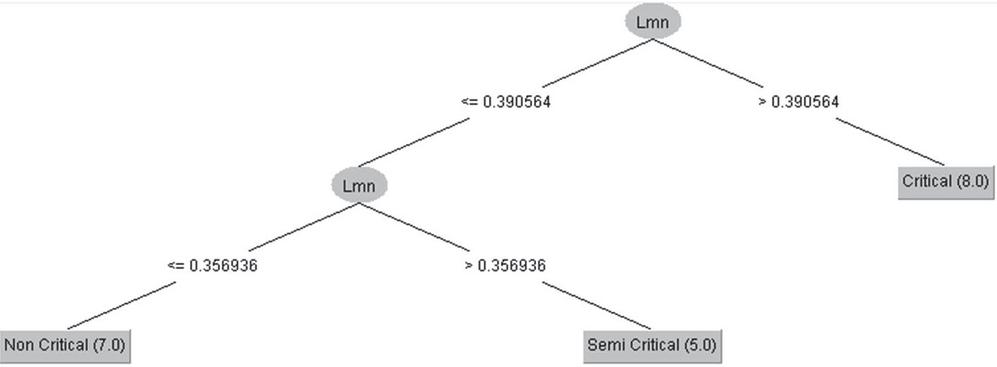
Figure 10 Decision tree for 150% load condition with UPFC (Case-II).

Table 7 Tested Data set For Base Load Condition with and without UPFC

Without UPFC					With UPFC
Sl. No	C. No	L No	Lmn	Condition	Sl. No	C. No	L No	Lmn	Condition
1	33	41	0.4487	Critical	1	32	41	0.4627	Critical
2	32	40	0.4468	Critical	2	31	40	0.4515	Critical
3	22	28	0.3910	Critical	3	24	31	0.3946	Critical
4	25	31	0.3870	Critical	4	21	28	0.3890	‘Semi Critical’
5	27	33	0.3613	‘Semi Critical’	5	26	33	0.3688	‘Semi Critical’
6	21	27	0.3605	‘Semi Critical’	6	28	37	0.3675	‘Semi Critical’
7	31	39	0.3486	‘Semi Critical’	7	29	38	0.3671	‘Semi Critical’
8	29	37	0.3480	‘Non Critical’	8	30	39	0.3569	‘Non Critical’
9	30	38	0.3475	‘Non Critical’	9	22	29	0.3548	‘Non Critical’
10	23	29	0.3466	‘Non Critical’	10	27	35	0.3498	‘Non Critical’
11	28	35	0.3409	‘Non Critical’	11	25	32	0.3486	‘Non Critical’
12	26	32	0.3402	‘Non Critical’	12	23	30	0.3449	‘Non Critical’
13	24	30	0.3366	‘Non Critical’	13	–	–	–	–

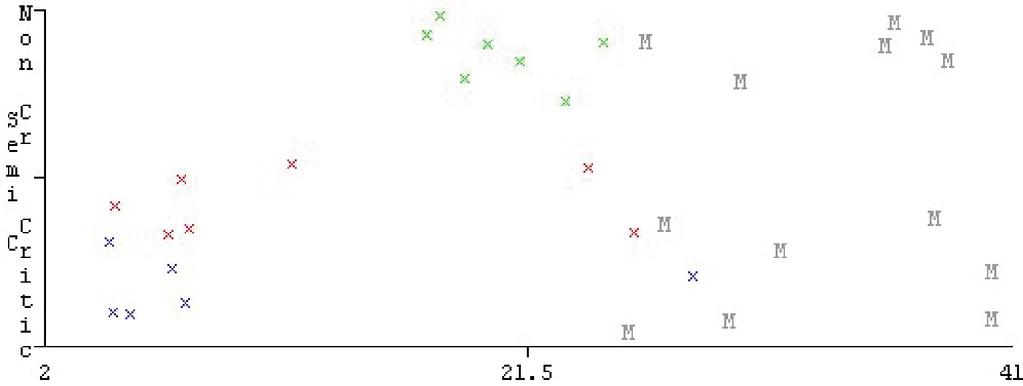
Figure 11 Visualization of Condition versus line number for 150% load condition without UPFC.

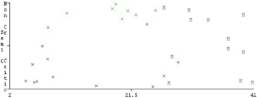
Figure 12 Visualization of Condition versus line number for 150% load condition with UPFC.

Figure 13 Sample missing data instant info for base load condition without and with UPFC.

Figure 9 show the decision tree chart for the basic loading condition without UPFC and Figure 10 for loading the basic load system with UPFC are illustrated. By considering the categorization, in Table 7, the critical, semi-critical and non-critical ranges are tabulated and severity forecast for the stabilization line voltage index are provided.

The Figure 11 shows visualization classifier error for base load condition without UPFC under single line outage. Similarly, the visualization classifier error for base load condition with UPFC under single line outage is shown in the Figure 12. The data scattered visualization is obtained for different condition and analysed by using the visualization classifier errors. Based on the training data set, the sample missing data set condition and rank are predicted for the base load condition without UPFC under single line outage is shown in Figure 13. The data mining technique will help to analyse the data and predict the severity the line.

7 Conclusion

Contingency analysis plays an important role in the performance evaluation and determination of the necessary control actions in the power systems. The contingency research helps in planning, operation, and management of the power system. The failure of the system results in full blackout or collapse through cascading failure. Hence, the security of the electrical system is a major priority to ensure the system’s stability for all types of failures. The application of FACTS devices allows for fast modifications and electrical management. UPFC is one of the FACTS device which controls power flow and power flux control capabilities in the transmission lines. The contingency due to line outage for each of the considered system is screened initially and, using different load conditions, the selected line outages are ranked. By using data mining technique and machine learning tool with classification algorithm, a lot of data is processed and handled very carefully, which generate during this process. It needs to identify the appropriate data which will bring value to the system operation and the severity of the line and we can easily forecast the severity of the transmission line. This study verifies the feasible condition of the single line outage contingency for monitoring the severity of the line inside the system. In order to understand the severity of the transmission line, for each STLO was classified on the basis of the LVSI, for each STLO, the data collected was categorized using the classification method.

Acknowledgements

The authors are thankful to the management of Presidency University, Bengaluru & Sree Vidyanikethan Engineering College, Tirupati for the constant encouragement and providing the facilities to complete this work.

References

[1] V. J. Mishra and M. D. Khardenvis, “Contingency analysis of power system,” 2012 IEEE Students’ Conference on Electrical, Electronics and Computer Science, 2012, pp. 1–4, doi: 10.1109/SCEECS.2012.6184751.

[2] Anshul Chaudhary, Manish Jain, P.S. Venkataramu and T. Ananthapadmanabha “A Novel Method of UPFC Location Based on Sensitivity Factors”, 7th WSEAS International Conference on Power Systems, Beijing, China, September 15–17, 2007, pp. 146–152.

[3] J. Raju and P. S. Venkataramu, “Effect of UPFC on Voltage Stability Margin,” 2008 Joint International Conference on Power System Technology and IEEE Power India Conference, 2008, pp. 1–4, doi: 10.1109/ICPST.2008.4745267.

[4] R. B. Magadum, B. K. Patil, S. N. Dodamani and V. J. Shetty, “Contingency based UPFC Placement for Steady State Analysis,” 2019 2nd International Conference on Power and Embedded Drive Control (ICPEDC), 2019, pp. 450–453, doi: 10.1109/ICPEDC47771.2019.9036547.

[5] S. Rai, S. Ghosh, D. S. Babu, P. S. Venkataramu and M. S. Nagaraja, “Line congestion relief using UPFC,” 2013 International Conference on Power, Energy and Control (ICPEC), 2013, pp. 58–63, doi: 10.1109/ICPEC.2013.6527624.

[6] Ravi V Angadi, Suresh Babu Daram and P. S Venkataramu, “Contingency Analysis of Power System using Big Data Analytic Techniques,” IEEE 5th International Conference on Computing, Communication and Security (ICCCS-2020), at Indian Institute of Technology Patna, India 14th to 16th October 2020

[7] Ravi V Angadi, P. S Venkataramu and Suresh Babu Daram, “Severity Prediction of Single Transmission Line Outage using Big Data and Machine Learning Techniques,” International Journal of Grid and Distributed Computing, vol. 13, no. 2 (2020), pp. 1090–1108.

[8] Ravi. V. Angadi, S. Babu Daram and P. S. Venkataramu, “Analysis of Power System Security using Big Data and Machine Learning Techniques,” 2020 IEEE 17th India Council International Conference (INDICON), 2020, pp. 1–8, doi: 10.1109/INDICON49873.2020.9342458.

[9] Chia-Chi Chu,Sheng-Huei Lee, &Husun-Yuan Chuang “Efficient Look-Ahead Load Margin and Voltage Profiles Contingency Analysis Using the Tangent Vector Index Method”. Department of Electrical Engineering, Chang Gung University Kwei-San, Tao-Yuan 333, Taiwan, R.O.C.

[10] V. J. Mishra and M. D. Khardenvis, “Contingency analysis of power system,” 2012 IEEE Students’ Conference on Electrical, Electronics and Computer Science, 2012, pp. 1–4, doi: 10.1109/SCEECS.2012.6184751.

[11] S. Yari and H. Khoshkhoo, “Assessment of line stability indices in detection of voltage stability status,” IEEE – International Conference on Environment and Electrical Engineering and IEEE – Industrial and Commercial Power Systems Europe (EEEIC/I&CPS Europe), 6–9 Jun. 2017, pp. 1–5.

[12] Ali Abdulwahhab Abdulrazzaq, “Contingency ranking of power systems using a performance index,” International Research Journal of Engineering and Technology, vol. 02, Iss. 02, May-2015, pp. 180–183.

[13] Seshapalli Sairam, Suresh Babu Daram, “Contingency Ranking in a Power Transmission System Using ZIP Load Modeling”, U.P.B. Sci. Bull., Series C, Vol. 82, Iss. 1, pp. 205–220, 2020.

[14] https://www.ibm.com/cloud/learn/data-mining.

[15] Ravi V Angadi, P. S Venkataramu and Suresh Babu Daram, “Role of Big Data Analytics in Power System Application,” 2nd International Conference on Design and Manufacturing Aspects for Sustainable Energy, GRIET, Hyderabad, India, E3S Web Conf. vol. 184, pp. 1–7, 10–12 July 2020.

[16] Shaik Abdul Shafaat, Pathakota Vishnu Teja, Patil Sai Kiran Reddy. Ratala Manoj, Suresh Babu Daram and O. Obulesu, “Application of Big Data Analytics in Power System under Single Transmission Line Outage Condition,” IEEE-3rd International Conference on Trends in Electronics and Informatics, Tirunelveli, India, April 2019, pp. 377–382.

[17] Lior Rokach and Oded Maimon, “Data Mining with Decision Trees: Theory and Applications,” World Scientific Publishing Co. Pte. Ltd, 2nd Edition 2014.

[18] Ratra, Ritu and Gulia, Preeti and Gill, Nasib Singh, Performance Analysis of Classification Techniques in Data Mining using WEKA (July 3, 2021). Proceedings of the International Conference on Innovative Computing & Communication (ICICC) 2021, Available at SSRN: https://ssrn.com/abstract=3879610 or http://dx.doi.org/10.2139/ssrn.3879610.

[19] Morais, Jefferson, Pires, Yomara, Cardoso, Claudomir, Klautau, Aldebaro. (2009). An Overview of Data Mining Techniques Applied to Power Systems. 10.5772/6463.

[20] http://en.wikipedia.org/wiki/Weka\_(machine\_learning)

[21] http://www.cs.waikato.ac.nz/ml/weka/

[22] http://en.wikipedia.org/wiki/Data\_mining

[23] Jagtap, Sudhir and Kodge, B. G., “Census Data Mining and Data Analysis using WEKA”, (ICETSTM – 2013) International Conference in “Emerging Trends in Science, Technology and Management-2013, Singapore.

[24] Dr. Neeraj Bhargava, Girja Sharma, Dr. Ritu Bhargava, Manish Mathuria, “Decision Tree Analysis on J48 Algorithm for Data Mining”, International Journal of Advanced Research in Computer Science and Software Engineering, vol. 3, Iss. 6, June 2013, pp. 1114–1119.

[25] Farhad Alam and Sanjay Pachauri, “Comparative Study of J48, Naive Bayes and One-R Classification Technique for Credit Card Fraud Detection using WEKA”, Advances in Computational Sciences and Technology, ISSN 0973-6107 Volume 10, Number 6 (2017) pp. 1731–1743.

[26] Asha Kiranmai, S., Jaya Laxmi, A. Data mining for classification of power quality problems using WEKA and the effect of attributes on classification accuracy. Prot Control Mod Power Syst 3, 29 (2018). https://doi.org/10.1186/s41601-018-0103-3.

[27] Anand Kishor Pandey and Dharmveer Singh Rajpoot, “A comparative study of classification techniques by utilizing WEKA,” IEEE-2016 International Conference on Signal Processing and Communication, Noida, 26–28 Dec. 2016, pp. 219–224.

[28] Hadi Sadat, “Power System Analysis”, Tata McGraw-Hill Edition 2001.

Biographies

Ravi V. Angadi was born in India on July 31, 1988. He received his B.E in Electrical & Electronics Engineering from VTU, Belagavi, Karnataka (India) in 2010, and M.Tech degree in Power Electronics from JNTUA, Anantapur (India) in 2014 and pursuing Ph.D at Presidency University, Bengaluru. He is currently working as an Assistant Professor in the Department of Electrical & Electronics Engineering at Presidency University, Bengaluru, Karnataka, (India). He has guided UG students’ projects sponsored by KSCST, DST and VTU-RGS and one project has been applied for Patent. He has participated in various International & National workshops, conferences, Project Expo. He has published many papers in National/ International journals/conferences. He was a Governing Council Member at SSCE, Bengaluru during the AY 2017-18. Mr. Ravi is a life member of IE (I) & ISTE, MIEEE.

Suresh Babu Daram was born in India on Jan 9, 1985. He received his B.Tech in Electrical & Electronics engineering from JNTU Hyderabad (India) in 2006, M.Tech in Power Systems Engg from Acharya Nagarjuna University (India) in 2009 and Ph.D in Power Systems from Visvesvaraya Technological University, Belgaum (India) in 2018. He was Assistant Professor in the Dept. of Electrical & Electronics at GGITM Bhopal from 2009–2015. Currently he is Professor in Dept. of Electrical & Electronics at Sree Vidyanikethan Engineering College, Tirupati (A.P), India. He has received Best Teacher Award from MPCST in 2014 and has best paper award in International Conference “Dr. M. H. Rashid Best paper award” in 2016, “National Conference best paper award” in 2016, “National Techno Conference best paper award” in 2020 . He has published more than 55 National/International Journal/conference papers/Book Chapters. His research interests include energy management systems, power system optimization, and voltage instability studies incorporating FACTS controllers’ power system security analysis, data analytics and machine learning. Dr. Suresh is a member of IEEE, AMIE (India), IAENG, CSTA, IACSIT,IRED and Student Member-ASTM.

P. S. Venkataramu received his Graduation in Electrical Engineering from the Institute of Engineers (India), M.Tech degree in Power Systems from Mysore University, India and Ph.D from Visvesvaraya Technological University, Belgaum, India. He was employed as an Electrical Engineer in the Goa state Electricity Department and worked for 15 years in various capacities. He was primarily involved in carrying power system operational and planning studies for the regional grid system. He was also a visiting faculty in the Goa college of Engineering. He worked as a faculty in various positions at School of Electrical Sciences, Vellore Institute of Technology, Vellore, India from 1997 to 2007. He was a Professor and founder Principal of Gyan Ganga Institute of Technology and Management, Bhopal, India from 2007 to 2015. He was Professor and Dean Internal Quality Assurance Cell, REVA University, Bangalore from 2015 to 2018. Currently he is working as Professor and Dean Academics in Presidency University, Bangalore. He has received many Best Teacher Awards and has many best paper awards. He has published more than 50 National/International Journal/conference papers/Book Chapters. His research interest includes AI application to power system and distribution system automation. Dr. Venkataramu is a Fellow of the IE (I), ISTE, Member of IEEE and System Society of India.

V. Joshi Manohar Currently working as Professor & HoD at Presidency University, Itgalpur, India. He received his Ph.D. in Electrical Drives from Jawaharlal Nehru Technological University, Anantapur, India in 2015. M. Tech in Power Electronics from VTU, Belgaum, KA, India in 2004 and B.Tech degree in Electrical & Electronics Engineering from Nagarjuna University, Guntur, AP, India, 2000. His research area includes the control of multi-level inverters using soft computing techniques. Reactive power compensation at low switching frequency and AI-based electrical drive control. He’s a Life Member of the ISTE and Fellow Institute of Engineers.

Distributed Generation & Alternative Energy Journal, Vol. 37_5, 1305–1328.
doi: 10.13052/dgaej2156-3306.3751
© 2022 River Publishers