Optimal WTGUs Placement for Performance Improvement in Electrical Distribution System Using Improved TLBO

Thiruveedula Ramana^1,* and G. Nageswara Reddy²

¹DXC Technology India Private Limited, Bangalore – 560100, India
²Department of Electrical and Electronics Engineering, YSR Engineering College of Yogi Vemana University, Proddatur, Andhra Pradesh, India
E-mail: tramady@yahoo.co.in; gnageswarareddy@gmail.com
*Corresponding Author

Received 10 November 2021; Accepted 02 April 2022; Publication 24 June 2022

Abstract

The optimal location and size for Distributed Generation (DG) to get maximum advantages and improve the performance of electrical distribution systems (EDS) is a difficult challenge to solve. With EDS performance indices, this research offers a constrained generalized multi-objective performance index (MOPI) objective function. Improved Teaching Learning Based Optimization (ITLBO) is used to solve the proposed objective function by removing the convergence issue of basic Teaching Learning Based Optimization (TLBO). By optimizing the MOPI, the Wind Turbine Generation Unit (WTGU) is examined for single and multiple DG placement and sizing in EDS performance improvement. The ideal approach reduces the burden of EDS consumer loss allocation by minimizing power losses, improving the consumer voltage profile and voltage stability, increasing the line loadability margin (LLM), and increasing the line loadability margin (LLM). The performance test was carried out on a 33-node EDS and used MATLAB software to demonstrate the efficacy of optimal solution.

Keywords: Improved teaching learning based optimization, optimal placement and sizing of DG, voltage stability improvement, voltage profile, voltage deviation.

1 Introduction

For a long time, centralized power generation has dominated. These systems use traditional generation resources to generate electrical power, which is then transmitted via transmission lines before being connected to end users via the distribution system. More transmission and distribution costs, deregulation trends, environmental concerns, and technology advancements all change the current generation scenario in order to avoid reliance on fossil fuels. For a variety of such issues, DG is a beneficial technique. Small-scale generation, distributed generation, or decentralized generation, which is directly connected to the EDS [1], is referred to as DG. A critical factor is the proper positioning and sizing of DGs connected in EDS. Incorrect DG location and sizing can have a negative impact on the system, resulting in increased power loss and a lower voltage profile at the consumer node. As a result, the appropriate allocation of DG units in EDS has been a major concern for researchers and engineers working in these domains in recent years [2]. For power system researchers, the problem of allocating DG optimally in the EDS becomes a difficult one. Various academics have successfully solved the DG allocation problem in distribution systems and studied their performance over the last two decades.

In the EDS, Shukla et al. [8] used a GA approach to solve the OADGs problem. The goal is to keep the EDS’s power loss to a minimum. Khalesi et al. [9] solved the DG allocation problem in the EDS with the goal of reducing loss, improving reliability, and improving voltage profile. The above-mentioned problem can be solved using a dynamic programming technique as an optimization tool. El-Zonkoly [10] used the RDS to handle multiple DG allocation difficulties using distinct load models. A PSO technique is used to solve a multi-objective function as an optimization tool. With the goal of improving loss reduction, Abu-Mouti and El-Hawary [11] proposed an ABC method for optimizing the DG allocation problem in the EDS. For optimizing the OADGs problem in the RDS, Moradi and Abedini [12] presented a hybrid GA/PSO approach. The goal of this technology is to reduce power losses while improving the voltage profile and stability.

In the RDS, Nekooei et al. [13] proposed a harmony search algorithm to solve the OADG problem. The goal of the approach described here is to increase loss reduction and improve the voltage profile. Bakar and Mokhlis [14] proposed a method for resolving the RDS’s DG allocation difficulty. The goal is to reduce power loss and increase voltage stability. The given problem is solved using the PSO optimization method. With the goal of reducing EDS power loss, Kansal et al. [15] introduced a PSO algorithm for handling the OADGs problem in the EDS. Al-Abri et al. [16] proposed a strategy for overcoming the OADGs problem in the RDS with the goal of improving voltage stability. The above-mentioned target can be solved using a MINLP as an optimization technique.

Sultana and Roy [17] proposed a strategy for DG placement in the RDS based on the Quasi-Oppositional Teaching Learning Based Optimization Algorithm (QOTLBOA). For overcoming the OADGs problem in the RDS, Kowsalya et al. [18] suggested a combination approach of LSF and BFOA. This approach aims to increase loss reduction, voltage profile, and net operational cost reduction. In the RDS, Yammani et al. [19] proposed the Bat method for solving the optimal allocation of various types of DERs problems. The goal is to improve the voltage profile and loss minimization. Kefayat et al. [20] proposed an integrated strategy for tackling the DERs allocation problem in the RDS using the ACO and ABC algorithms. The goal of this strategy is to reduce power loss, resource emissions, energy costs, and improve system voltage stability.

With the goal of enhancing loss reduction and voltage profile, Mohandas et al. [21] introduced a chaotic ABC algorithm for handling the OADG problem in the EDS. In the RDS, Ali et al. [22] proposed an ant lion optimization strategy to solve the renewable DG allocation problem. The approach’s goals are to increase loss prevention and savings maximization. Quadri et al. [23] proposed a CTLBO (Comprehensive TLBO) technique for handling the RDS DG allocation problem. The goal was to reduce power loss, enhance the voltage profile, and save energy.

As the literature review of the placement and sizing of the DG in the EDS clearly states in the preceding literature, it can be assumed that authors discovered and recommended outputs in determining the DG allocation in the EDS. Nonetheless, these approaches need less effort for WTGU deployment in EDS systems, as well as monitoring system performance in terms of overall system loss minimization, voltage profile enhancement, voltage stability, line loadability, and loss allocation burden to consumers.

Renewable generation sources output power is mostly determined by environmental factors. As a result, thorough planning is required prior to allocating these sources in an EDS. The MOPI objective function optimization using the ITLBO approach is presented in this research and is used to solve the EDS DG allocation problem separately for single and multiple WTGUs. The goals of this strategy are to reduce power loss, maintain a better voltage profile, improve voltage stability, increase line loadability margins, and lower the customer loss allocation burden. Before these WTGUs-based DGs are installed, certain EDS performance criteria are monitored. Since the annual average wind speed is used to model wind speed. The optimum locations are determined independently after computing the WTGU power output, and the sizes of WTGUs placed at the identified locations are computed using the ITLBO algorithm by maximizing the MOPI objective function. Finally, the methodology established is tested on a 33-node EDS.

2 Formation of Multi-objective Problem with Different EDS Performance Indices

For improving the EDS operational performance, a multi-objective function is formulated with six performance objectives simultaneously as a single objective function. The indices identified to efficiently handle the EDS performance objective function are listed below.

2.1 Index for Active Power losses (IAPL) and Index for Reactive Power Losses (IRPL) Based on Available Load

When EDS power losses decreased, the EDS operated at best performance level. In this regard, the active and reactive power loss indices based active and reactive power losses from load flow solution [24] on total active and reactive demands are expressed as follows respectively.

$\mathit{IAPL}$	$=\left({\displaystyle \sum _{pq=1}^{br}}{P}_{loss}(pq)/{\displaystyle \sum _{q=1}^{nd}}PL(q)\right)$	(1)
$\mathit{IRPL}$	$=\left({\displaystyle \sum _{pq=1}^{br}}{Q}_{loss}(pq)/{\displaystyle \sum _{q=1}^{nd}}QL(q)\right)$	(2)

where br is total number of branches of EDS nd is total number of nodes of EDS

${\displaystyle \sum _{pq=1}^{br}}{P}_{loss}(pq)\mathit{\hspace{1em}}\text{is total APL in kW}$

${\displaystyle \sum _{pq=1}^{br}}{Q}_{loss}(pq)\mathit{\hspace{1em}}\text{is total RPL in KVAr}$

${\displaystyle \sum _{q=1}^{nd}}PL(q)\mathit{\hspace{1em}}\text{is total active load in kW}$

${\displaystyle \sum _{q=1}^{nd}}QL(q)\mathit{\hspace{1em}}\text{is total reactive load in kVAr}$

For enhancing EDS performance, total EDS losses will be reduced to near-zero IAPL and IRPL values.

2.2 Index for Node Voltage Deviation (IVDI)

In EDS, the node voltage should be kept within the required limits. Voltage variations that exceed the set limitations have an influence on the entire EDS and can cause block outs. The voltage deviation index (VDI) [25] can be used to calculate voltage variances with regard to defined voltage limitations.

$$\mathit{VDI}=\sqrt{\sum _{q=1}^{nd}\frac{{|V(q)-V_{limit}|}^2}{Nv}}$$

(3)

where

$V_{limit}$ is upper limit voltage if the upper limit violation or lower limit voltage if a lower limit violation, $0.925\le V(q)\le 1.025p.u.$

$V(q)$ is the voltage at the qth node

Nv Voltage violation nodes

$$\text{Index for Voltage Deviation Index}(IVDI)=VDI$$

(4)

The Equation (4) refers to the enhancement of the voltage profile that improves EDS voltage regulation. The system node voltage deviation index will be reduced to zero as a result of EDS performance optimization.

2.3 Consumer Loss Allocation Index Based on Total APL (ICPL)

End node consumers with large loss allocation burdens must be considered, and any performance improvement approach must always provide the best solution to decrease their loss allocation. Based on the overall system APL [26], the index was created to lower the maximum loss allocation consumer.

$$ICPL=\underset{q=1tond}{\max }\left({\mathit{CP}}_{loss}(q)/\sum _{pq=1}^{br}{P}_{loss}(pq)\right)$$

(5)

where $C{P}_{loss}(q)$ is the loss allocation of qth consumer.

The burden of excessive loss allocation to consumers is assumed to be reduced in any optimization problem, and Equation (5) will be near to zero, with loss allocation to the majority of consumers being minimized.

2.4 Index for VSI (IVSI)

Voltage stability index can calculate the level of voltage stability of EDS and therefore appropriate action may be taken if the index indicates a poor level of stability. Thus, stability must be maintained for proper functioning and to avoid the block out the condition of the system [27] and is given below.

$VSI(q)=V{(p)}^4-4{(P(pq)X(pq)-Q(pq)R(pq))}^2$
$-4V{(p)}^2(P(pq)R(pq)+Q(pq)X(pq))$
$q=2,3,4,\mathrm{\dots }nd$	(6)

where $P(pq)$ is the active power flow through the branch pq $Q\mathit{}\mathrm{(}p\mathit{}q\mathrm{)}$ is the reactive power flow through the branch pq

For secure and stable operation $\mathit{VSI}(q)>0$ for all the nodes. The node where $\mathit{VSI}(q)$ is found to be minimum is the most sensitive to the voltage collapse.

In the proposed technique, VSI is considered as the critical factor which change the VSI value indicating the EDS voltage stability during the optimization of EDS. The index of VSI is defined as

$$\mathit{IVSI}=\underset{q=1tond}{\min }(VSI(q))$$

(7)

The EDS stability intensity can be measured using Equation (7) and thereby required action needed if EDS index shows the instability condition. VSI value is greater than zero if the EDS operates at stable and secure conditions, otherwise, instability occurs.

2.5 Index for LLM (ILLM)

The EDS branches power flow varies as EDS performance improves. The maximum loading allowed with branch LLM [28] is the branch’s allowable limit for preventing system instability. The ILLM index in EDS provides information on the minimum loading of LLM from all branches of LLMs.

$$\mathit{ILLM}=\underset{pq=1tobr}{\min }\left(\frac{LLM(pq)}{LML(pq)}\right)$$

(8)

To operate the EDS system with high LLM values and use the existing lines to handle future load growths, the ILLM value must be increased.

3 General Multi-Objective Optimization Problem

For Individual objective functions are used to compute the EDS’s multi-objective performance index (MOPI). Multiple metrics are offered in the MOPI to optimize EDS and improve its performance. The highest IVSI and ILLM values are used to improve voltage stability and line loadability, ensuring that all line flows are within their legal limits for tolerating EDS’s increased load growth. Lower APL and RPL, enhance the voltage profile, and reduce the loss allocation to the EDS consumer by using the lowest values of IAPL, IRPL, IVDI, and ICPL. Individual targets are standardized between zero and one for good EDS performance. Individual objectives are given weighting variables to create a single-objective optimization problem.

The optimization used MOPI is given by

$MOPI$	$=w_1\cdot IAPL+w_2\cdot IRPL+w_3\cdot IVDI+w_4\cdot ICPL$
	$\mathrm{\hspace{1em}}+w_5\cdot \left({\displaystyle \frac{1}{IVSI}}\right)+w_6\cdot \left({\displaystyle \frac{1}{ILLM}}\right)$	(9)

where

$$\sum _{s=1}^6{w}_s=1\cap w_s\in [0,1]$$

In Equation (9), the weighting factors are decided by planners and designers of EDS and the very important role played for the multi-objective problem. In the proposed technique, IAPL is the objective function first part inward with an important weighting factor of 0.25. The objective function second part is the IRPL receives 0.15 as weight factor. Because of the system consumer voltage profile, the IVDI is given a weighting factor of 0.15. The ICPL receives 0.2 as the fourth objective function to examine the loss allocation load to the consumer. The inverse of IVSI is given a value of 0.10, indicating whether the system is operating away from the voltage collapse point. The information concerning line loadability is given by the inverse of ILLM, which receives 0.15. The ITBLO algorithm must be simulated in order for the teaching-learning process to traverse the feasible region and reach its limit in the search space. The goal of the problem formulation is to minimize the MOPI function while meeting voltage and power constraints.

4 TLBO Algorithm

Teaching-learning is an essential preparation where each student prepares to become proficient in something from other students to upgrade themself. Teaching-Learning-Based Optimization (TLBO) [29] introduces the conventional classroom teaching-learning process. The algorithm mimics two essential modes of process: (i) knowledge from the teacher (called as the teacher phase) and (ii) knowledge exchange between learners (called as the learner phase). TLBO method is basically a population-based optimization, where a group of learners (i.e., students) are taken from the population and the distinctive subjects considered to the learners closely resembling the various design parameters of the optimization objective function (problem). The results of the learner closely resemble the solution of the optimization objective function (problem). The best solution of TLBO in each iteration is considered as a teacher. TLBO method is used common control parameters such as population, number of iterations and there is no need of any optimization execution specific parameters as required in meta-heuristic optimization techniques which needs better tuning for global optimization solution (for Genetic Algorithm (GA) [30] needs selection, crossover and mutation probabilities, and PSO [31] needs inertia weight, social and cognitive parameters). Various stages of TLBO described below.

4.1 Teacher Phase

This is the first part of TLBO where learners acquire knowledge from a teacher. Teacher always tries to enhance the classroom mean result depends on the teacher capability of the subject taught. At iteration k, s is number classroom subjects (i.e. design variables $v=1,2,\mathrm{\dots },s$) with subject (each) score as $X_v$, l is learners (i.e. size of population $p=1,2,\mathrm{\dots },l$), mean of class $M_{v,k}$ in v subject during the iteration k and the best result of the all learners for all subjects in the overall population is $X_{v,pbset,k}$. Efficient learner is observed as a teacher who shared the knowledge to learners at maximum extent. The difference between teacher of all subjects to the available mean of individual subject is computing by

$$\mathit{Diff}\mathrm{\_}{\mathit{Mean}}_{v,k}=r_k\times [X_{v,\mathit{pbest},k}-T_{F,k}\times M_{v,k}]$$

(10)

where $T_{F,k}$ is teaching factor i.e., 1 or 2.

Teaching factor is computing via

$$T_{F,k}=round[1-r_k]$$

(11)

where $r_k$ is generated random number in range $[01]$.

Each subject score is increasing with addition of $\mathit{Diff}\mathrm{\_}{\mathit{Mean}}_{v,p,k}$, mathematically,

$$X_{v,p,k}^{\prime }=X_{v,p,k}+\mathit{Diff}\mathrm{\_}{\mathit{Mean}}_{v,k}$$

(12)

The existing subject score replace if new subject score is better than the existing subject score.

4.2 Learner Phase

Second part of the TLBO method is learner phase where learners get the knowledge form other learners, mathematically select two learners $x$ and $y$ randomly after the end of the teacher phase such that $f(X_{x,k}^{\prime })\ne f(X_{y,k}^{\prime })$

$X_{v,x,k}^{\prime \prime }$	$=X_{v,x,k}^{\prime }+r_k\times (X_{v,x,k}^{\prime }-X_{v,y,k}^{\prime }),\mathit{If}f(X_{x,k}^{\prime })<f(X_{y,k}^{\prime })$
$X_{v,x,k}^{\prime \prime }$	$=X_{v,x,k}^{\prime }+r_k\times (X_{v,y,k}^{\prime }-X_{v,x,k}^{\prime }),\mathit{If}f(X_{y,k}^{\prime })<f(X_{x,k}^{\prime })$

The Equations (13) and (14) are considered for minimization optimization problem as we are interested in minimization of objective function.

5 Improved TLBO Algorithm

The ITLBO algorithm [32] is the enhanced revision by introducing the number of teachers, adapting different teacher factors for an individual group, learning leaners through tutorials and discussions and self-learning during learner phase to the basic TLBO algorithm.

5.1 Number of Teacher

All students are divided and assigned to different groups. Individual groups assign the teacher who performed top in their subjects. Each group teacher teaches the learners and brings the learners to the teacher level of that group, if learners of the particular group reach the teacher level in the particular group, the learners of that group are assigned to another better teacher. This improvement is the same as the population sorting mechanism used in other optimization algorithms such as swarm intelligence and evolution.

5.2 Adaptive Teaching Factor

In the basic TLBO algorithm, teaching factor (TF) is 1 or 2 which means the learner can learn completely from the teacher or nothing he will learn from a teacher and these two possibilities during the entire optimization process. This will trap the local optimum solution and also show slow convergence. In real-time teaching-learning processing, the learner can learn from a teacher in any proportionate way. So, for the learner, it does not end state and various in between of these two possibilities. A larger value of TF speeds up the optimization search and reduces exploration capacity. Teaching factor is improved with the following,

$$T_{F,g,k}=\frac{f(X_{x,g,k})}{f(X_{g,k})}\mathit{\hspace{1em}}\mathit{if}f(X_{g,k})\ne 0$$	(15)
$$T_{F,k}=0\mathit{\hspace{1em}}\mathit{if}f(X_{g,k})=0$$	(16)

where

$f(X_{x,g,k})$ is the result of the x student related to group g by taking into account all subjects in iteration k.

$f(X_{g,k})$ is the result of the same group of teachers in the same iteration k.

Hence, teaching factor changes automatically depend on the result of learner and teacher during the search.

5.3 Learning Through the Tutorial

Teacher phase is modified by including the tutorial hours, during the tutorial hours or by discussing learner can enhance knowledge from fellow classmates or teacher which is considered in ITLBO algorithm. Mathematical model of this modification can be shown as follows:

$X_{v,x,g,k}^{\prime \prime }=X_{v,x,g,k}+\mathit{Diff}\mathrm{\_}{\mathit{Mean}}_{v,g,k}+r_k\times (X_{v,x,g,k}-X_{v,y,g,k})$

$\mathit{If}f(X_{v,x,g,k})<f(X_{v,y,g,k}),x\ne y$

$X_{v,x,g,k}^{\prime \prime }=X_{v,x,g,k}+\mathit{Diff}\mathrm{\_}{\mathit{Mean}}_{v,g,k}+r_k\times (X_{v,y,g,k}-X_{v,x,g,k})$

$\mathit{If}f(X_{v,y,g,k})<f(X_{v,x,g,k}),x\ne y$

where

$$\mathit{Diff}\mathrm{\_}{\mathit{Mean}}_{v,g,k}=r_k\times [X_{v,g,k}-T_{F,g,k}\times M_{v,g,k}]$$

(19)

In above Equations (17) and (18), the first element on the right indicates learning in the classroom and the second element indicates learning through tutorials.

5.4 Self-motivated Learning

Learner phase is modified by including the self-learning. During the self-learning learner can gain the knowledge in the absence of teacher which is considered in ITLBO algorithm. Mathematical model of this modification can be shown as follows:

$X_{v,x,g,k}^{\prime \prime }$	$=X_{v,x,g,k}^{\prime }+r_k\times (X_{v,x,g,k}^{\prime }-X_{v,y,g,k}^{\prime })$
	$\mathrm{\hspace{1em}}+r_k\times (X_{v,g,k}-E_{F,k}\times X_{v,x,g,k}^{\prime })$
	$\mathrm{\hspace{1em}\hspace{1em}}\mathit{If}f(X_{v,x,g,k}^{\prime })<f(X_{v,y,g,k}^{\prime }),x\ne y$	(20)
$X_{v,x,g,k}^{\prime \prime }$	$=X_{v,x,g,k}^{\prime }+r_k\times (X_{v,y,g,k}^{\prime }-X_{v,x,g,k}^{\prime })$
	$\mathrm{\hspace{1em}}+r_k\times (X_{v,g,k}-E_{F,k}\times X_{v,x,g,k}^{\prime })$
	$\mathrm{\hspace{1em}\hspace{1em}}\mathit{If}f(X_{v,y,g,k}^{\prime })<f(X_{v,x,g,k}^{\prime }),x\ne y$	(21)

where

$X_{v,g,k}$ is the grade of the teacher in iteration t associated with group g in v subjects

$E_F$ is the exploration factor and its value is decided randomly as:

$$E_{F,k}=round[1+r_k]$$

(22)

In above Equations (20) and (21), the first element to the right represents learning through interaction with other students, and the second term represents self-motivated learning.

During teacher phase in ITLBO process, the learner can gain the knowledge from the teacher as well as from the tutorial sessions which helps the exploration of explored search space. During the learner phase, the learner can gain knowledge from the fellow class-mates and self-learning which helps the exploitation of search space. ITLBO algorithm executes in each iteration by computing the teaching and learning phases until termination of optimization is met. So, both exploration and exploitation carryout in each iteration and find a better optimal solution in the search space. Furthermore, the teaching factor is modified for ITLBO which will speed up the searching for the optimal solution in search space and provide better convergence. Moreover, ITLBO need not require any algorithm-specific parameters. So, computation time is reduced by speeding up the optimization and results are obtained by balancing the exploration and exploitation in a well-defined manner.

6 Performance Model of WTGU

Wind Turbine Generation Unit (WTGU) power generation is dependent on its model and resources, such as wind speed. The WTGU modelling is explained in order to better understand the wind-based DG allocation approach and improve EDS performance. WTGUs are divided into two categories based on their rotational speed: variable speed and fixed speed. A direct grid connected induction generator is used in the fixed speed WTGU. A back-to-back voltage source converter connects a variable-speed WTGU to the grid. Variable speed WTGUs are those whose real power generation varies with wind speed [33]. The output electrical power generation of a standard WTGU is given by Equation (23)

$$P_{WT}=\{\begin{array}{cc}0\mathit{\hspace{1em}}\hfill & v_w<v_{cin}or{v}_w>v_{cout}\hfill \\ P_{rated}\frac{v_w-v_{cin}}{v_N-v_{cin}}\mathit{\hspace{1em}}\hfill & v_{cin}\le v_w\le v_N\hfill \\ P_{rated}\mathit{\hspace{1em}}\hfill & v_N\le v_w\le v_{cout}\hfill \end{array}$$

(23)

where

$v_N$, $v_{cout}$, $v_{cin}$ are normal speed, cut-out speed and cut-in speed of wind turbine, respectively (m/s)

$v_w$ is the average wind speed (m/s)

$P_{rated}$ is the rated output power of the turbine and can be represented as

$$P_{rated}=0.5\rho A{v}_w^3{C}_p$$

(24)

where

A is the swept area of the rotor

$\rho$ is the density of air

$C_p$ is the power coefficient

7 Size of the WTGU

To calculate the WTGU size, it is considered based on the assumption that test systems are placed near Anantapuram (state: Andhra Pradesh, Country: India) and data related to these locations, i.e. wind speed, is taken from [34].

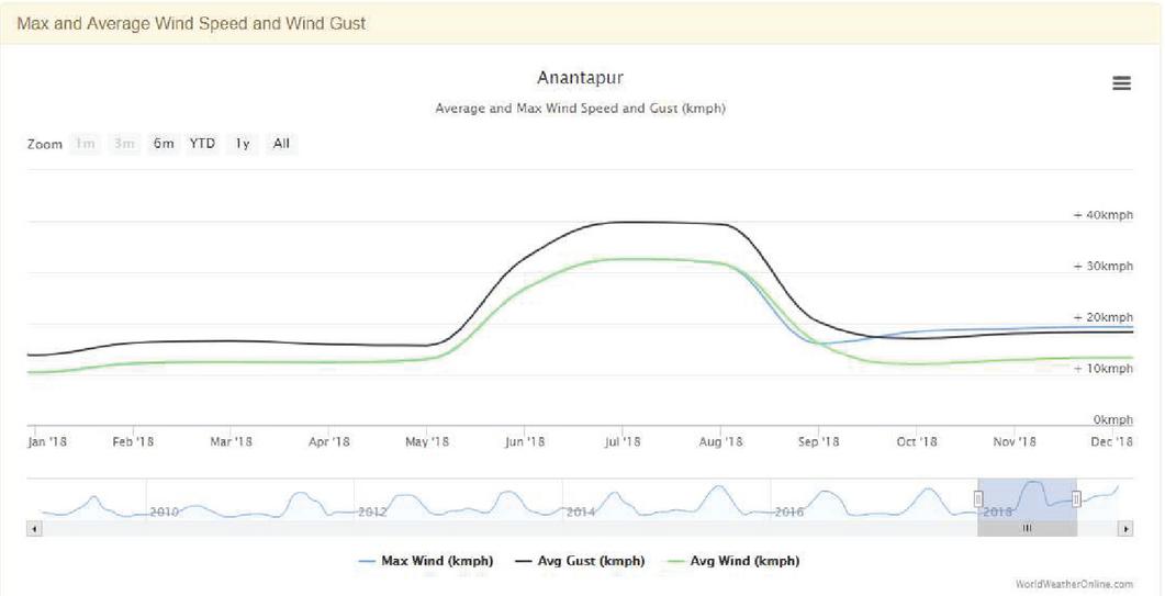
Figure 1 Maximum, minimum and average wind speed at Anantapuram, Andhra Pradesh.

The latitude and longitude of the Anantapuram location are 14.55 N and 77.75 E respectively. WTGU specifications are taken from [35] for the proposed method. Figure 1 shows the complete one-year monthly average wind speed along with the minimum and maximum wind speed. The annual average wind speed is 5.16 m/s (18.59 km/h) based on an average of the one-year average monthly wind speed. The maximum power output from the WTGU is obtained from Equation (23). The output power of one WTGU is 96.67 kW. The WTGU value is fixed for test systems testing in this paper, and the number WTGU placed in single or multiple locations will be varied depending on the test system’s optimal solution.

8 EDS with WTGUs Placement

The WTGUs are connected to EDS, and its static model has been used to analyze load flow in the distribution system [24]. Consider an equivalent circuit model of the standard radial distribution system branch between nodes p and q, as illustrated in Figure 2, which includes WTGUs at the q node.

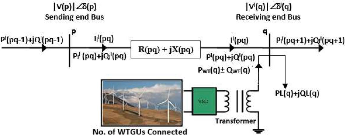
Figure 2 EDS equivalent model of a branch pq with WTGUs.

In Figure 2, the voltage magnitudes and phase angles of node p and q with WTGUs are $|V(p)|\mathrm{\angle }\delta (p)$ and $|V^1(q)|\mathrm{\angle }{\delta }^1(q)$, respectively, and power flowing along the line $pq$ is $P^1(pq)+j{Q}^1(pq)$ and $P_1^1(pq)+j{Q}_1^1(pq)$ at receiving end and sending end nodes changes with WTGUs.

9 Constraints for MOPI Optimization for WTGUs Placement

The following equality and inequality constraints are considered for WTGUs planning and optimization in EDS to minimize the generalized MOPI objective function in order to keep the operating condition within the limit.

9.1 Equality Constraints

9.1.1 Active power conservation limits including WTGUs

The algebraic sum of all active power including active power branch losses and produced active power from the WTGUs over the complete EDS should be equal to zero

$P_{s/s}={\displaystyle \sum _{q=1}^{nd}}PL(q)+{\displaystyle \sum _{pq=1}^{br}}{P}_{loss}(pq)-{\displaystyle \sum _{w=1}^{nwt}}{N}_{WT}(w)*P_{WT}$

(25)

where

${\displaystyle \sum _{w=1}^{nwt}}{N}_{WT}(w)*P_{WT}\mathit{\hspace{1em}}\text{is total kW injected capacity of WTGUs in EDS}$

nwt is the number of WTGUs.

9.1.2 Reactive power conservation limits including WTGUs [36]

The algebraic sum of all reactive power including reactive power branch losses and produced reactive power or absorbed reactive power from the WTGUs over the complete EDS should be equal to zero

$Q_{s/s}$	$={\displaystyle \sum _{q=1}^{nd}}QL(q)+{\displaystyle \sum _{pq=1}^{br}}{Q}_{loss}(pq)$
	$\mathrm{\hspace{1em}}\pm {\displaystyle \sum _{w=1}^{nwt}}{N}_{WT}(w)*P_{WT}*\sqrt{{\displaystyle \frac{1-co{s}^2\theta }{\cos \theta }}}$	(26)

where

${\displaystyle \sum _{w=1}^{nwt}}{N}_{WT}(w)*P_{WT}*\sqrt{{\displaystyle \frac{1-co{s}^2\theta }{\cos \theta }}}$

is total KVAr injected capacity of WTGUs

$cos\theta$ is the power factor of WTGUs.

9.2 Inequality Constraints

9.2.1 Injected active power for WTGUs

The injected active power by all WTGUs at various candidate nodes should be within their minimum and maximum limits.

$P_{WT}^{min}\le {\displaystyle \sum _{p=1}^{nwt}}{N}_{WT}(p)*P_{WT}\le P_{WT}^{max}$

(27)

where $P_{WT}^{min}$ is minimum WTGUs value of real power i.e. single WTGU value

$$P_{WT}^{max}\text{is total active load available in EDS i.e.}\mathit{\hspace{1em}}\sum _{q=1}^{nd}PL(q)$$

9.2.2 Injected reactive power of WTGUs

The injected reactive power by all WTGUs at various candidate nodes should be within their minimum and maximum limits.

$Q_{WT}^{min}\le {\displaystyle \sum _{w=1}^{nwt}}{N}_{WT}(w)*P_{WT}*\sqrt{{\displaystyle \frac{1-co{s}^2\theta }{\cos \theta }}}\le Q_{WT}^{max}$

(28)

where $Q_{WT}^{min}$ is minimum WTGUs value of reactive power i.e. single WTGU value

$Q_{WT}^{max}\text{is total reactive load available in EDS i.e.}\mathit{\hspace{1em}}{\displaystyle \sum _{q=1}^{nd}}QL(q)$

9.2.3 Line thermal limit [36]

For thermal and stability measure, the constraint of maximum power flow in the branch is needed to measure. The carrying power capacity of the branch is represented by MVA limit ($S(pq)$) throw any branch pq must within the maximum thermal capacity ($S^{max}(pq)$) of the branch

$$S(pq)\le S^{max}(pq)$$

(29)

10 Flow Chart for WTGUs Placement and Sizing Using ITLBO Algorithm

ITLBO is utilized to minimize the MOPI objective function, namely Equation (9), in order to solve the single and multiple optimal positions and related position sizes of the WTGUs allocation problem in EDS. The proposed method flow chart is shown in Figure 3. ITLBO algorithm parameters (such as generation number, population size (number of students), number of subjects and teachers), constraints, and EDS specifications (including node and line data) can all be considered ITLBO input at first. The WTGUs position can be any integer between 2 to the system’s maximum number of nodes (because 1 is a substation).

The minimum size of the corresponding locations is one WTGU for WTGUs placement, and the maximum size is less than or equal to the total active power load of EDS, respectively. The objective function variables are the WTGUs position and WTGUs reactive power size. Initializing the locations and sizes of the WTGUs in terms of the ITLBO subjects is shown in Figure 3. The MOPI objective function evaluation is done for a given population size using EDS load flow and calculates EDS performance indices by checking equality and inequality constraints. Hence, the ITLBO can be ranked to determine the global best solution (i.e., chief teacher), and ITLBO proceeds further to identify the number of teachers, learners under each group. Evaluate the teaching phase and learner phase for the next iteration as shown in Figure 3. The convergence criteria is set to the number of generations or when the present global solution does not change for a defined number of iterations.

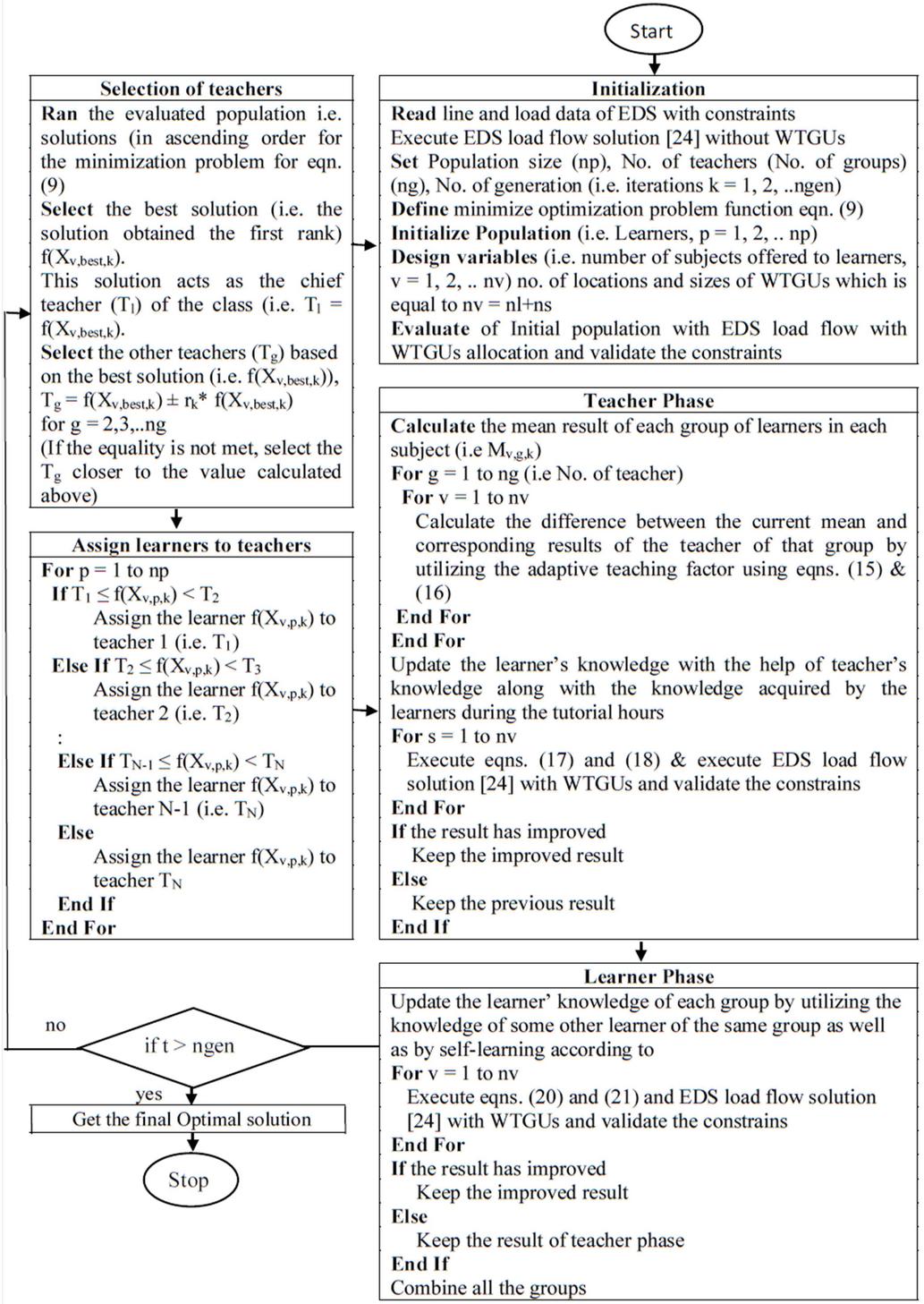
Figure 3 Flow chart for WTGUs Placement and Sizing using ITLBO.

11 Results and Analysis

The standard 33 node EDS [37] consists of 32 branches and 33 nodes with a total load demand of 3715 kW and 2300 kVAr. The system operates at a base voltage of 12.66 KV and a base power of 100 MVA. The active and reactive power losses without any DGs (without WTGUs) in the EDS are 210.98 kW and 143.12 kVAr respectively, with a minimum voltage of 0.90378 p.u. in 33 node test system.

The MOPI optimization using ITLBO is performed on the 33 node EDS for WTGUs placement with power factor (pf) unity, 0.95 lead and 0.95 lag at single and multiple locations, respectively via flow chart shown in Figure 3. The number of population size is taken as 50 and the number of subjects is twice the number of locations to solve the proposed ITLBO method. The locations and sizes (kW) of WTGUs, APL in kW, RPL in kVAr, $|$V$|$ min in p.u., VSImin in p.u., PLAMmax in kW and LLMmin in MW for the proposed MOPI optimization using ITLBO for WTGUs placement with pf unity, 0.95 lead and 0.95 lag at single and multiple locations and also presented the existing methods for comparison in Table 1. From the Table 1, the problem method has reduced the total real and reactive power losses, enhanced the minimum voltage, minimum VSI & line loadability and reduced the consumer loss allocation for 33 node EDS with WTGUs placement at single and multiple locations. The number of WTGUs (1 WTGU $=$ 96.67 kW) placed (with pf unity, 0.95 lead, 0.95 lag) at one, two, and three locations are 16 WTGUs, 19 WTGUs, and 30 WTGUs, respectively and it has been observed that WTGUs placement with pf 0.95 lead has given better EDS performance results compared with WTGUs placement with pf unity and 0.95 lag at one, two, and three locations respectively.

From Table 1, it can be noticed that the active and reactive power loss has been reduced to 90.73 kW, 50.40 kW & 30.90 kW, and 66.19 kVAr, 34.40 kVAr & 22.52 kVAr respectively for WTGUs placement (with pf of 0.95 lead) at single, two, and three locations from 210.98 kW and 143.12 kVAr respectively by using the proposed MOPI optimization using the ITLBO based method. The power loss reduction is slightly higher compared with existing methods for WTGUs placement at single, two, and three locations, respectively as compared with the base case in 33 node EDS. Better improvement has observed to increase the minimum node voltage from 0.90378 p.u to 0.93239 p.u., 0.97498 p.u. & 0.97967 p.u., increase the minimum VSI from 0.66901 p.u to 0.75770 p.u., 0.90459 p.u. & 0.92212 p.u., decrease the VDI from 0.32299 to with the voltage limits, increase the minimum LLM from 15.64 MW to 16.65 MW, 18.65 MW and 18.83 MW, and decrease the maximum customer loss allocation from 22.61 to 10.06 kW, 9.45 kW and 6.63 kW with WTGUs placement with pf 0.95 lead at one, two and three locations respectively from Table 1.

Table 1 Summary of the results to observe the performance of WTGUs placement at different locations in the 33 node EDS

		WTGU size			Total	Total	${|\mathrm{V}|}_{\min }$		VSI${}_{\min }$	LLM${}_{\min }$	PLAM${}_{\max }$
Case	Method	in kW (Location)	Power Factor		APL (kW)	RPL (kVAr)	(p.u)	VDI	(p.u.)	(MW)	(kW)
Base Case	–	–	–	210.97	143.12	0.90378	0.32299	0.66901	15.64	22.61
WTGUs	Proposed	1546.72 (30)	Unity	125.15	89.35	0.92730	zero	0.74132	16.47	10.93
at 1	Method		0.95 lead	90.73	66.19	0.93239	zero	0.75770	16.65	10.06
Location			0.95 lag	178.34	125.65	0.92188	0.20706	0.72415	16.27	17.61
WTGUs	Proposed	773.36 (14)	Unity	87.96	60.07	0.96441	zero	0.86603	18.61	11.44
at 2	Method	1063.37 (30)	0.95 lead	50.40	34.40	0.97498	zero	0.90459	18.65	9.45
Locations			0.95 lag	147.90	101.69	0.95076	zero	0.81912	18.03	17.55
WTGUs	Proposed	773.36 (14)	Unity	72.80	50.70	0.96849	zero	0.88076	18.77	10.67
at 3	Method	1063.37 (24)	0.95 lead	30.90	22.52	0.97967	zero	0.92212	18.83	6.63
Locations		1063.37 (30)	0.95 lag	142.95	98.30	0.95420	zero	0.83103	18.16	17.32
	QOTLBO [17]	600 (14)	Unity	90.94	62.03	0.94919	zero	0.81372	17.95	29.21
		598 (25)	0.86 (14)	lead	34.78	24.34	0.96899	zero	0.88369	18.64	8.62
		934 (30)	0.71 (25)	lag	230.42	157.97	0.92754	zero	0.74207	17.15	54.84
			0.70 (30)

From the above discussion, it can be concluded that the MOPI optimization using ITLBO based methodology shows better performance to improve EDS overall performance compared with existing methods, and existing methods concentrate only on reducing the losses in the EDS. The proposed method has reduced the losses in compromise with existing methods, but EDS performance improvement wise, the proposed method has shown better performance with respect to enhancing the minimum voltage, improve the voltage stability, reducing the VDI, improving the LLM, and reducing the loss burden of consumers. With the new generalized MOPI function, EDS performance has been handled in a better way with the results presented in Table 1 with WTGUs placement at one, two, and three locations.

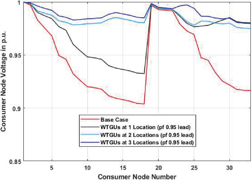
Figure 4 Voltage profile improvement for WTGUs placement at different locations in the 33 node EDS.

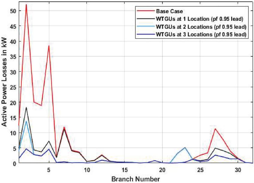
Figure 5 Active power losses for WTGUs placement at different locations in the 33 node EDS.

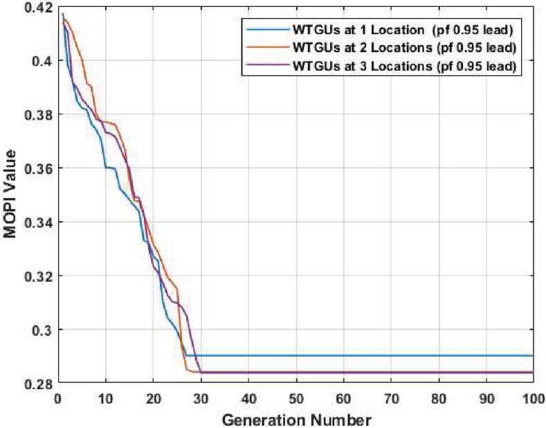
Figure 6 ITLBO convergence with MOPI objective function for WTGUs placement at different locations in the 33 node EDS.

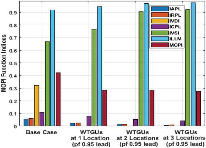
Figure 7 Analysis of MOPI Function Indices for WTGUs placement at different locations in the 33 node EDS.

Figures 4 and 5 show the enhancement in node voltage profile and active power loss reduction, under WTGUs placement at one, two and three locations in 33 node EDS. Figure 6 shows the convergence of the MOPI optimization using ITLBO and most of the cases with the WTGUs placements with pf 0.95 lead at different locations, the solution is to get the optimal value before 28 iterations for 33-node EDS. The good optimal solution gets based on the objective function with a global solution. The number of iterations for convergence has increased as increasing the complexity of the problem. Figure 7 has shown the MOPI function indices values for different WTGUs placement in 33 node EDS. From Figure 7 it has observed that IAPL, IRPL, IVDL & ICPL are decreased whereas IVSI & ILLM are increased and MOPI has decreased for getting the best performance of EDS from the base case to WTGUs placement with pf 0.95 lead at different locations in 33 node EDS.

12 Conclusions

In this paper, the utilization of the ITLBO procedure for solving WTGUs (with different pfs) placement at single and multiple locations as well as number of WTGUs problem for minimizing the EDS MOPI objective function has been proposed independently. ITLBO has been used to search for the optimal location and size of WTGUs at a different number of locations among a large number of combinations by optimizing the minimization MOPI objective function. The proposed MOPI optimization using ITLBO based method is applied to 33 node EDS with WTGUs(with different pfs) placed at one, two, and three locations. The results were compared and discussed with other existing methods and also discussed the effectiveness of the proposed method. The attained results have been shown that the proposed approach reduces the power loss slightly more than the existing methods and also shown the greater performance in improving the node voltage profile by reducing the VDI, enhanced minimum VSI, enhanced the minimum LLM and reduced the consumer loss allocation in the EDS with independent placement of WTGUs (with different pfs). WTGUs placement with pf 0.95 (lead) has been shown to have high EDS performance and overall EDS performance has been improved with individual placement of WTGUs (with different pfs).

References

[1] T. Ackermann, G. Andersson, and L. Soder, “Distributed generation: a definition”, Electric power systems research, Vol. 57, No. 3, Apr. 2001, pp. 195–204.

[2] P.S. Georgilakis and N.D. Hatziargyriou, “Optimal distributed generation placement in power distribution networks: Models, methods, and future research”, IEEE Transactions on Power Systems, Vol. 28, No. 3, Aug. 2013, pp. 3420–3428.

[3] A. Keane and M. O’Malley, “Optimal allocation of embedded generation on distribution networks”, IEEE Transactions on Power Systems Vol. 20, No. 3, Aug. 2005, 1640–1646.

[4] N. Acharya, P. Mahat and N. Mithulananthan, “An analytical approach for dg allocation in primary distribution network”, International Journal of Electrical Power and Energy Systems Vol. 28, No. 10, Dec. 2006, pp. 669–678.

[5] C.L. Borges and D.M. Falcao, “Optimal distributed generation allocation for reliability, losses, and voltage improvement”, International Journal of Electrical Power and Energy Systems, Vol. 28, No. 6, Jul. 2000, pp. 413–420.

[6] G.P. Harrison, A. Piccolo, P. Siano and A.R. Wallace, “Hybrid GA and OPF evaluation of network capacity for distributed generation connections”, Electric Power Systems Research, Vol. 78, No. 3, Mar. 2008, pp. 392–398.

[7] R. Jabr and B. Pal, “Ordinal optimisation approach for locating and sizing of distributed generation”, IET Generation, Transmission and Distribution, Vol. 3, No. 8, Aug. 2009, pp. 713–723.

[8] T. Shukla, S. Singh, V. Srinivasarao and K. Naik, “Optimal sizing of distributed generation placed on radial distribution systems”, Electric Power Components and Systems, Vol. 38, No. 3, Jan. 2010, pp. 260–274

[9] N. Khalesi, N. Rezaei and M.-R. Haghifam, “DG allocation with application of Dynamic Programming for loss reduction and Reliability Improvement”, International Journal of Electrical Power and Energy Systems, Vol. 33, No. 2, Feb. 2011, pp. 288–295.

[10] A. El-Zonkoly, “Optimal placement of multi-distributed generation units including different load models using particle swarm optimization”, Swarm and Evolutionary Computation, Vol. 1, No. 1, Aug. 2011, pp. 50–59.

[11] F.S. Abu-Mouti and M. El-Hawary, “Optimal distributed generation allocation and sizing in distribution systems via artificial bee colony algorithm”, IEEE transactions on power delivery, Vol. 26, No. 4, Oct. 2011, pp. 2090–2101.

[12] M.H. Moradi and M. Abedini, “A combination of genetic algorithm and par- ticle swarm optimization for optimal dg location and sizing in distribution systems”, International Journal of Electrical Power & Energy Systems, Vol. 34, No. 1, Jan. 2012, pp. 66–74.

[13] K. Nekooei, M.M. Farsangi, H. Nezamabadi-Pour and K.Y. Lee, “An improved multi-objective harmony search for optimal placement of dgs in distribution systems”, IEEE Transactions on smart grid, Vol. 4, No. 1, Feb. 2013, pp. 557–567.

[14] M. Aman, G. Jasmon, A. Bakar and H. Mokhlis, “A new approach for opti- mum dg placement and sizing based on voltage stability maximization and minimization of power losses”, Energy Conversion and Management, Vol. 70, Jun. 2013, pp. 202–210.

[15] S. Kansal, V. Kumar and B. Tyagi, “Optimal placement of different type of dg sources in distribution networks”, International Journal of Electrical Power & Energy Systems Vol. 53, Dec. 2013, pp. 752–760.

[16] R. Al Abri, E.F. El-Saadany and Y.M. Atwa, “Optimal placement and sizing method to improve the voltage stability margin in a distribution system using distributed generation”, IEEE transactions on power systems, Vol. 28, No. 1, Feb. 2013, pp. 326–334.

[17] S. Sultana and P.K. Roy, “Multi-objective quasi-oppositional teaching learning-based optimization for optimal location of distributed generator in radial distribution systems”, International Journal of Electrical Power & Energy Systems, Vol. 63, Dec. 2014, pp. 534–545.

[18] A.M. Imran and M. Kowsalya, “Optimal size and siting of multiple distributed generators in distribution system using bacterial foraging optimization”, Swarm and Evolutionary computation, Vol. 15, Apr. 2015, pp. 58–65.

[19] C. Yammani, S. Maheswarapu and M.S. Kumari, “Optimal placement and sizing of ders with load variations using bat algorithm”, Arabian Journal for Science and Engineering, Vol. 39, No. 6, Jun. 2014, 4891–4899.

[20] M. Kefayat, A.L. Ara and S.N. Niaki, “A hybrid of ant colony optimization and artificial bee colony algorithm for probabilistic optimal placement and sizing of distributed energy resources”, Energy Conversion and Management, Vol. 92, Mar. 2015, pp. 149–161.

[21] N. Mohandas, R. Balamurugan and L. Lakshminarasimman, “Optimal location and sizing of real power dg units to improve the voltage stability in the distribution system using abc algorithm united with chaos”, International Journal of Electrical Power & Energy Systems, Vol. 66, Mar. 2015, pp. 41–52.

[22] E. Ali, S.A. Elazim and A. Abdelaziz, “Ant lion optimization algorithm for optimal location and sizing of renewable distributed generations”, Renewable Energy, Vol. 101, Feb. 2017, pp. 1311–1324.

[23] I.A. Quadri, S. Bhowmick and D. Joshi, “A comprehensive technique for optimal allocation of distributed energy resources in radial distribution systems”, Applied Energy, Vol. 211, Feb. 2018, 1245–1260.

[24] T. Ramana, V. Ganesh and S. Sivanagaraju, “Simple and Fast Load Flow Solution for Electrical Power Distribution Systems”, International Journal on Electrical Engineering and Informatics, Vol. 5, No. 3, September 2013, pp. 245–255.

[25] N.S. Rau, and Y.-h. Wan, “Optimum location of resources in distributed planning”, IEEE Transactions on Power Systems, Vol. 9, No. 4, Nov. 1994, pp. 2014–2020.

[26] T. Ramana, V. Ganesh, S. Sivanagaraju and K Nagaraju, “Customer Loss Allocation Reduction using Optimal Conductor Selection in Electrical Distribution System”, Emerging Trends in Electrical, Communications, and Information Technologies, Proceedings of ICECIT-2018, Electrical and Electronics Engineering, Lecture Notes in Electrical Engineering Series by Springer, pp. 369–379, 2019.

[27] M. Chakravorty and D. Das, “Voltage stability analysis of radial distribution networks,” International Journal of Electrical Power and Energy Systems, Vol. 23, No. 2, Feb, 2001, pp. 129–135.

[28] J. Yu, W. Li and W. Yan, “Letter to the Editor: A New Line Loadability Index for Radial Distribution Systems”, Electric Power Components and Systems, Vol. 36, No. 11, Oct. 2008, pp. 1245–1252.

[29] R.V. Rao, V.J. Savsani and D.P. Vakharia, “Teaching-learning-based optimization: a novel method for constrained mechanical design optimization problems”, Computer-Aided Design, Vol. 43, No. 3, Mar. 2011, pp. 303–315.

[30] F. Cus and J. Balic, “Optimization of cutting process by GA approach”, Robotics and Computer Integrated Manufacturing, Vol. 19, No. 1/2, Feb. 2003, pp. 113–121.

[31] J. Kennedy and R.C. Eberhart, “Particle swarm optimization”, In: Proceedings of ICNN’95 – International Conference on Neural Networks, 27 Nov.–1 Dec. 1995, pp. 1942–1948.

[32] R.V. Rao and V. Patel, “An improved teaching-learning-based optimization algorithm for solving unconstrained optimization problems”, Scientia Iranica, Vol. 20, No. 3, Jun. 2013, pp. 710–720.

[33] K.C. Divya and P.S.N. Rao, “Models for wind turbine generating systems and their application in load flow studies”, Electrical Power System Research, Vol. 76, No. 9/10, Jun. 2006, pp. 844–856.

[34] https://www.worldweatheronline.com/lang/en-in/anantapur-weather-averages/andhra-pradesh/in.aspx

[35] Wei Z, Hongxing Y, Lin L, Zhaohong F. “Optimum design of hybrid solar–wind–diesel power generation system using genetic algorithm”, HKIE Transactions, Vol. 14, No. 4, 2007, pp. 82–89.

[36] V. Kumar, R. Kumar, I. Gupta and H.O. Gupta, “DG Integrated approach for service restoration under cold load pickup”, IEEE Transactions Power Delivery, Vol. 25, No. 1, Jan. 2010, pp. 398–406.

[37] N.C. Sahoo and K. Prasad, “A fuzzy genetic approach for network reconfiguration to enhance voltage stability in radial distribution systems”, Energy Conversion and Management, Vol. 47, No. 18/19, Nov. 2006, pp. 3288–3306.

Biographies

Thiruveedula Ramana received the bachelor’s degree in electrical and electronics engineering from JNT University, Hyderabad in 2020, the master’s degree in power and industrial drives from JNT University, Kakinada in 2010, and the philosophy of doctorate degree in Electrical Engineering from JNT University, Anantapur in 2019, respectively. He is currently working as an Associate Manager at the Global Delivery India Centre, DXC Technology India Private Limited, Bangalore, India. His research areas include distribution system automation, renewable energy sources, FACTs, power system analysis. He has been serving as a reviewer for many highly-respected journals.

G. Nageswara Reddy, is Assistant professor in the department of Electrical and Electronics Engineering, YSR Engineering college of Yogi Vemana University, Proddatur, A.P., India. He received B.Tech, M.Tech, and Ph.D in Electrical and Electronics Engineering from, Jawaharlal Nehru Technological University Hyderabad, Hyderabad. His interests include, Power System Analysis including FACTS devices, Optimization Techniques and Power System Operation and Control.

Distributed Generation & Alternative Energy Journal, Vol. 37_5, 1637–1664.
doi: 10.13052/dgaej2156-3306.37514
© 2022 River Publishers

Abstract

1 Introduction

2 Formation of Multi-objective Problem with Different EDS Performance Indices

2.1 Index for Active Power losses (IAPL) and Index for Reactive Power Losses (IRPL) Based on Available Load

2.2 Index for Node Voltage Deviation (IVDI)

2.3 Consumer Loss Allocation Index Based on Total APL (ICPL)

2.4 Index for VSI (IVSI)

2.5 Index for LLM (ILLM)

3 General Multi-Objective Optimization Problem

4 TLBO Algorithm

4.1 Teacher Phase

4.2 Learner Phase

5 Improved TLBO Algorithm

5.1 Number of Teacher

5.2 Adaptive Teaching Factor

5.3 Learning Through the Tutorial

5.4 Self-motivated Learning

6 Performance Model of WTGU

7 Size of the WTGU

8 EDS with WTGUs Placement

9 Constraints for MOPI Optimization for WTGUs Placement

9.1 Equality Constraints

9.1.1 Active power conservation limits including WTGUs

9.1.2 Reactive power conservation limits including WTGUs [36]

9.2 Inequality Constraints

9.2.1 Injected active power for WTGUs

9.2.2 Injected reactive power of WTGUs

9.2.3 Line thermal limit [36]

10 Flow Chart for WTGUs Placement and Sizing Using ITLBO Algorithm

11 Results and Analysis

12 Conclusions

References

Biographies