Anomaly Detection of Smart Grid Equipment Using Machine Learning Applications

Arun Sekar Rajasekaran^1,*, P. Kalyanchakravarthi¹ and Partha Sarathi Subudhi^{2, 3}

¹Department of Electronics and Communication Engineering, GMR Institute of Technology, GMR Nagar, Rajam – 532 127, Andhra Pradesh, India
²Department of Electrical Engineering, Bajaj Institute of Technology (BIT), Wardha, Maharashtra, India
³Department of Electrical and Electronics Engineering, Faculty of Engineering and Architecture, Nisantasi University, Istanbul, Turkey
E-mail: arunsekar.r@gmrit.edu.in; rarunsekar007@gmail.com; kalyanchakravarthi.p@gmrit.edu.in; partharesearch.vit@gmail.com
*Corresponding Author

Received 22 February 2022; Accepted 03 May 2022; Publication 24 June 2022

Abstract

Many application systems in today’s smart grid network comprise a variety of middleware components, such as vibrating or spinning electrical equipment, data bases, storage, caches, and identification services, among others. Each component is a discrete bundle of physical or virtual computers that will generate a large amount of data in the form of logs and metrics, and failure of these high-vibrating machines will result in the system’s entire shutdown. As a result, the condition monitoring system for this smart grid equipment is more dependable and efficient in predicting the machine’s health ahead of time. To analyze the data and derive any inferences for future analysis and anomaly detection, we’ll need a separate system, which will take longer to handle data given by each component and will demand additional processing resources. As a result, in this chapter, machine learning methods are used to identify abnormalities or condition monitoring for smart grid equipment and machines. Here, we used two separate methods: multivariate statistical analysis by calculating Mob distance and auto encoders, which is an artificial neural network approach. Furthermore, the findings demonstrate that these apps are effective in identifying anomaly ahead of time, i.e. before a few days.

Keywords: Anomaly, multivariate statistical analysis, principal component analysis, condition monitoring.

1 Introduction

The basic purpose of popular ideas like as digital transformation, digitalization, and Industry 4.0 is to use data and technology to improve productivity and efficiency. The relativity and connectedness of data across middleware components and sensors in application systems results in an abundance of accumulated data. The main issue is to figure out how to handle this massive volume of data and extract just useful facts. As a consequence of this pre-processing, costs will be reduced and capacity will be increased. The latest trends of data analytics and machine learning come into play to accomplish these advantages. Anomaly detection is one of the applications of machine learning. An anomaly is a deviation from the typical flow of a time series pattern. Consider the following scenario: we wanted to track traffic volume every day, so we produced a graph of time vs. traffic volume.

Figure 1 Traffic volume (KPI) vs time series plot in a certain area.

The plot of traffic volume vs. time is shown in Figure 1. Each cycle represents a day’s worth of traffic. On the first two days, traffic volume is typical, but on the third day, it is abnormally low, and this is referred to as an anomaly. On regular days, a huge number of police officers and other equipment in that region are necessary to regulate traffic. However, if the same number of police officers are present on the third day, it is a waste of manpower with little traffic. If they were in another location, traffic management in that region may be beneficial. So, if we see that there won’t be significant third-day traffic on the second day or within a few days, we’ll take action. The control room will then take the required safeguards by dispatching police officers to another location. In this case, we may use machine learning to discover the abnormality. We will first anticipate the time series pattern for tomorrow’s traffic volume, and then calculate the difference between the projected and actual time series patterns, which will assist us in quickly finding anomaly and reporting them to the network control centre. Furthermore, they will choose the best remedy for this abnormality. We’ll use machine learning for predicting, which will need training data for the ML model, which will include time series against traffic volume from previous weeks. In addition, we must provide seasonal data to the ML model by merging data from the previous several weeks as training data. So, in real-time circumstances, detecting this abnormality might save us a lot of time, electricity, and other resources. Furthermore, in the event of any machinery or equipment that is continually operating and running, any internal portion of it may suddenly fail on one day, making it impossible to replace that part on the same day. So, if we discover the abnormality ahead of time by drawing a graph between the parameter that indicates the machine’s performance vs time, we can take the appropriate action (by replacing/repairing) on that machine before it breaks down. Machine learning model is required for anomaly detection system to analyze the data and derive any inferences for future analysis. Moreover, Machine learning model permit to systematize anomaly detection and make it more operative, specifically when large datasets are involved.

Anomaly

The word “anomaly” has a variety of mathematical and formal meanings. An outlier is a value that falls outside of specified limitations or thresholds in this time series and statistical concept. Furthermore, the term anomaly may be used to specific time points or longer time periods when a constantly aberrant behaviour of time series is expected. Currently, an anomaly is defined as any pattern of a time series value that differs from the regular signal pattern during a time in our research. Furthermore, the detection system needs a machine learning model that is trained on training data to be able to categorize distinct patterns, define, and anticipate a pattern, as well as the estimated difference to a threshold limit. The anomaly score is the magnitude of this discrepancy, and its behaviour causes the threshold border to be calculated and defined. Anomaly may be identified in a variety of ways, including signal spikes or sudden decreases, as well as longer, more continuous development spans or short-term oscillations. A phase that is aberrant based on the situational context, the analyst’s interpretation, and domain expertise. Other related metrics and dependent components must be considered in the situational context. Analysts with access to manage, identify, and verify anomaly, such as production support engineers, should be on the lookout for them. The following are some instances of anomaly in various settings.

In real-time circumstances, the anomaly in the three images above are instances of anomaly in any series pattern. Anomaly/abnormal instances are shown by red coloured values in each plot, whereas typical behaviour/pattern is represented by green coloured values.

Anomaly Detection: It’s also known as outlier detection [1, 2], which is the identification of rare occurrences, things, or data points that differ significantly from the rest of the data. Anomaly data is often linked to some form of anomaly or uncommon occurrence, such as bank fraud, medical issues, equipment failure, and so on. To determine if a particular test data point is an anomaly, we must first evaluate past data from that equipment. Data visualization, i.e., generating a plot between any two variables and viewing it and determining which data point is out of the distribution, is one of the greatest ways to spot an anomaly.

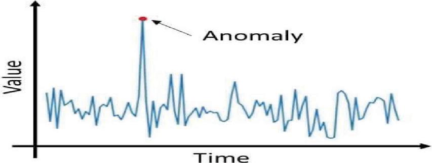
Figure 2 Detecting of Anomaly when two variables are there.

Figure 2 depicts the detection of anomaly when two variables are present. If we look at the relative distribution between X and Y in the case of data with two dimensions (i.e. with two variables X and Y), we may readily detect data points that are outside the normal distribution. However, identifying outliers from individual variable distributions (right side figures of the above plot) at a time is challenging. As a result, by combining the two variables X and Y, we may easily notice the anomaly indicated above. However, transmitting data with more than 100 variables makes it tough and hard to identify an abnormality, which is often the case in real-time situations of anomaly detection. Some of the security related issues are discussed in the works [3–7].

The work is organised as follows. The problem statement is elucidated in Section 2. The strategies for detecting anomaly are discussed in Section 3. In Section 4, applications such as gear bearing failure detection are shown. Section 5 explains the simulation setup programmers, part 6 explains the findings summary, and Section 7 wraps up this paper.

2 Problem Statement

Any piece of spinning (pump, gearing) or non-rotating (valve, heat exchanger) equipment will have a plethora of internal pieces such as gearings, sensors, and so on. Furthermore, every machine will reach a point of failure, which is not a complete breakdown but rather a state in which the equipment is unable to perform or run as it would under normal circumstances. If this issue occurs unexpectedly, we will be unable to replace or repair it, and it will take additional time to return to its previous position. As a result, it should be identified in advance, i.e., sending a signal that indicates that some maintenance activity for the equipment is required so that it does not get sick. In other words, “condition monitoring” is nothing more than examining the “health status” of our equipment.

The most typical way to do condition monitoring is to look at each sensor measurement from the equipment and set a maximum and minimum threshold for it. The equipment is subsequently labelled unhealthy, and an indication is provided if the current value for any middleware sensor is not within certain limits at the time of testing. However, this approach of assigning limits to each sensor has the disadvantage of occasionally generating many false alarms. For example, if the current value exceeds the maximum value for one sensor and the current value is lower than the minimum value for the second sensor, the equipment is still healthy, but an alarm will be generated. There are also cases of missed alerts, in which the alarm is not issued even though the situation is dangerous. In the first scenario, it wastes time, effort, and equipment availability; in the second case, it is very troublesome and results in actual equipment damage. Consequently, all of the foregoing disadvantages arise from the same source: the state of complicated and large equipment cannot be determined only by analysing the condition of each sensor separately. To get a real signal regarding an equipment’s status, we should consider combining the numerous sensor data in the equipment. There are many supervised machine learning algorithms for best anomaly detection. Some of them includes kNN, LOF, SVM etc.

3 Anomaly Detection Techniques

Technique 1: Multivariate statistical analysis: –

This method combines two methods: dimensionality reduction using PCA (Principal component analysis) and calculating Mob distance.

(a) Dimensionality reduction using PCA:

As described in the data visualization section [8], dealing with data distribution with a larger number of variables is more difficult. So, we can apply dimensionality reduction to minimise complexity. It is the process of converting data from a high-dimensional space to a low-dimensional space while keeping some of the original data’s important representation and behaviors. Its intrinsic dimension is approximately same (It is the number of dimensions required in a minimal representation of the data). PCA (Principal component analysis) is one of the approaches that performs a linear mapping of the data to a lower-dimensional space for this dimension reduction. Furthermore, the variance of the data is highest here (expectation of the squared departure of a variable from its mean, which shows us how far a group of data points is spread out from the average value). This variance should be as high as feasible in order to preserve the most relevant section of the data distribution, which means Eigen vectors with the highest Eigen values are required. Furthermore, the Eigen vectors are calculated by creating the data’s covariance matrix. So that the Eigen vectors corresponding to the largest Eigen values may be utilized to reinterpret as much of the original data’s volatility as possible.

PCA:

PCA is the method of calculating main components and using them to transform the data’s foundation. First, the data is randomly dispersed, and the main components, which are two orthogonal vectors that tell us the direction and magnitude of data distribution, are calculated. These two vectors are also used to characterize the data distribution in a straightforward method. A series of direction vectors, where the nth vector is the direction of a line that reflects the direction of data distribution and is orthogonal to n-1 vectors, are the main components of a collection of data points in real space. To detect anomaly in a significant way, we first compute the p(x), which is the probability distribution from the data points, while processing a combination of data points, they will normally contain a specific distribution (for example, a Gaussian distribution), so to detect anomaly in a significant way, we first compute the p(x), which is the probability distribution from the data points. Then, using this p(x) as a reference, we’ll assess p(x) and the threshold ‘r’ when a test point ‘x’ comes in. If p(x) is smaller than ‘r,’ an anomaly is proclaimed.

The flow of applying principal component analysis is demonstrated in below Figure 3.

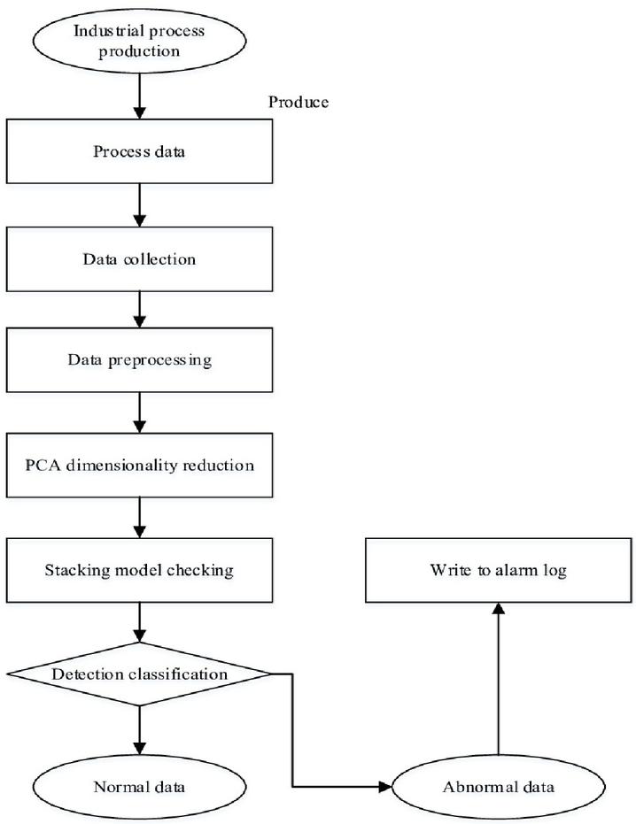
Figure 3 Flow of anomaly detection by using PCA.

(b) The Mob distance:

The computation of the Mahalanobis distance, often known as the Mob distance [9, 10], is another way of determining whether a point belongs to a distribution or not. The first step is to determine the sample sites’ centroid or centre of mass. If the test point is at the centre of mass, it is part of the set (normal pattern); otherwise, it is an anomaly. Furthermore, we must determine if the set is distributed across a greater or smaller range. So that we can determine the distance between the centre of mass and the threshold for checking for anomaly. The easiest way in this scenario is to compute the standard deviation (SD) of the distances between test points and the centroid, and then compare this to a typical distribution to determine if the data point belongs to the same distribution or is an anomaly. However, if the data is distributed in a non-spherical fashion, such as ellipsoidally, it is not relevant. In such situation, we must employ direction as a parameter to verify a test point, since in a spherical distribution, there would only be one radius of equal length from any point on the circumference to the centre, however in an ellipsoid, there will be two axes, one short and one longer. As a result, in the direction of the short axis, the test point should be closer to the centre, whereas in the direction of the long axis, the test point may be farther away from the centre. Calculating the covariance matrix of the samples is a mathematical approach to handle these types of elliptical data distributions. In addition, we must employ Mob distance (MD), which is the ratio of the distance between the test data point and the centre of mass to the width of the ellipsoid in the direction of the test point. Then, for each class, we’ll compute the covariance matrix (normal class & anomaly class). To generate the covariance matrix, we need training data that consists of normal data under typical operating circumstances. Then, using that covariance matrix, we’ll calculate a threshold and the MD to normal class. Only if the distance is greater than the expected limit will we classify a test data point as an anomaly.

In the proposed multivariate statistical analysis technique, PCA and mob distance methods are used for anomaly detection with same performance. Both the methods are combined together for better performance

Technique 2: Auto encoder Artificial neural network:

The use of an auto encoder network [11] is another way for detecting anomaly. It takes a similar approach to the first strategy, but with a few minor modifications. An auto encoder is a form of artificial neural network (ANN) that is inspired by biological neural networks. An artificial neural network (ANN) is a collection of linked units or nodes known as artificial neurons. It consists of an input layer, one or two hidden layers, and finally an output layer. And each layer has a number of nodes, each of which acts as a transfer function. The fundamental aim of an auto encoder is to learn (since it is an ML model, it must learn in an unsupervised way) a representation for a data set, which is generally used for dimension reduction. ANNs are used to develop a model that learns efficient data coding in an unsupervised manner.

It reduces dimensionality first, then reconstructs the original data representation as closely as feasible to the original input. Furthermore, this auto encoder is a feed forward neural network, which means that it goes directly from the input layer to the hidden layer and then to the output layer if there are no loops in the hidden layer (non-recursive), it only has one direction (forward), and the output layer and input layer both have the same number of nodes for the purpose of reconstructing its own inputs. The Auto encoder artificial neural network is seen in Figure 4.

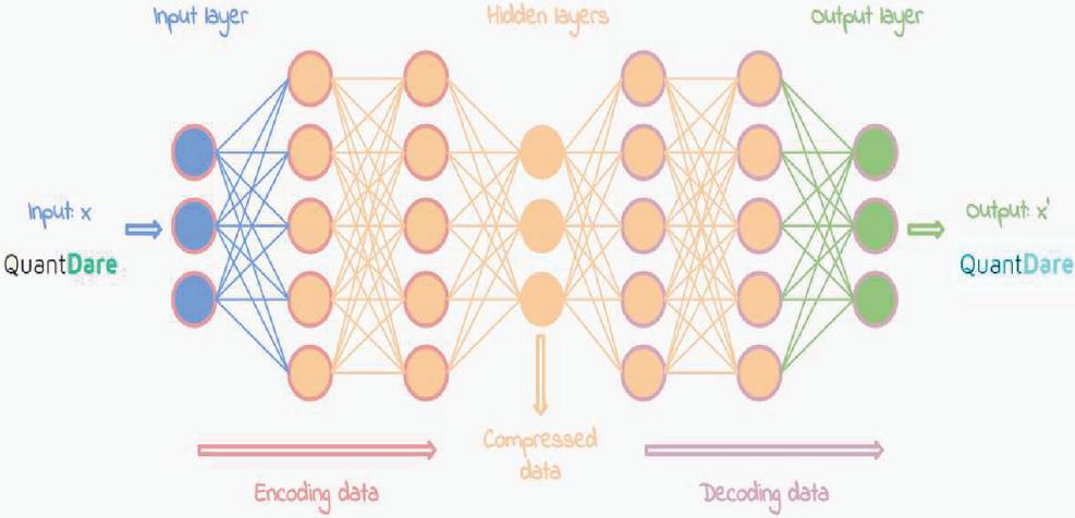
Figure 4 Auto encoder artificial neural network.

In general, we must handle data from sensor readings in equipment that may include a large number of variables. As with PCA, we will compress the larger number of variables to a lower-dimensional representation in auto encoder by taking into account correlations and interactions among the different variables. The distinction between auto encoder and PCA is that non-linear relationships between variables will be allowed.

The auto encoder model is then fed with a data set that represents the usual operating state, which is obtained by compressing the dimensionality first and then reconstructing the original data representation from the decreased dimensionality. The relationships and interactions between variables will be used to reduce the dimensions. All of this reduction and reconstruction will proceed without error for a typical data set, but if there is an anomaly, the original data will be reconstructed with a lot of errors. Because the presence of an anomaly in a dataset has an impact on the relationships between variables (changes in temperatures, pressures, vibrations etc.). So, when training the model with normal data, it will learn to identify which data is normal and which data is anomalous based on reconstruction loss, and the model will be able to detect anomaly and deliver an indicator if one is found. Furthermore, reconstruction error is detected by computing a probability distribution, such as the Mob distance, and comparing it to a threshold to determine if the data is normal or aberrant [12–14].

Both the techniques namely Multivariate statistical analysis and Auto encoder ANN are equally efficient and both the techniques are combined together for anomaly detection. Since both the methods detect the anomaly in less than 3 days, it is advantageous to use any of the techniques in detecting gear bearing failure in high speed wind turbine bearing.

4 Experimental Analysis

4.1 Applying ML Techniques as Condition Monitoring in Detecting Gear Bearing Failure in High-speed Wind Turbine Bearing

In this section, we’ll use the two strategies we mentioned before to create an application. We are monitoring the state of a high-speed wind turbine in a smart grid network that includes “Gear bearing”. It is a type of rolling-element bearing as shown in below Figure 5.

Figure 5 Gear bearing in an equipment.

The major goal is to identify gear bearing failure in advance and transmit a warning signal that allows for proactive steps (either replacement or repair). An equipment with four bearings was predicted to break down in this situation owing to constant load and continuous operating circumstances. We have three sets of data regarding four bearings, which comprise of vibration measurements during the lifespan of the bearings until failure, which occurred after 100 million cycles and was accompanied by a fracture in the exterior section, according to the presented data set. We will collect data for the first two days to train the model that depicts regular and “healthy” equipment since the machine will operate constantly until it breaks down. The third data set comprises data from when the bearing is about to fail, which is used to train the model as “anomalous data” since the vibrations may vary before the bearing fails. Let us now compare and contrast both bearing degradation strategies.

By using technique 1: (PCA $+$ Mob distance)

To determine if the data points are normal or abnormal, we will first do principal component analysis and then calculate the Mob distance (sign of bearing failure). In addition, Figure 6 shows the data distribution of Mob distance for training data indicating “healthy” equipment.

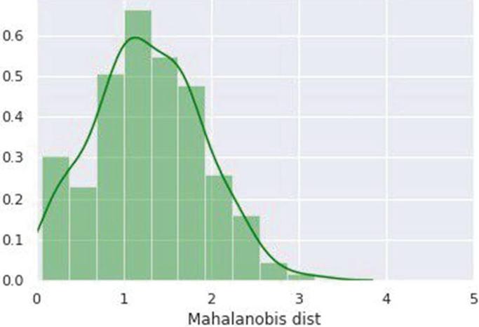
Figure 6 Diagram for MD for “healthy” equipment.

So, based on the aforementioned distribution, which represents “healthy” equipment, we can argue that if MD 3, the data set is normal; otherwise, it’s an oddity. The evaluation of this approach for detecting anomaly now entails computing MD for each data point in the test set and analysing with threshold. The MD distribution of all data points in the test data is shown in Figure 7.

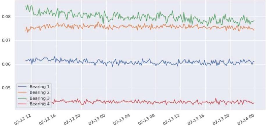
Figure 7 Predicting bearing failure using technique 1.

The green dots in the above distribution reflect the calculated Mob Distance for all locations, while the red line represents the threshold value. The bearing breakdown occurs near the conclusion of the data set, but the MD reaches the threshold before three days. As a result, we can diagnose bearing failure in less than three days. Let’s have a look at how the second approach detects anomaly in this scenario in advance.

By using technique 2: (Auto encoders)

We will utilise the reduction and reconstruction policies outlined in the technical section to calculate the reconstruction loss for the data set and then compute the probability distribution for that data set. First, it will compute the reconstruction loss for normal data, then determine the threshold.

Moreover, we can now establish a threshold of 0.25 from the above distribution of reconstruction loss for “healthy” equipment. It is an anomaly if the reconstruction loss for a data point is larger than 0.25. The assessment of this model on test data to identify anomaly is shown in Figure 8.

The blue dots in the distribution below represent the reconstruction loss for data points, while the red line represents the threshold level. Furthermore, bearing failure happened near the conclusion of the data set, as shown by the dotted lines. However, abnormal data began to show (threshold crossing) three days before the real breakdown.

Figure 8 Predicting bearing failure using technique 2.

Some real time scenarios where these anomaly detection techniques can be applied are as follows: Anomaly detection of gear bearing failure in high speed wind turbine bearing, detection of fraud in monetary businesses and detection of fault in engineering.

5 Result Summery

So, by combining these two strategies for anomaly detection, we may discover anomaly before they occur (in advance), and both techniques have been successful in detecting anomaly in the past (several days before only). So, in a real-time situation, we may utilize these strategies to transmit signals before a failure happens, allowing us to take any necessary preventative steps, such as repairing or replacing, saving both time and money. These anomaly detection techniques are sufficient for reducing better results. However, with changing technology and advancements in machine learning can be used for quicker anomaly detection as well as to track future breakdowns.

6 Conclusion

With the reduced cost of collecting data via sensors and increased connection between devices, it is becoming more vital to extract meaningful information from data. Finding patterns in vast amounts of data is the key growing characteristic of machine learning and statistics. Furthermore, utilizing two approaches (PCA $+$ Mob distance and auto encoders), data pre-processing and machine learning are used to identify anomalies in condition monitoring. These two methods were able to identify anomalies three days before the actual collapse. Furthermore, machine learning will evolve considerably further in the future than we can now envision. Furthermore, advanced machine learning may be utilized to discover anomalies even quicker in the future. Moreover, these techniques will help to track when the future breakdowns will occur.

References

[1] Karishma Pawar and Vahida Attar, “Deep learning approaches for video-based anomalous activity detection”, World Wide Web, vol. 22.2, pp. 571–601, 2019.

[2] Yuequan Bao et al., “Computer vision and deep learning-based data anomaly detection method for structural health monitoring”, Structural Health Monitoring, vol. 18.2, pp. 401–421, 2019.

[3] Iqbal, A., Rajasekaran, A. S., Nikhil, G. S., and Azees, M. A Secure and Decentralized Blockchain Based EV Energy Trading Model Using Smart Contract in V2G Network. IEEE Access, 9, 75761–75777, 2021.

[4] Rajasekaran, A. S., Azees, M., and Al-Turjman, F. A comprehensive survey on security issues in vehicle-to-grid networks. Journal of Control and Decision, 1–10, 2022.

[5] Leman Akoglu, Hanghang Tong and Danai Koutra, “Graph based anomaly detection and description: a survey”, Data mining and knowledge discovery, vol. 29.3, pp. 626–688, 2015.

[6] Arasan, A., Sadaiyandi, R., Al-Turjman, F., Rajasekaran, A. S., and Selvi Karuppuswamy, K. Computationally efficient and Secure Anonymous Authentication Scheme for Cloud Users. Personal and Ubiquitous Computing, Vol. 25, 2021.

[7] J. Subramani, A. Maria, A. S. Rajasekaran and F. Al-Turjman, “Lightweight Privacy and Confidentiality Preserving Anonymous Authentication Scheme for WBANs,” in IEEE Transactions on Industrial Informatics, vol. 18, no. 5, pp. 3484–3491, May 2022.

[8] Pang-Ning Tan, Michael Steinbach and Vipin Kumar, Introduction to data mining, Pearson Education India, 2016.

[9] Xiuyao Song et al., “Conditional anomaly detection”, IEEE Transactions on knowledge and Data Engineering, vol. 19.5, pp. 631–645, 2017.

[10] Nguyen Thanh Van and Tran Ngoc Thinh, “An anomaly-based network intrusion detection system using deep learning”, 2017 International Conference on System Science and Engineering (ICSSE). IEEE, 2017.

[11] Sarah M. Erfani et al., “High-dimensional and large-scale anomaly detection using a linear one-class SVM with deep learning”, Pattern Recognition, vol. 58, pp. 121–134, 2016.

[12] Lorenzo Fernández Maimó et al., “A self-adaptive deep learning-based system for anomaly detection in 5G networks”, IEEE Access, vol. 6, pp. 7700–7712, 2018.

[13] Ritesh K. Malaiya et al., “An empirical evaluation of deep learning for network anomaly detection”, 2018 International Conference on Computing Networking and Communications (ICNC). IEEE, 2018.

[14] Zahra Jadidi et al., “Flow-based anomaly detection using neural network optimized with GSA algorithm”, 2013 IEEE 33rd international conference on distributed computing systems workshops. IEEE, 2013.

Biographies

Arun Sekar Rajasekaran received his Bachelor’s degree in Electronics and Communication engineering from Sri Ramakrishna Engineering College in 2008 and his Master’s degree in VLSI Design in 2013 and his Doctorate of philosophy in Low Power VLSI design from Anna University, Chennai in 2019. He is currently working as an Assistant professor in the Department of Electronics and Communication Engineering at GMR Institute of Technology, Rajam, Andhra pradesh. He has nearly 12 years of Teaching experience. He had published more than 24 papers in International conferences and 23 reputed Indexed Journals namely, IEEE Transactions on Industrial informatics, Springer, (Microprocessor and microsystems, Computers and electrical engineering) Elsevier, IET communications, IEEE Access and Concurrency and computation (Wiley) publications. His areas of interest are Low power VLSI design, Network security, Blockchain, Body area networks and Image processing. He is a life member of ISTE, IETE, ISRD and IEANG.

P. Kalyanchakravarthi received the bachelor’s degree in Electronics and communication engineering from JNTU Hyderabad in 2007, the master’s degree in Electronics and communication engineering from NIT Rourkela in 2011, and currently pursuing the philosophy of doctorate degree in Electrical Engineering , NIT Rourkela. He is currently working as an Assistant Professor at the Department of Electronics and Communication Engineering, GMR Institute of Technology, Rajam, Andhrapradesh,India. His research areas include mobile security, deep learning, and social network analysis.

Partha Sarathi Subudhi, (M’15–SM’21, IEEE) completed his Bachelor of Technology in “Electrical Engineering” from Biju Patnaik University of Technology, Odisha, India in 2012 and Master of Technology in “Power Electronics and Drives” from Vellore Institute of Technology, Chennai, India in 2015. He then went on to join for a full-time Ph.D. with the School of Electrical Engineering (SELECT), Vellore Institute of Technology (VIT) from 2015 to 2020. Currently, he is an Adjunct Professor with the Department of Electrical and Electronics, Faculty of Engineering and Architectures, Nisantasi University, Istanbul, Turkey. He has been working as an Assistant Professor with the Department of Electrical Engineering, Bajaj Institute of Technology (BIT), Wardha, Maharashtra, India since 2021. He is an Editor of International Journal of Power and Energy Systems, Acta Press, and a Guest Editor of River Publisher. He is also managing editor of IEEE Educational Videos on Power Electronics. He is an active member of IEEE PELS. Dr. Subudhi is a member of the IEEE Technical Committee 9 (TC 9) on Wireless Power Transfer Systems. Recently, he got selected as a member of publication committee of IEEE PELS TC9. He is also a member of IEEE Technical Committee 12 (TC 12) on Energy Access and off Grid System. He is also a member of the IEEE PELS Educational Videos Committee. He is a life member of IEANG. He is also selected as a life member of ISTE, India. He had received best paper award in International Conference on Innovations & Discoveries in Science, Engineering and Technology 2018 (ICIDSET-18). His field of interest includes Power Electronics Converters, Wireless Power Transfer, Electric Vehicle Charger, Residential Nano Grid, Solar Power Generation System, Hybrid Converters, and their applications.

Distributed Generation & Alternative Energy Journal, Vol. 37_5, 1721–1738.
doi: 10.13052/dgaej2156-3306.37518
© 2022 River Publishers