Short-term Wind Power Prediction Method Based on UAV Patrol and Deep Confidence Network

Zhang Yiming^* and Cheng Li

State Grid Gansu Electric Power Company, Gansu Lanzhou, China
E-mail: 18292861458@163.com
*Corresponding Author

Received 09 April 2022; Accepted 05 May 2022; Publication 22 July 2022

Abstract

At present, wind power has become the most promising energy supply. However, the intermittent and fluctuating wind power also poses a huge challenge to accurately adjust the electrical load. In order to find a method capable of forecasting wind power generation in a short period of time, we propose a short-term wind power generation forecasting method based on an optimized deep belief network approach. Based on GEFCom2012 competition dataset, by continuously tuning the parameters of the deep belief network for 15 sets of experiments, we obtained three optimal laboratory combinations: Experiment 4, Experiment 10, and Experiment 12. The results show that the R-squared values of Experiment 4, Experiment 10 and Experiment 12 are the highest, which are 0.955, 0.93 and 0.98, respectively. The average R-squared value of these three tuned experiments is 0.2342 higher than the average of the other 12 experiments. At the same time, it is concluded that when the learning frequency is low, the linear function can learn the most obvious features more directly; When the learning frequency is high, the nonlinear function can learn the internal latent features more directly.

Keywords: Short-term, wind power, generation forecasting, deep belief network.

1 Introduction

Wind power is a kind of renewable energy, which has broad development prospects such as high maturity and large scale. Globally, the reserves and distribution of wind energy are enormous. With the rapid development of wind power technology, the global wind power industry has developed rapidly. According to GWEC statistics, the global installed capacity in 2019 was 651GW, more than 26 times that of 2001, and the average annual installed capacity growth rate was as high as 20.12%. From the perspective of newly installed capacity, the newly installed capacity of global wind power in 2019 is 60.4GW, which is more than 8 times that of 2001, with an average annual compound growth rate of 13.18%. From these data, wind power has become one of the fastest growing renewable energy sources. It also plays an important role in the global power production structure and has broad development prospects. According to GWEC’s forecast, the world will add 355GW of wind power installed capacity in the next five years, and the new installed capacity will exceed 65GW each year from 2020 to 2024.

As a country with large wind power reserves, China has become the world’s largest wind power market, both in terms of cumulative installed capacity and new installed capacity. According to statistics from the China Wind Energy Association, as of the end of 2019, the cumulative installed capacity of wind power across the country was 2.1 billion kilowatts. From the perspective of newly installed capacity, in 2019, China’s new wind power grid-connected installed capacity was 25.74 million kilowatts. With the proposed dual carbon goal, China’s wind power installed capacity will further develop rapidly. Up to now, wind power has become an important component of power supply. However, because wind power is in the peak season in spring and autumn, coupled with the intermittent and fluctuating characteristics of wind power, the output of wind power is unpredictable. Therefore, finding a reliable wind power output forecasting method has always been a research hotspot of many scholars.

2 Related Research

In fact, scholars at home and abroad have done a lot of research on wind power generation. It can be roughly divided into two categories: one is to study a simple load forecasting method: In literature [1], by selecting the actual data of the German electricity spot market, researchers collected multi-factor data such as power generation, load, forecast error, price, etc., and proposed a time series feature representation method. In literature [2], by studying the mathematical laws of photovoltaic power generation, wind power generation measurement and load forecast errors, scholars have proposed a deterministic solution based on the economic operation of microgrids. The research results show that by improving the forecasting accuracy of photovoltaic output, wind power output and load, the optimized operation cost of microgrid can be reduced. In literature [3], by analyzing the characteristics of operating data and wind curtailment data, researchers proposed a method of identification and elimination based on viscous intervals. The results showed that the method is very effective in removing the data containing abandoned wind. Literature [4] proposed an optimization example by studying the optimal allocation strategy of spare capacity for large-scale wind power participating in primary frequency regulation. The analysis results showed that the grid frequency regulation demand can be guaranteed in the large-scale wind power grid-connected scenario. Reference [5] was based on day-ahead short-term forecast modeling of wind photovoltaic power generation and load power. The researchers proposed an active distribution network reconfiguration method, and the empirical results showed that the reconfiguration model is effective in a standardized distribution test system.

And the other is a load forecasting method that comprehensively considers a variety of factors: Literature [6] proposed that energy scheduling should be promoted according to the strategy of “wind power generation – battery power – diesel engine power generation”. The experimental results showed that the operating cost of the optimal power allocation method is lower than that of the empirical power allocation method. In literature [7], researchers proposed an evolutionary algorithm based on hybrid simulation by constructing a theory based on uncertainty programming. The analysis of the results of the example showed the rationality and effectiveness of the established model. In the literature [8], the researchers proposed a distributed sampling Monte Carlo algorithm by analyzing the large sample capacity and low efficiency of the power generation system. The simulation results showed that the sampling times are effectively reduced while meeting the accuracy requirements. In literature [9], by introducing wind power and photovoltaic power, researchers constructed a joint probability density function of wind and wind loads, and established a load loss risk model and an economic dispatch model. In the literature [10], through in-depth analysis of the load and wind power stochastic models, researchers constructed a multi-objective optimal dispatch model for the power system. Simulation results verify the effectiveness of the algorithm. In [11], by studying the power generation cost and environmental cost of the microgrid in the island operation mode, the researchers proposed a genetic algorithm based on wind power and sensitive load prediction. In [12], the researchers proposed a two-layer optimization algorithm based on the idea of graph theory by analyzing the load forecast, wind power generation and photovoltaic power generation forecast output value. The algorithm assigned computing tasks to each node participating in scheduling in the microgrid. In [13], by analyzing the intermittency and fluctuation of wind turbine output, an optimal scheduling model for electric vehicle charging stations with wind power generation is established. Literature [14–16] proposed a distributed coordinated predictive control method based on the power balance and economic dispatch of microgrids.

However, among these studies [17–19], there are few related studies on short-term forecasting based on wind power generation. In this paper, we propose a short-term wind power forecasting method based on an optimized deep belief network. The main innovations are as follows: We figure out how to best optimize the deep belief network by tuning various parameters. More importantly, we also conclude that when the learning frequency is low, the linear function can more directly learn the most obvious features; When the learning frequency is high, the nonlinear function can learn the internal latent features more directly. The innovation of this paper is that we introduce the probability generation model DBN, which allows the entire neural network to generate training data according to the maximum probability.

3 Deep Belief Network Algorithm

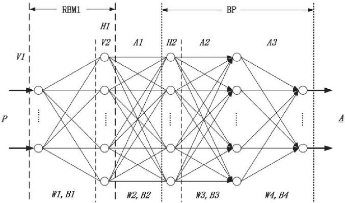
A deep belief network is composed of a deep Boltzmann machine and a classification part. Among them, the deep Restricted Boltzmann machine(RBM) is composed of three RBMs stacked in series. In addition, there is a BP network with a hidden layer, as shown in Figure 1.

Figure 1 Deep belief network structure.

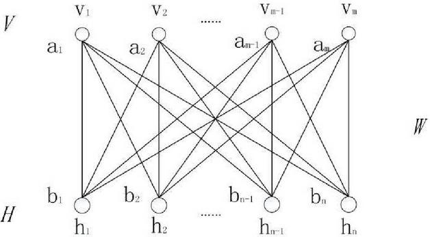
RBMs use unsupervised learning and are mainly used for feature extraction. BP network adopts supervised learning and is mainly used for classification or regression. Figure 2 shows the training process of a restricted Boltzmann machine. The RBM consists of a visible layer V and a hidden layer H, and its network structure is as follows.

Figure 2 Restricted Boltzmann machine training process.

The visible layer contains m nodes $V = (v_{1}, v_{2}, \dots v_{m - 1}, v_{m})$ , $v_{i} \in [0, 1]$ , and the hidden layer v contains n nodes $H = (h_{1}, h_{2}, \dots h_{n})$ $h_{i} \in [0, 1]$ . S sigmoid activation function is used between the visible layer and the hidden layer. $W = (w_{i j})$ represents the weight matrix between the visible layer and the hidden layer. $a = (a_{1}, a_{2}, \dots a_{m})$ represents the deviation from the visible layer V to the hidden layer H. $b = (b_{1}, b_{1}, \dots, b_{n})$ represents the deviation from the hidden layer H to the visible layer V.

DBN is a probabilistic generative model. Compared with traditional discriminative models of neural networks, generative models build a joint distribution between observations and labels. By training the weights between its neurons, the entire neural network can generate training data according to the maximum probability. Therefore, choosing this network is enough to learn more features.

4 Case Study

We chosen the GEFCom2012 competition dataset as the training set. By continuously adjusting the hidden layer of the DBN algorithm, the learning rate of the RBM, the learning rate of the fully connected layer, the number of iterations of the RBM, the number of iterations of the fully connected layer, the dropout ratio, and the activation function, the optimal short-term wind power prediction method is found. The purpose is to achieve optimal performance in different situations by adjusting different parameters of the deep belief network. The evaluation indicators used in this paper are mean square error (MSE) and R-squared, as shown in formula (1).

MSE = \frac{\sum_{i = 1}^{r} (n_{i} - 1) s_{i}^{2}}{N - r}

(1)

Where, N represents the number of data, r represents the number of groups, and the positive sample variance of the i-th group is si2.

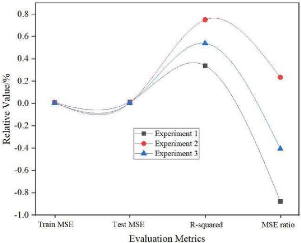
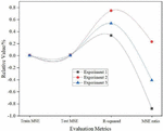
Figure 3 Predicted performance of Experiment 1, Experiment 2 and Experiment 3.

As can be seen from Figure 3, when these parameters in Experiment 1, Experiment 2, and Experiment 3 are set the same, including the hidden layer, the size of the RBM, the number of iterations of the RBM, the learning rate of the fully connected layer, and the learning rate of the RBM, and the number of iterations of the fully connected layer is set to 30, 12 and 28, respectively, the result of experiment 2 is the best. The training MSE, testing MSE and R-squared values in experiment 2 are 0.0094, 0.0072 and 0.2340, respectively. The R-squared value in experiment 2 is 0.641 and 0.1714 lower than the absolute value of experiment 1 and experiment 3, respectively. These three sets of experiments show that it is effective to adjust the number of iterations of the DBN fully connected layer without adjusting the dropout ratio, and the effect is more significant. The neural network parameter settings of these three groups of experiments are shown in Table 1.

Table 1 Parameter settings for Experiment 1, Experiment 2 and Experiment 3

Parameter Settings	Experiment 1	Experiment 2	Experiment 3
hidden layer	[250]	[250]	[250]
learning_rate_rbm	0.0005	0.0005	0.0005
batch_size_rbm	150	150	150
n_epochs_rbm	30	30	30
random_seed_rbm	500	500	500
learning_rate_nn	0.005	0.005	0.005
batch_size_nn	150	150	150
n_epochs_nn	30	12	28
dropout	/	/	0.5
activation_function_nn	tanh	tanh	tanh
train_mse	0.0088	0.0094	0.0037
test_mse	0.0165	0.0072	0.0052
r_squared	0.34	0.75	0.54
MSE ratio	$-$ 0.875	0.2340426	$-$ 0.405405405

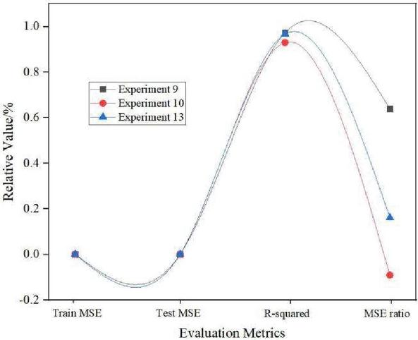
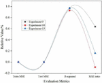
As can be seen from Figure 4, in Experiment 9, Experiment 10 and Experiment 13, the same parameters are set including the hidden layer, the learning rate of RBM, the size of RBM, the learning rate of RBM, the learning rate of the fully connected layer, and the fully connected layer. size, dropout ratio. The number of RBM iterations, the number of iterations of the fully connected layer, and the parameter settings of the activation function are different in Experiment 9, Experiment 10 and Experiment 13. When the activation function selection of experiment 9 and experiment 10 is the same, the number of iterations of the fully connected layer is gradually adjusted from large to small. It can be seen that the MSE ratio of experiment 10 is the lowest, which is 0.5483 lower than the absolute value of experiment 9. This shows that directly adjusting the number of iterations of the fully connected layer is also a way to improve the performance of the deep belief network algorithm when other parameters remain unchanged.

Figure 4 Predicted performance of Experiment 9, Experiment 10 and Experiment 13.

For Experiment 13, we adjusted the number of RBM iterations, the number of iterations of the fully connected layer, and the activation function. Although the experimental result is better than that of experiment 9, it is worse than that of experiment 10. This indicates that the choice of activation function should be non-linear as much as possible, and the linear learning performance is still relatively poor. The neural network parameter settings of these three groups of experiments are shown in Table 2.

Table 2 Parameter settings for Experiment 9, Experiment 10 and Experiment 13

Parameter Settings	Experiment 9	Experiment 10	Experiment 13
hidden layer	[100]	[100]	[100]
learning_rate_rbm	0.0005	0.0005	0.0005
batch_size_rbm	150	150	150
n_epochs_rbm	30	30	3
random_seed_rbm	500	500	500
learning_rate_nn	0.005	0.005	0.005
batch_size_nn	150	150	150
n_epochs_nn	30	20	29
dropout	0.5	0.5	0.5
activation_function_nn	relu	relu	linear
train_mse	0.0016	0.0011	0.000483
test_mse	0.00057724	0.0012	0.00040515
r_squared	0.973	0.93	0.967
MSE ratio	0.639225	$-$ 0.090909091	0.161180124

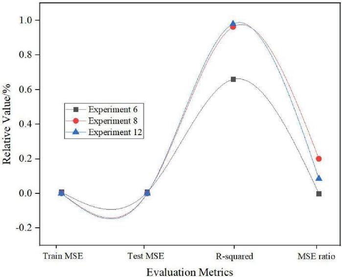
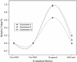
Figure 5 Predicted performance of Experiment 6, Experiment 8 and Experiment 12.

As can be seen from Figure 5, the same parameters set in Experiment 6, Experiment 8 and Experiment 12 include: hidden layer, learning rate of RBM, size of RBM, learning rate of RBM, learning rate of fully connected layer, and size of fully connected layer , dropout ratio. The number of RBM iterations, the number of iterations of the fully connected layer, and the parameter settings of the activation function are different in Experiment 6, Experiment 8 and Experiment 12. When the number of RBM iterations in Experiment 6 and Experiment 8 is the same, and different activation functions are selected, the experimental results will be very different. It can be seen that when the relu function is selected, the prediction effect is better than that of the sigmoid function. The R-squared value of Experiment 8 is 0303 higher than that of Experiment 6. This shows that when all parameter settings are the same, it is wiser for the activation function to prefer the relu function. In experiment 12, when the number of RBM iterations is reduced from 30 to 3, and linear is selected as the activation function, it is obvious that the R-squared value of this experiment increases linearly, which is 0.017 higher than that of experiment 8. From the above three experiments, it can be concluded that if the learning depth of the sample is not enough, the linear function is selected as much as possible, and the performance can be optimal. The neural network parameter settings of these three groups of experiments are shown in Table 3.

Table 3 Parameter settings for Experiment 6, Experiment 8 and Experiment 12

Parameter Settings	Experiment 6	Experiment 8	Experiment 12
hidden layer	[256]	[256]	[256]
learning_rate_rbm	0.0005	0.0005	0.0005
batch_size_rbm	150	150	150
n_epochs_rbm	30	30	3
random_seed_rbm	500	500	500
learning_rate_nn	0.005	0.005	0.005
batch_size_nn	150	150	150
n_epochs_nn	30	30	28
dropout	0.5	0.5	0.5
activation_function_nn	sigmoid	relu	linear
train_mse	0.0078	0.0011	0.00066372
test_mse	0.0078	0.00087922	0.00060666
r_squared	0.66	0.963	0.98
MSE ratio	0	0.200709091	0.085969987

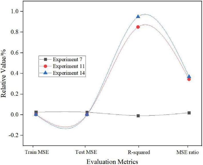
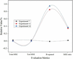
Figure 6 Predicted performance of Experiment 7, Experiment 11 and Experiment 14.

It can be seen from Figure 6 that the hidden layers of Experiment 7, Experiment 11, Experiment 14 and Experiment 15 are all selected to be double layers. These four groups of experiments set the same parameters including: RBM learning rate, RBM size, RBM iterations, RBM learning rate, learning rate of fully connected layer, size of fully connected layer, number of iterations of fully connected layer, dropout ratio. Experiment 7, Experiment 11 and Experiment 15 have the same number of nodes in the hidden layer, and other parameters are set the same, except for the selection of the activation function. It can be seen from these three sets of experiments that when the number of iterations is relatively small, a linear function is selected as the activation function, and the MSE value of experiment 15 is the smallest. This result is the same as mentioned earlier. Comparing Experiment 14 and Experiment 15, when the number of nodes in the hidden layer is increased, the effect of Experiment 14 is not very prominent. The conclusions drawn from the above four experiments are consistent with the previous experiments. The neural network parameter settings of these three groups of experiments are shown in Table 4.

Table 4 Parameter settings for Experiment 7, Experiment 11 and Experiment 14

Parameter Settings	Experiment 7	Experiment 11	Experiment 14
hidden layer	[100,100]	[100,100]	[256,256]
learning_rate_rbm	0.0005	0.0005	0.0005
batch_size_rbm	150	150	150
n_epochs_rbm	3	3	3
random_seed_rbm	500	500	500
learning_rate_nn	0.005	0.005	0.005
batch_size_nn	150	150	150
n_epochs_nn	30	30	30
dropout	0.5	0.5	0.5
activation_function_nn	sigmoid	relu	linear
train_mse	0.0249	0.0032	0.0019
test_mse	0.0244	0.0021	0.0012
r_squared	-0.0085	0.85	0.949
MSE ratio	0.020080321	0.34375	0.368421053

5 Conclusion

In conclusion, in order to find a method capable of forecasting wind power generation in a short period of time, we propose a short-term wind power generation forecasting method based on an optimized deep belief network approach. Based on GEFCom2012 competition dataset, the parameters of the deep belief network are continuously tuned through 15 sets of experiments. The results show that when the number of rbm iterations is small, the linear activation function is selected as much as possible; when the number of rbm iterations is large, the nonlinear activation function is selected as much as possible. The main reasons include two aspects: on the one hand, when the learning frequency is low, the linear function can learn the most obvious features more directly; On the other hand, when the learning frequency is high, the nonlinear function can learn the internal latent features more directly. The R-squared values of Experiment 4, Experiment 10 and Experiment 12 are the highest at 0.955, 0.93 and 0.98, respectively. The average R-squared value of these three tuned experiments is 0.2342 higher than the average of the other 12 experiments. In the future, we will continue to train and learn this model with data from different industries to make it more adaptable to more fields. Finally, the generalization ability of this model is improved.

Acknowledgements

This work was supported by the Science and Technology Projects of State Grid Gansu Electric Power Company (52272219100J).

References

[1] Liu D., Zhao D., Bai M., Wang Q. Analysis on Impact of Renewable Energy Generation on Real-time Electricity Price: Data Empirical Research on Electricity Spot Market of Germany. Automation of Electric Power Systems, 2020, (4): 27–29.

[2] Sun Y., Luo C., Ge Y. Economic Operation Optimization for New Energy Microgrid Based on Deterministic Method. Electric Power, 2020, 53(10): 149–155.

[3] Yang M., Jiang B. Recognition Method of Wind Curtailment Data Characteristics. Electric Power, 2017, 50(5): 95–100.

[4] Li S., Tu J., Shu Z. Dynamic Configuration Strategy for Frequency Regulation Reserve Capacity of Large-scale Wind Power for Promoting Peak Load Regulation. Automation of Electric Power Systems, 2020, 44(24): 53–59.

[5] Wu Z., Cheng S., Zhu C. Reconfiguration of Unbalanced Active Distribution Network Based on Linear Approximation Model. Automation of Electric Power Systems, 2018, 42(12): 134–141.

[6] Xu C., Li S. A method of wind diesel storage power distribution and operation prediction in a solitary island. Renewable Energy, 2020, (2): 54–55.

[7] Sheng S., Zhang L. Economic Dispatch of Power System Considering the Prediction Error of Wind Power,Solar Energy and Load. Automation of Electric Power Systems, 2017, 29(9): 80–85.

[8] Jiang C., Liu W., Yu L. Reliability Assessment of Power Generation System Considering Wind Power Penetration. Automation of Electric Power Systems, 2013, 25(4): 7–13.

[9] Ran X., Miao S., Liu Y. Modeling of Economic Dispatch of Power System Considering Joint Effect of Wind Power, Solar Energy and Load. Chinese Society for Electrical Engineering, 2014, (16): 2552–2560.

[10] Yang J., Wang X., Jiang C. Multi-objective dynamic optimal scheduling of power system considering wind power risk. Power System Protection and Control, 2016, 44(7): 25–31.

[11] Zhu B., Chen M., Xu R., Xu X. An optimal operation strategy of islanded microgrid. Power System Protection and Control. 2016, (15): 53–54.

[12] Chen X., Fu R. Research on the dual layer distributed scheduling algorithm for micro-grid connected mode. Microcomputers and Applications, 2016, 35(7): 79–82.

[13] Cheng B., Yang F., Wang Y. Interval optimization scheduling of electric vehicle charging station including wind power generation. Journal of Electrical Machinery and Control, 2021: 25(6): 101–109.

[14] Ma M., Shao L., Liu X. Application of distributed predictive control in coordinated control of microgrid. Journal of Jilin University (Engineering Edition), 2020, 50(6): 2258–2265.

[15] Zhao J., Guo S., Mu D. DouBiGRU-A: Software defect detection algorithm based on attention mechanism and double BiGRU. Computers & Security, 2021, (111): 102459.

[16] Zhao J., Zhang X., Di F. Exploring the Optimum Proactive Defense Strategy for the Power Systems from an Attack Perspective. Security and Communication Networks, 2021, 2021.

[17] Yu Z., Lu X., Sun L., Xiong J., Ye L., Li X., Zhang R., Ji N. Metal-Loaded Hollow Carbon Nanostructures as Nanoreactors: Microenvironment Effects and Prospects for Biomass Hydrogenation Applications. ACS Sustainable Chemistry and Engineering, 2021, 9(8): 2990–3010.

[18] D Panasetsky, D Tomin, N Karamov, D Zhukov, A Muftahov, I Dreglea, A Liu, F Li, Denis Panasetsky, Daniil Tomin, Nikita Karamov, Dmitriy Zhukov, Fang Li. Toward Zero-Emission Hybrid AC/DC Power Systems with Renewable Energy Sources and Storages: A Case Study from Lake Baikal Region. Energies, 2020, 13(5): 1226.

[19] Fan C., Ding C., Zheng J., Xiao L., Ai Z. Empirical Mode Decomposition based Multi-objective Deep Belief Network for short-term power load forecasting. Neurocomputing, 2020, 388(0): 110–123.

Biographies

Yiming Zhang, graduated from Northeast Electric Power University in 2012 with a bachelor’s degree in transmission engineering and a bachelor’s degree in power system automation. In 2020, he obtained a master’s degree in electrical engineering from North China Electric Power University. Zhang Yiming has been working in State Grid Gansu Electric Power Company since 2012. As an electrical engineer and professional, he has extensive experience in the operation and maintenance of transmission lines and drone inspection management. He was responsible for the autonomous inspection business of drones and the construction of digital management and control platform, and the cultivation and optimization of artificial intelligence image recognition technology of the State Grid Gansu Electric Power Company. In addition, he also presided over the large-scale application of drones in the inspection and maintenance of overhead transmission lines of Gansu Electric Power Company.

Cheng Li, she graduated from Lanzhou Jiaotong University in 2014 with a bachelor’s degree in electrical engineering and automation. Cheng Li has been working at State Grid Gansu Electric Power Company since 2014. He was responsible for the low-carbon energy service station project, researched on energy storage, photovoltaics, and optical fiber lighting, and was awarded by the State Grid Corporation. As an electrical engineer and professional, rich experience in power grid planning, line loss management, power marketing management.

Distributed Generation & Alternative Energy Journal, Vol. 37_6, 1739–1754.
doi: 10.13052/dgaej2156-3306.3761
© 2022 River Publishers