Nodal Electricity Price Forecasting using Exponential Smoothing and Holt’s Exponential Smoothing

Md Irfan Ahmed^* and Ramesh Kumar

National Institute of Technology Patna, Department of Electrical Engineering, Bihar, India
E-mail: irfannitp.ahmed@gmail.com; ramesh@nitp.ac.in
*Corresponding Author

Received 29 September 2022; Accepted 19 December 2022; Publication 10 July 2023

Abstract

The prediction of nodal electricity price (NEP) is a primary step to be done before the bidding process starts in the actual market environment. NEP plays a significant role for the efficient working of the electrical system. NEP follows a common trend as during peak hours when the load is high the price will also be high similarly during off-peak-load times the price will be lower and common to all the node. Thus, accurate forecasting of the NEP can help electricity generation companies to be more proactive in the wholesale electricity market to maximize its overall benefits. In this paper, exponential smoothing (ES), and holt’s exponential smoothing (HES) have been utilized for forecasting the NEP. Furthermore, a comparative analysis between ES and HES has been done considering several alpha values and several trends. The model evaluation and the forecasting performance have been tested using different parameters of ES, and HES techniques such as Akaike Information Criterion (AIC), Akaike Information Criterion Corrected (AICc), Bayesian Information Criteria (BIC). The performance of the proposed technique has been authenticated efficaciously on average nodal real-time price data collected from ISO New England (BOSTON Zone).

Keywords: Nodal electricity price (NEP), electricity load forecasting (ELF), exponential smoothing (ES), Holt’s exponential smoothing (HES).

1 Introduction

Nodal electricity price (NEP) plays a crucial role in the development of the nodal electricity market (EM). For maximizing profitability, NEP is very essential for all the electricity market participants such as generating companies, sellers, buyers, and investors [1, 2]. EM always maintains the balance between generation and consumption because it can’t be stored at a large level for economic reasons [3]. Market-Clearing Price (MCP) is a basic pricing tool. It can be used to show the numerous zones and buses in electrical networks where there is no transmission congestion. Whenever locational marginal price (LMP) would be employed in the congested line, electricity prices (EPs) will be increased in congested areas. LMPs would be predicted for each bus in the entire power system. LMP is the cost of delivering the next MW of load at a particular location (node), taking into account the generation marginal cost, transmission congestion cost, and losses [4]. LMP is the same as MCP with no congestion. LMP is also known as nodal pricing. Load forecasting is a significant feature in the improvement of any model for power planning, especially in the present-day transforming power system structure [5]. The LMP method is the primarily used pricing technique in the EM such as New York, California, New England Independent System Operator [6]. Electricity load forecasting (ELF) represents a very important role in the preparation of consumers’ necessities, operations, and maintenance in the EM. Electrical load depends on the consumption of electrical energy. In our day-to-day life, electrical power is a vital issue for growth of the country. The EP and consumption depend on the non-renewable energy that is increasing rapidly. The development of ELF to satisfy the growing needs of power is a great challenge for the country. To store electrical power in a buffer is a challenging task hence, to confirm the appropriate distribution of electrical power to customers, it is essential to forecast electricity load (EL).

There has been a large number of economic and statistical models for the EP and load forecasting (LF) put up in the literature over the years. L. Hu, G. Taylor, and M. Irving et al. [2] presented that the power distributor uses a fuzzy logic technique for the optimal bidding schemes for achieving maximum profits in the competitive UK EM. In [1], presented optimal bidding techniques for the energy distributor in UK EM. R. Weron et al. [3] represented the electricity price forecasting (EPF) review, error evaluation, and also, it’s statistical testing. V. Bianco, O. Manca, and S. Nardini et al. [7] proposed long-term electricity consumption forecasting in Italy. In the first stage evaluation of price and electricity consumption is done. While in the second stage different regression models and their statistical tests are done in the proposed models. Power consumption and economic development in Turkey were described by U. S. Ramazan Sari et al. [8] using several sources of power consumption and employment. J.-C. JuliánPérez-Garcíaa et al. [9] presented an analysis of electricity demand using a simple growth rate decomposition technique. This technique develops a long-term prediction model to obtain the predictions of energy demand in Spain till 2030. H. Daneshi et al. [4] gave a brief survey of different methodologies and their development in the field of EP forecasting. H. Zheng et al. [10] represented forecasting the electricity price using GARCH. EP is considered an economic time series and analyzes its volatility, which illustrates the existence of heteroskedasticity. Next, a price prediction is developed using the GARCH model, which aims to estimate the price. The case studies evidence supports the validity of the suggested model. R. Y. Ksenia Letovaa et al. [11] discussed on Russian electricity market background and its targets. B. Han et al. [12] proposed an ideal grid-connected microgrid using demand profile forecasts. Y. Yu et al. [13] proposed enhanced Dragonfly algorithm-based support vector machine for forecasting offshore wind power. Y. Liang et al. [14] suggested the enhanced deep belief network to forecast the renewable energy loads. S. Borovkova and M. D. Schmeck et al. [15] proposed EP modeling, dependent on the stochastic time change. The stochastic time change presents stochastic along with deterministic characteristics in the price method volatility and the jump component. X. Xu et al. [16] proposed the full-cost electricity pricing to provide an integrated approach for power supply, power grid, and load. F. Xianyu et al. [17] proposed the secure power system optimal dispatch model that includes electricity pricing demand response. G. Lei et al. [18] described the hybrid approach for predicting the electricity price of the Iranian EM that utilizes both multi-layer perceptron and radial basis function.

Most of the available research has not provided an insight into the electricity forecasting techniques that could be used for the nodal electricity market. As a result, a research gap has been found in this circumstance, and our manuscript is the most suited one to fill that gap. The novel approach presented in this manuscript intends to forecast the NEP using ES, and HES techniques with the help of several values of alpha, and different trends. In this way our approach performs better for the NEP forecasting. In this paper, the nodal electricity market model is the most advantageous solution is to be used that optimizes the price in the EM. So, here in this work efforts are on NEP forecasting. Last but not least the summary of various electricity market price and load forecasting models is presented in Table 1.

Table 1 Summary of various electricity markets price and load forecasting

			Attributes
References	Electricity Market	Model Type	Load/Demand	Price
[4]	New England	GARCH		$\mathrm{✓}$
[7]	Italian Electricity Market	Linear Regression (LR), Support Vector Regression (SVR)	$\mathrm{✓}$
[19]	Italian Electricity Market	Neural Network		$\mathrm{✓}$
[20]	Day-ahead, Rajasthan state electricity board	ANFIS	$\mathrm{✓}$
[21]	Greek and Hungarian Day ahead EM	Support Vector Machine		$\mathrm{✓}$
[22]	PJM Power Market	Convolutional Neural Network		$\mathrm{✓}$
[23]	PJM Power Market	LSSVM (Least Squares Support Vector Machine), ARMAX (Autoregressive Moving Average with External Input)		$\mathrm{✓}$
[24]	New South Wales (NSW Australia Market)	Empirical Mode Decomposition, SVR, PSO, AR-GARCH Model	$\mathrm{✓}$
[25]	Indian Electricity Market	Autoregressive GARCH Model		$\mathrm{✓}$
[26]	Australian National Electricity Market	Principle Component Analysis (PCA), Granger Casuality network		$\mathrm{✓}$
[27]	German/Austrian Power Market	ANN		$\mathrm{✓}$
[28]	PJM and Australia Electricity Market	Dynamic Choice ANN		$\mathrm{✓}$
[29]	Mainland Spain	PCA/Nonparametric models	$\mathrm{✓}$	$\mathrm{✓}$
[30]	ISO New England	Autoregression, NARX neural network		$\mathrm{✓}$
[31]	Australia Electricity Market	Multilayer neural network		$\mathrm{✓}$
[32]	New York Independent System Operator	Quadratic Programming		$\mathrm{✓}$
[33]	Western Danish	ARMA, Holt-winters	$\mathrm{✓}$	$\mathrm{✓}$
[34]	Mainland Spain and California Markets	ARIMA		$\mathrm{✓}$

1.1 Motivation

To the author’s knowledge and reviewing the previous literature regarding ES, and Holt’s ES techniques it has been concluded that these techniques have not been properly implemented so far for NEP in the electricity market. The NEP are highly volatile, posing a rise to substantial price and load risk for the nodal EM. As a result, it has inspired us to give more emphasis to the NEP forecasting.

1.2 Contributions

The main contribution of the paper has been listed below: –

• The modeling of nodal EM as an additional advantage has been developed.

• The authors have represented the various forecasting techniques and influence factors for the NEP.

• The ES method has been applied to a number of different alpha values, and the results show that optimal alpha provides the best predicting accuracy with the lowest possible values of AIC, AICc, and BIC for NEP.

• Additionally, the HES methodology has been applied to a number of trends, and the outcomes have shown that additive damped trends provide the most accurate forecasts, with the lowest values of AIC, AICc, and BIC for NEP.

1.3 Organization of the Paper

The hierarchy of the paper have been prepared as follows: Section 2 presents the various influencing factor of NEP and benefits of the nodal electricity market whereas, Section 3 describes the classification of EPF. Section 4 discusses the problem formulation and its proposed methodology such as ES, and HES. Section 5 summarizes the results while Section 6 concludes the paper.

2 Nodal Electricity Price Influence Factors

An EM depends on the price and load because the buyer wants to buy the electricity at a lower price and the seller wants to sell at a higher price. The price will be decided by the electricity consumption. Hence, there are many factors, which influence the different types of the electricity market. The electricity price influenced by these six factors are categorized as namely, weather conditions, seasons, fuel cost, supply, demand, and government regulations. There are also numerous factors which cause the fluctuation an NEP.

Examples of NEP influence factors: - Gross Domestic Product (GDP) [7], People income level [8], Employment rate [9], etc. The major effects of NEP are shown in Figure 1.

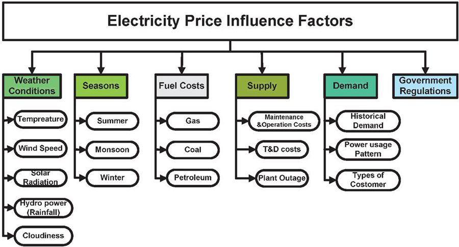
Figure 1 Nodal electricity price influence factor.

2.1 Benefits of Nodal Electricity Market [35]

The paper utilizes the data of nodal electricity market of New England, Boston Region for validation purpose. The benefits of having a nodal electricity market have been listed below:

• The nodal electricity market includes the production cost as well as energy transmission cost.

• Better usage of the system by decreasing security margins.

• Transparency and reasonable prices for EM customers.

• The model is beneficial to business novelty.

3 Classification of EP Forecasting

Forecasting is a methodology that uses historical data (present and past data) as inputs to estimate the prediction of future trends. Forecasts are used by the EM to determine how to distribute their expenses or to plan for projected costs in the future. The various approaches have been developed for EPF where most of the algorithms are employed in LF and particularly short-term LF, and other applications. The comparison of EP prediction algorithms is shown in Table 2.

Table 2 Comparison of seven types of optimization algorithms for electricity price prediction

References	Methods	Merits	Demerits
[24]	PSO	• To maximize the power Quality • Less computing space (memory) • High convergence compared to GA	• Difficult to design initial parameters • Premature convergence and trapped to local minima
[19, 27, 28]	ANN	• Easy model building with less formal statistical information required • Capable of capturing non-linearity’s between predicators and outcomes	• Takes longer time to process of large neural network • Black box nature
[25]	GARCH Model	• To estimate maximum-likelihood function • It has probabilistic information about the future market range	• It can’t be estimated using the least square function
[34]	ARIMA	• Appropriate for non-stationary time series • Stability • High accuracy prediction	• Unable to respond immediately
[26, 29]	PCA	• It has low sensitivity noise • Decreased requirements for capacity and memory	• Independent variable becomes less interpretable • Data standardization is must before PCA
[21]	Support Vector Machine	• High accuracy • Consist of non-linear transformation	• Increased Speed and size requirements for machine learning algorithms
[31]	Multilayer Neural Network	• It is used for deep learning	• It includes too many parameters • Complex design and maintain

3.1 Electricity Price Forecasting Methods

The EPF is categorized into three groups that are Data mining, Time series, and Simulation model technique. The EPF model is shown in Figure 2.

3.2 Time Series Model

Time series forecasting is a significant area of artificial intelligence because numerous forecasting issues including a time component is resolved by a time series model. Mostly specified time-series models are:

(1) Linear Regression

Regression is a form of predictive modeling approach which inspects the connection between two variables, one which is dependent and the other is an independent variable. The following are three main applications in regression analysis: –

(a) Identifying the strength of predictors: – It’s used to evaluate the strength of the influence independent variables have on a dependent variable.

(b) Influence of Forecasting: – It’s used to predict the effect of changes. To comprehend the regression analysis how much the dependent variable variations with a variation in one or more independent variables.

(c) Trend forecasting: – It is used to predict trends and future values.

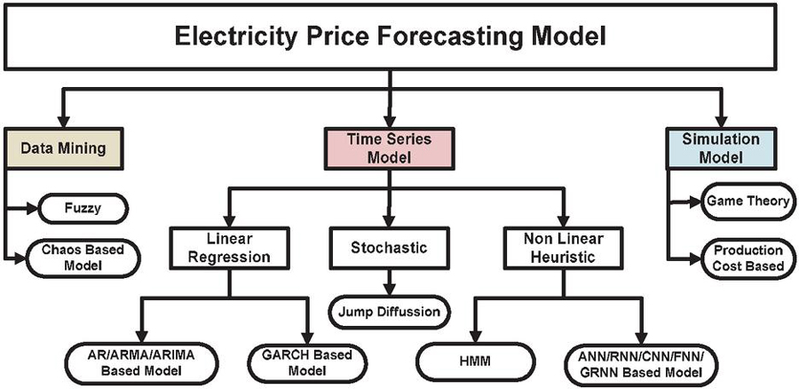
Figure 2 Electricity price forecasting model.

LR is statistics and a machine learning algorithm. The LR model attempts to find the connection amongst the two variables (input variables (x) and the single output variable (y)) by fitting the linear equation to observed data.

We are familiar with the equation that is y $=$ mx $+$ c.

Where y is the dependent variable; m is the slope or gradient, and c is the intercept. LR a single independent variable and is used to forecast the value of a dependent variable is represented in Equation (1):

$$\mathrm{y}={\delta }_0+{\delta }_1{\mathrm{x}}_1+\mathrm{\cdots }+{\delta }_{\mathrm{r}}{\mathrm{x}}_{\mathrm{r}}+\text{e}$$

(1)

Where, ${\delta }_0,{\delta }_1,\mathrm{\dots },{\delta }_{\mathrm{r}}$ are the regression coefficients, and eis the random error. In Figure 3 displays the linear regression model in which x-axis represents the hours and y-axis represent the price.

Regression Forecasting Performance

Regression coefficient of determination (R${}^2$) indicates how much amount of variation in y can be explained by the reliance on x by the given regression model.

• A higher R${}^2$ indicates a better fit, and the model can better describe the variation of the output with different inputs.

• The value of R${}^2=0.7$ to 1 corresponds to the sum of squared residuals $=$ 0, is the most accurate fit, since the values of forecasted and actual responses fit entirely to each other.

${\mathrm{R}}^2$	$=1-{\displaystyle \frac{\mathrm{Sum}\mathrm{of}\mathrm{Residuals}({\mathrm{SS}}_{\mathrm{res}})}{\mathrm{Sum}\mathrm{of}\mathrm{Mean}({\mathrm{SS}}_{\mathrm{mean}})}}$	(2)
${\mathrm{SS}}_{\mathrm{res}}$	$={\displaystyle \frac{1}{\mathrm{n}}}{\displaystyle \sum _{\mathrm{i}=1}^{\mathrm{n}}}{(\mathrm{y}-\mathrm{y}\mathrm{\_}\mathrm{predicted})}^2$	(3)
${\mathrm{SS}}_{\mathrm{mean}}$	$={\displaystyle \frac{1}{\mathrm{n}}}{\displaystyle \sum _{\mathrm{i}=1}^{\mathrm{n}}}{(\mathrm{y}-\overline{\mathrm{y}})}^2$	(4)
${\mathrm{SS}}_{\mathrm{mean}}$	$>{\mathrm{SS}}_{\mathrm{res}}$	(5)

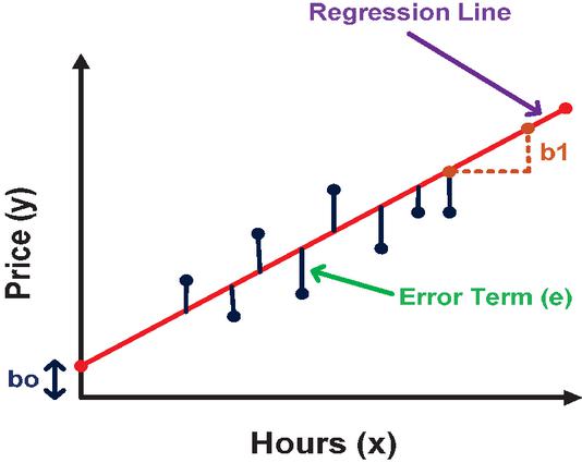
Figure 3 Linear regression model.

(2) GARCH Model

The GARCH model is an acronym that stands for generalized autoregressive conditional heteroskedasticity. The objective of the GARCH model is to provide variance measurements for heteroscedastic time series data, ad similarly standard deviations are viewed in the simplified models. In economics and finance, GARCH models can be used to evaluate the time series data in several ways. It is particularly beneficial when there are phases of fast-changing variation (or volatility).

The GARCH (p,q) method is given in the following sections [10]: –

${\sigma }_{\mathrm{t}}=\omega +{\displaystyle \sum _{\mathrm{j}=1}^{\mathrm{p}}}{\beta }_{\mathrm{j}}{\sigma }_{\mathrm{t}-\mathrm{j}}+{\displaystyle \sum _{\mathrm{i}=1}^{\mathrm{q}}}{\alpha }_{\mathrm{i}}{\mathrm{e}}_{\mathrm{t}-\mathrm{i}}^2$	(6)
$\omega >0,{\alpha }_{\mathrm{i}}\ge 0,{\beta }_{\mathrm{j}}\ge 0$
${\displaystyle \sum _{\mathrm{i}=1}^{\mathrm{q}}}{\alpha }_{\mathrm{i}}{\mathrm{e}}_{\mathrm{t}-\mathrm{i}}^2\Rightarrow \mathrm{ARCH}\mathrm{Term}$
${\displaystyle \sum _{\mathrm{j}=1}^{\mathrm{p}}}{\beta }_{\mathrm{j}}{\sigma }_{\mathrm{t}-\mathrm{j}}\Rightarrow \mathrm{GARCH}\mathrm{Term}$

wherever, the (p,q) in comments is a common representation in which the p specifies the number of autoregressive lags included in the equation and q specifies the number of lags is involved in the Moving Average (MA) component of a variable.

From Equation (6), the conditional variance is a linear function of q lags the squares of the error terms (e${}_{\mathrm{t}}^2$) or ARCH (autoregressive conditional heteroskedasticity) terms and p lags of the historical values of the conditional variances (${\sigma }_t$) or the GARCH terms, and a constant $\omega$.

A GARCH model follows 3 fundamental steps:

1. Calculate the most suitable autoregressive model.

2. Determine the autocorrelations of the error term

3. Test with statistical significance.

(3) ARIMA Model

A modification of basic Auto-Regressive Moving Average incorporates with the integration that is ARIMA. This abbreviation conveys the most important aspects of the model. The following are the brief description of them:

• AR (Autoregression): – A model based on the relationship between an observation and a number of lagged observations.

• I (Integrated): – To maintain the time series stationary, the difference between raw data (e.g., subtracting an observation from the previous time step) is used.

• MA: – A model that highlights the connection between an observation and a residual error from a MA model applied to lagged data.

Parameters are used to represent each of these elements in the model. This is typical notation for ARIMA (p,d,q) in which the parameters are replaced by integer values to make it easier to identify the ARIMA model being used. The ARIMA model includes the following variables:

p: The lag order refers to the number of lag observations in the model.

d: The degree of difference is the no. of times that the raw observations are differenced.

q: The MA window size, which is referred to as the MA order.

(4) Stochastic Model

Jump diffusion is a stochastic process that includes jump and diffusion. It has applications in Price forecasting and pattern theory in physics. The jump-diffusion model was developed to try to describe non-continuous (i.e., gapping) price behavior in the electricity market. The formula is the geometric Brownian motion and jumps are assumed to be the sources of unpredictability in the EM and prices. It is written as in Equation (7) as:

${\displaystyle \frac{{\mathrm{dS}}_{\mathrm{t}}}{{\mathrm{S}}_{\mathrm{t}}}}=\mu \mathrm{dt}+\sigma {\mathrm{dW}}_{\mathrm{t}}+(\mathrm{J}-1)\mathrm{dN}(\mathrm{t})$	(7)
${\displaystyle \frac{{\mathrm{dS}}_{\mathrm{t}}}{{\mathrm{S}}_{\mathrm{t}}}}\mathrm{change}\mathrm{in}\mathrm{EP}$

Where $\mu$dt is the drift due to the risk-free rate, $\sigma$dW${}_{\mathrm{t}}$ is the Geometric Brownian motion for specified volatility, and (J–1)dN(t) factors the size of the jump as a percentage of the EP and the probability of a certain number of jumps will occur. EP jumps are often considered to follow a probability rule. For example, Poisson processes, are continuous-time discrete processes that may be used in the model. In the interval [0, t], at a particular time t, let us assume X${}_{\mathrm{t}}$ is the number of times a special event. Then X${}_{\mathrm{t}}$ represents a Poisson process if

$${\mathrm{P}}_{\mathrm{r}}({\mathrm{X}}_{\mathrm{t}}=\mathrm{m})=\frac{{\lambda }^{\mathrm{m}}{\mathrm{t}}^{\mathrm{m}}}{\mathrm{m}!}\exp (-\lambda \mathrm{t})$$

(8)

X${}_{\mathrm{t}}$ depicts the Poisson distribution with parameter ${\lambda }_{\mathrm{t}}$. The parameter $\lambda$ governs the occurrence of the special event and is mentioned as the rate.

(5) Hidden Markov Model

It is a specific type of mathematical model in which the system is modeled through Markov method that is termed as hidden states. The Hidden Markov model is the process in which the behavior of Y depends on X. The main aim is to learn X by observing Y.

(6) Moving Average (MA)

The primary benefit of MA is that it provides a smoothed line which is less prone to whipsawing up and down concerning minor, transitory price fluctuations. MA forecasts the future points by using an average of several past data points. It is a classical method of time series forecasting. MA of order m, T${}_{\mathrm{t}}$ is calculated as:

$${\mathrm{T}}_{\mathrm{t}}=\frac{1}{\mathrm{m}}\sum _{\mathrm{j}=-\mathrm{k}}^{\mathrm{k}}{\mathrm{y}}_{\mathrm{t}+\mathrm{j}}$$

(9)

Where, m $=$ 2k+1; to evaluate the trend-cycle at time t is achieved by averaging values of the time series within k periods of t.

4 Problem Formulation and Methodology

The NEP problems is formulated based on the two scenarios such as ES, and Holt’s ES. The benefits of ES are that it reacts to EP fluctuations more rapidly. Due to the fact that the ES shows trend shift more quickly, this is especially beneficial to bidders looking to bid the electricity in the competitive EM. ES is used for time series forecasting where the dataset doesn’t follow any trend or seasonality.

(a) Trend: – Upward and downward slope

(b) Seasonality: – It shows the specific pattern due to seasonal factors like hours, days, years, etc.

ES works on a weighted average i.e., the average of the previous period and current observation. The most recent observations have the highest weights, while the earliest observations have the lowest weights. Weights are controlled by smoothing parameters. ES is calculated by: –

${\mathrm{Y}}_{\mathrm{t}+1}$	$={\mathrm{Y}}_{\mathrm{t}}+\alpha ({\mathrm{A}}_{\mathrm{t}}-{\mathrm{Y}}_{\mathrm{t}})$	(10)
${\mathrm{Y}}_{\mathrm{t}+1}$	$=\alpha {\mathrm{A}}_{\mathrm{t}}+(1-\alpha ){\mathrm{Y}}_{\mathrm{t}}$	(11)

Smoothing Constant: $0\le \alpha \le 1$

Where; A${}_{\mathrm{t}}$ is actual nodal EP for the period, Y${}_{\mathrm{t}}$ is forecast for the previous period. The weighting is defined by the smoothing parameter $\alpha$, which should be larger than 0 and less than 1. If $\alpha =0$, the smoothed point will be reset to its prior value, and if $\alpha =1$, the smoothed point will be reset to the current point.

Various other exponential smoothing models work on time series forecasts namely: –

(1) Holt’s method: – It is used when the datasets follow a specific trend like upward or downward [36] as given below: –

(a) Holt’s linear trend method: –

This technique consists of a prediction and two smoothing equations, one for level and the other for trend [36].

$\mathrm{Forecast}\mathrm{equation}{\widehat{\mathrm{y}}}_{\mathrm{t}+\mathrm{h}|\mathrm{t}}={\mathrm{l}}_{\mathrm{t}}+{\mathrm{hb}}_{\mathrm{t}}$	(12)
$\mathrm{Level}\mathrm{equation}{\mathrm{l}}_{\mathrm{t}}=\alpha {\mathrm{y}}_{\mathrm{t}}+(1-\alpha )({\mathrm{l}}_{\mathrm{t}-1}+{\mathrm{b}}_{\mathrm{t}-1})$	(13)
$\mathrm{Trend}\mathrm{equation}{\mathrm{b}}_{\mathrm{t}}={\beta }^{*}({\mathrm{l}}_{\mathrm{t}}-{\mathrm{l}}_{\mathrm{t}-1})+(1-{\beta }^{*}){\mathrm{b}}_{\mathrm{t}-1}$	(14)

Where l${}_{\mathrm{t}}$ and b${}_{\mathrm{t}}$ evaluate the level and trend of the series at time t. $\alpha$ is the level smoothing constant for $0\le \alpha \le 1$ and ${\beta }^{*}$ is the trend smoothing constant for $0\le {\beta }^{*}\le 1$.

(b) Holt’s additive damped trend method: –

This technique consists of damping parameters $\phi$ ($0<\phi <1$).

$\mathrm{Forecast}\mathrm{equation}{\widehat{\mathrm{y}}}_{\mathrm{t}+\mathrm{h}|\mathrm{t}}={\mathrm{l}}_{\mathrm{t}}+(\phi +{\phi }^2+\mathrm{\cdots }+{\varphi }^{\mathrm{h}}){\mathrm{b}}_{\mathrm{t}}$	(15)
$\mathrm{Level}\mathrm{equation}{\mathrm{l}}_{\mathrm{t}}=\alpha {\mathrm{y}}_{\mathrm{t}}+(1-\alpha )({\mathrm{l}}_{\mathrm{t}-1}+\phi {\mathrm{b}}_{\mathrm{t}-1})$	(16)
$\mathrm{Trend}\mathrm{equation}{\mathrm{b}}_{\mathrm{t}}={\beta }^{*}({\mathrm{l}}_{\mathrm{t}}-{\mathrm{l}}_{\mathrm{t}-1})+(1-{\beta }^{*})\phi {\mathrm{b}}_{\mathrm{t}-1}$	(17)

If $\phi =1$ then this technique is similar to Holt’s linear method. The range of $\phi$ is [0,1] dampens the trend so that it approaches a constant time in the future.

(c) Holt’s exponential smoothing method: –

Holt’s ES has two smoothing constants that represent the weight to evaluate the trend of the data and range of 0 to 1.

$\mathrm{Forecast}\mathrm{equation}:{\widehat{\mathrm{y}}}_{\mathrm{t}+\mathrm{m}}={\mathrm{l}}_{\mathrm{t}}+{\mathrm{b}}_{\mathrm{t}}(\mathrm{m})$	(18)
$\mathrm{Level}\mathrm{equation}:{\mathrm{l}}_{\mathrm{t}}=\alpha {\mathrm{X}}_{\mathrm{t}}+(1-\alpha )({\mathrm{l}}_{\mathrm{t}-1}+{\mathrm{b}}_{\mathrm{t}-1})$	(19)
$\mathrm{Trend}\mathrm{equation}:{\mathrm{b}}_{\mathrm{t}}=\gamma ({\mathrm{l}}_{\mathrm{t}}-{\mathrm{l}}_{\mathrm{t}-1})+(1-\gamma ){\mathrm{b}}_{\mathrm{t}-1}$	(20)

4.1 Scenario 1: – Algorithm for Price Forecasting using Exponential Smoothing

Step 1 – Import the stats model library

Step 2 – Load the nodal electricity price datasets from the year 2004 to 2020.

Step 3 – Visualize and analyze the nodal electricity price datasets and create a time series of the dataset. The frequency of the time series is monthly so, pass the argument “M” in the series function.

Step 4 – Analyze the data using the line chart and use the plot library for visualization.

Step 5 – Forecast the model using exponential smoothing, take smoothing level $\alpha$ (alpha) value. Now, create the three instances for three different values of $\alpha$ i.e., $\alpha =0.2$, $\alpha =0.6$, optimum $\alpha =0.9999999850988388$, $\alpha$ value is automatically optimized by stats model.

Step 6 – Now, pass the datasets into exponential smoothing and fit the datasets with different values of smoothing level. The minimum AIC gives the best prediction model.

4.2 Scenario 2: – Algorithm for Price Forecasting using Holt’s Exponential Smoothing

Step 1 – Import the stats model library

Step 2 – Load the nodal electricity price datasets from the year 2004 to 2020.

Step 3 – Visualize and analyze the nodal electricity price datasets and create a time series of the dataset. The frequency of the time series is monthly so, pass the argument “M” in the series function.

Step 4 – Forecast the model using Holt’s exponential smoothing, take smoothing level $\alpha$ (alpha) value. Now, create the three instances for three different trends. The three different trends are linear, exponential, additive damped trends for $\alpha =0.8$, smoothing slope $=$ 0.2, is optimized by the stats model.

Step 5 – Now, pass the datasets into Holt’s exponential smoothing and fit the datasets with the three different trends. The minimum AIC gives the best model for prediction.

5 Simulation and Results

Monthly average real-time electricity price data for Boston regions of ISO New England Electricity market from 2004 to 2020 is used for the research to estimate the NEP forecasting performance of the calibrated models [37]. Figure 4 represents the nodal electricity price, line plot from the year 2004 to 2020.

5.1 Scenario 1: Forecasting using ES

ES technique is used for EPF. The associated equations are accessible from Equation (10). In this paper, forecasting consists of three different smoothing levels that are at $\alpha =0.2$, $\alpha =0.6$, and at optimum alpha as shown in Figures 5–8. The comparison of the forecasted price using ES at three different smoothing levels is shown in Figure 8. The algorithm used for model selection is based on AIC. Model selection is a process in which to compare the relative AIC value of various models and find the best fit model for the observed data. Model evaluation and selection are done from Table 3. The forecasted outcome shows that the optimum alpha is a better prediction than the other two levels because the value of AIC, AICc, and BIC is minimum at Model-3 as shown in Table 3.

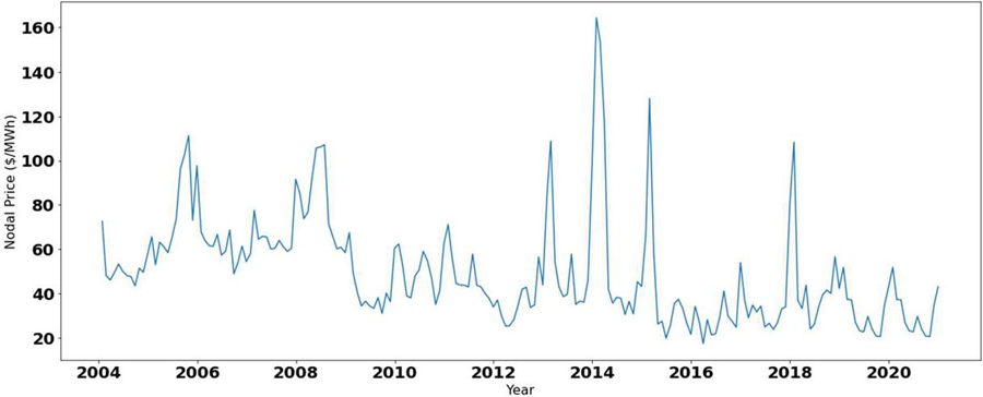
Figure 4 Nodal electricity price line plot from the year 2004 to 2020.

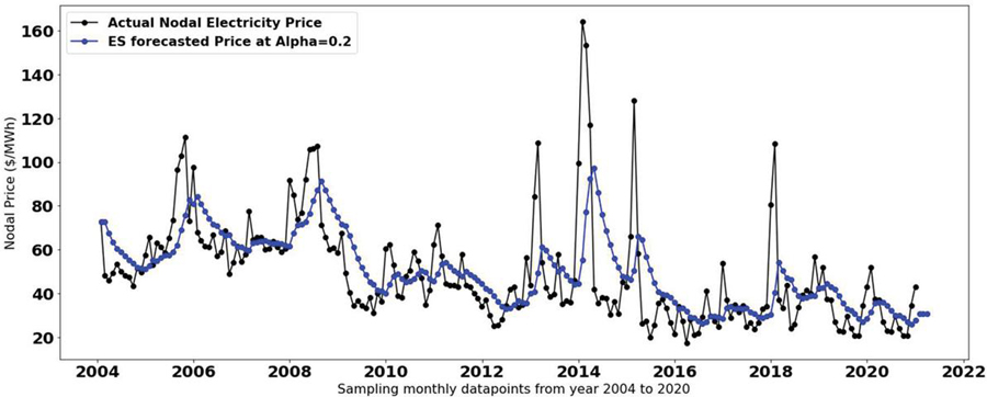
Figure 5 Forecasted plot of nodal electricity price using ES at alpha $=$ 0.2.

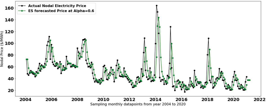
Figure 6 Forecasted plot of nodal electricity price using ES at alpha $=$ 0.6.

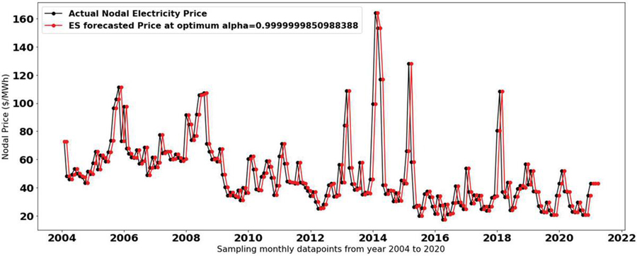
Figure 7 Forecasted plot of nodal electricity price using ES at optimum alpha.

Figure 8 Comparison plot of nodal electricity price using ES for a different mode.

5.2 Scenario 2: Forecasting using Holt’s ES

Holt’s ES method is used for price forecasting. The related equations are presented in (12)–(20). In this technique, forecasting consists of three trends that are linear, exponential, and additive damped trends as shown in Figures 9–12. The comparison of the results of forecasting by the above-mentioned three trends is presented in Figure 12. The prediction results show that in this paper the additive damped trend method yielded a better prediction than linear and exponential because the value of AIC is minimum in model-3 as shown in Table 4.

Table 3 Model evaluation and selection of ES

Parameters	Model-1	Model-2	Model-3
AIC	1227.436303	1178.314583	1155.624743
AICc	1227.637308	1178.515588	1155.825748
BIC	1234.072543	1184.950823	1162.260983

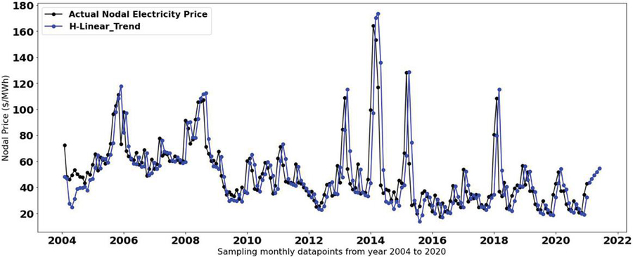
Figure 9 Forecasted plot of nodal electricity price using Holt’s ES for linear trend.

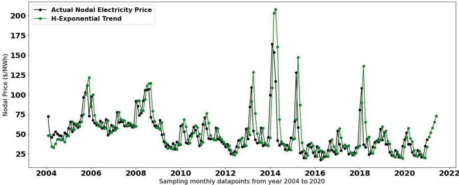
Figure 10 Forecasted plot of nodal electricity price using Holt’s ES for exponential trend.

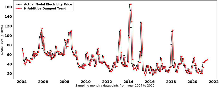
Figure 11 Forecasted plot of nodal electricity price using Holt’s ES for additive damped trend.

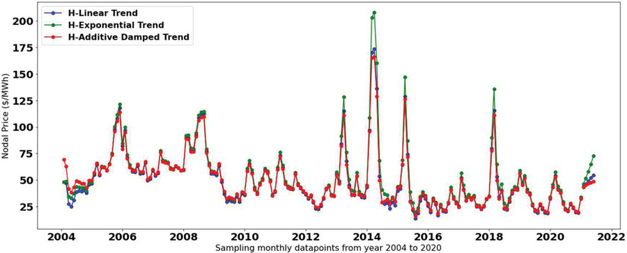
Figure 12 Comparison plot of nodal electricity price using Holt’s ES for different trends.

5.3 Model Evaluation and Selection

The three important metrics for model evolution and selection in ES and Holt’s ES are shown in Tables 3 and 4. AIC was developed by Hirotugu Akaike et al., in 1970. AIC is a statistical test that determines how well the model fits the data. To prevent, over-fitting it penalizes the models with more independent variables (parameters). We evaluated with at several values ranging from 0 to 1, and eventually settled on the one that produced the best results in terms of AIC, AICc, and BIC on the validation set.

$$\mathrm{AIC}=-2\mathrm{l}\mathrm{o}\mathrm{g}(\mathrm{likelihood})+2\mathrm{P}$$

Table 4 Model evaluation and selection of Holt’s ES

Parameters	Model-1	Model-2	Model-3
AIC	1206.121134	1257.279359	1184.001033
AICc	1206.547530	1257.705755	1184.572462
BIC	1219.393614	1270.551839	1200.591633

Where, P is the number of expected parameters in the model.

Minimizing the AIC gives the best model for the forecast.

$\mathrm{AICc}$	$=\mathrm{AIC}+{\displaystyle \frac{2(\mathrm{P}+1)(\mathrm{P}+2)}{\mathrm{n}-\mathrm{P}}}$	(21)
$\mathrm{BIC}$	$=\mathrm{AIC}+\mathrm{P}(\log (\mathrm{n})-2)$	(22)

6 Conclusion and Future Scope

This paper presents NEP forecasting methods and their performance analysis using real-time price data. The NEP forecasting is done using statistical techniques like ES, and Holt’s exponential smoothing method. The NEP evaluation has been done on the minimum value of AIC, AICc, and BIC. The performance of the proposed model is validated by forecasting real-time ISO New England price data. The selection of ES has been done on the three models at different alpha values i.e., 0.2, 0.6, and 0.9 respectively. The minimal value of AIC, AICc, and BIC achieved in the Model-3 at optimum alpha (alpha $=$ 0.9) are 1155.624743, 1155.825748, 1162.260983 respectively using the ES technique. The performance of each model at several values of alpha shows that the ES performs best when alpha is set to the optimal value of 0.9. Moreover, the minimal value of AIC, AICc, and BIC achieved in the Model-3 applying HES approach using additive damped trends, are 1184.001033, 1184.572462, and 1200.591633 respectively. This approach makes use of the benefits offered by each model to predict by not only making use of the linear trend of the NEP but also makes use of the other trends that are present in the electrical price in order to increase the accuracy of the forecasting. The performance of each model at different trends such as linear, exponential, and additive damped trend shows that the HES performs best when the additive damped trend has been utilized. These results of the proposed techniques show their proficiency in forecasting NEP.

Future directions for this work are as follows: –

• It is suggested that nonlinear and logarithmic models should be explored in future studies for comparison with the linear, exponential, and additive damped trends models.

• The evaluation should be done on a different EM.

• In addition to that, the NEP forecasting should be done using a various methodology.

References

[1] L. Hu, “Optimal Bidding Strategy for Power Producers in the UK Electricity Market,” Brunei University, 2006.

[2] L. Hu, G. Taylor, and M. Irving, “A fuzzy-logic based bidding strategy for participants in the UK electricity market,” Proc. Univ. Power Eng. Conf., no. 1, 2008, doi: 10.1109/UPEC.2008.4651506.

[3] R. Weron, “Electricity price forecasting: A review of the state-of-the-art with a look into the future,” Int. J. Forecast., vol. 30, no. 4, pp. 1030–1081, 2014, doi: 10.1016/j.ijforecast.2014.08.008.

[4] H. Daneshi; A. Daneshi, “Price forecasting in deregulated electricity markets - a bibliographical survey,” 2008.

[5] B. Sharma, T. Anwar, K. Chakraborty, and H. Sirohia, “Introduction to Load Forecasting,” Artic. Int. J. Pure Appl. Math., vol. 119, no. 15, pp. 1527–1538, 2018.

[6] D. Asija, R. Viral, P. Choudekar, F. I. Bakhsh, and A. Ahmad, “Transmission network congestion control by DESS through interval computation and capacity optimization via hybrid DE-PSO technique,” IET Gener. Transm. Distrib., no. January, pp. 1–22, 2022, doi: 10.1049/gtd2.12577.

[7] V. Bianco, O. Manca, and S. Nardini, “Electricity consumption forecasting in Italy using linear regression models,” Energy, vol. 34, no. 9, pp. 1413–1421, 2009, doi: 10.1016/j.energy.2009.06.034.

[8] U. S. Ramazan Sari, “Disaggregate electricity consumption, employment and income in Turkey,” Energy Econ., vol. 26, pp. 335–44, 2004.

[9] J.-C. JuliánPérez-Garcíaa, “Analysis and long term forecasting of electricity demand through a decomposition model: a case study for Spain,” Energy, vol. 97, pp. 127–143, 2016.

[10] H. Zheng, L. Xie, and L. Z. Zhang, “Electricity price forecasting based on GARCH model in deregulated market,” 7th Int. Power Eng. Conf. IPEC2005, vol. 2005, 2005, doi: 10.1109/ipec.2005.206943.

[11] R. Y. Ksenia Letovaa, “A review of electricity markets and reforms in Russia,” Util. Policy, 2018.

[12] B. Han, M. Li, J. Song, J. Li, and J. Faraji, “Optimal design of an on-grid MicroGrid considering long-term load demand forecasting: A case study,” Distrib. Gener. Altern. Energy J., vol. 35, no. 4, pp. 345–362, 2020, doi: 10.13052/dgaej2156-3306.3546.

[13] Y. Yu, Y. Wu, L. Zhao, X. Li, and Y. Li, “Ultra Short Term Power Prediction of Offshore Wind Power Based on Support Vector Machine Optimized by Improved Dragonfly Algorithm,” Distrib. Gener. Altern. Energy J., vol. 37, no. 3, pp. 465–484, 2022, doi: 10.13052/dgaej2156-3306.3734.

[14] Y. Liang, L. Zhi, and Y. Haiwei, “Medium-term Load Forecasting Method with Improved Deep Belief Network for Renewable Energy,” Distrib. Gener. Altern. Energy J., vol. 37, no. 3, pp. 485–500, 2022, doi: 10.13052/dgaej2156-3306.3735.

[15] S. Borovkova and M. D. Schmeck, “Electricity price modeling with stochastic time change,” Energy Econ., vol. 63, pp. 51–65, 2017, doi: 10.1016/j.eneco.2017.01.002.

[16] X. Xu, Q. Jiang, C. Yin, and X. Jie, “Interaction of Energy-Grid-Load Based on Demand Side Response of Full-cost Electricity Price,” Distrib. Gener. Altern. Energy J., vol. 36, no. 1, pp. 1–22, May 2021, doi: 10.13052/dgaej2156-3306.3611.

[17] F. Xianyu, Z. Hongmei, Q. J. Jiang, and K. Fan, “Research on Demand Side Response System of Electricity Price Under Electricity Market Incentive Mechanism,” Distrib. Gener. Altern. Energy J., vol. 36, no. 1, pp. 23–42, May 2021, doi: 10.13052/dgaej2156-3306.3612.

[18] G. Lei, C. Xu, J. Chen, H. Zhao, and H. Parvaneh, “Performance of a Hybrid Neural-Based Framework for Alternative Electricity Price Forecasting in the Smart Grid,” Distrib. Gener. Altern. Energy J., vol. 37, no. 3, pp. 405–434, Nov. 2022, doi: 10.13052/dgaej2156-3306.3731.

[19] F. D. M. T. V. Alberto and G. P. G. D. Ronzio, “Forecasting Italian electricity market prices using a Neural Network and a Support Vector Regression,” 2016.

[20] R. D. R. & A. Bharagava, “Day Ahead Regional Electrical Load Forecasting Using ANFIS Techniques,” J. Inst. Eng. Ser. B, vol. 101, pp. 475–495, 2020.

[21] M. Halužan, M. Verbiè, and J. Zoriæ, “Performance of alternative electricity price forecasting methods: Findings from the Greek and Hungarian power exchanges,” Appl. Energy, vol. 277, no. April, 2020, doi: 10.1016/j.apenergy.2020.115599.

[22] Y. Y. Hong, J. V. Taylar, and A. C. Fajardo, “Locational marginal price forecasting in a day-ahead power market using spatiotemporal deep learning network,” Sustain. Energy, Grids Networks, vol. 24, p. 100406, 2020, doi: 10.1016/j.segan.2020.100406.

[23] X. Yan and N. A. Chowdhury, “Mid-term electricity market clearing price forecasting: A hybrid LSSVM and ARMAX approach,” Int. J. Electr. Power Energy Syst., vol. 53, no. 1, pp. 20–26, 2013, doi: 10.1016/j.ijepes.2013.04.006.

[24] G. F. Fan, X. Wei, Y. T. Li, and W. C. Hong, “Forecasting electricity consumption using a novel hybrid model,” Sustain. Cities Soc., vol. 61, no. June, p. 102320, 2020, doi: 10.1016/j.scs.2020.102320.

[25] G. P. Girish, “Spot electricity price forecasting in Indian electricity market using autoregressive-GARCH models,” Energy Strateg. Rev., vol. 11–12, pp. 52–57, 2016, doi: 10.1016/j.esr.2016.06.005.

[26] G. Yan and S. Trück, “A dynamic network analysis of spot electricity prices in the Australian national electricity market,” Energy Econ., vol. 92, p. 104972, 2020, doi: 10.1016/j.eneco.2020.104972.

[27] D. Keles, J. Scelle, F. Paraschiv, and W. Fichtner, “Extended forecast methods for day-ahead electricity spot prices applying artificial neural networks,” Appl. Energy, vol. 162, pp. 218–230, 2016, doi: 10.1016/j.apenergy.2015.09.087.

[28] J. Wang, F. Liu, Y. Song, and J. Zhao, “A novel model: Dynamic choice artificial neural network (DCANN) for an electricity price forecasting system,” Appl. Soft Comput. J., vol. 48, pp. 281–297, 2016, doi: 10.1016/j.asoc.2016.07.011.

[29] G. Aneiros, J. Vilar, and P. Raña, “Short-term forecast of daily curves of electricity demand and price,” Int. J. Electr. Power Energy Syst., vol. 80, pp. 96–108, 2016, doi: 10.1016/j.ijepes.2016.01.034.

[30] K. Hubicka, G. Marcjasz, and R. Weron, “A Note on Averaging Day-Ahead Electricity Price Forecasts Across Calibration Windows,” IEEE Trans. Sustain. Energy, vol. 10, no. 1, pp. 321–323, 2019, doi: 10.1109/TSTE.2018.2869557.

[31] H. Mosbah and M. El-Hawary, “Hourly Electricity Price Forecasting for the Next Month Using Multilayer Neural Network,” Can. J. Electr. Comput. Eng., vol. 39, no. 4, pp. 283–291, 2016, doi: 10.1109/CJECE.2016.2586939.

[32] M. Alam, “Day-Ahead Electricity Price Forecasting and Scheduling of Energy Storage in LMP Market,” IEEE Access, vol. 7, pp. 165627–165634, 2019, doi: 10.1109/ACCESS.2019.2952451.

[33] P. P. Tryggvi Jónsson, “Forecasting Electricity Spot Prices Accounting for Wind Power Predictions,” IEEE Trans. Sustain. Energy, vol. 4, no. 1, 2013, [Online]. Available: doi: 10.1109/TSTE.2012.2212731.

[34] J. Contreras, R. Espínola, F. J. Nogales, and A. J. Conejo, “ARIMA models to predict next-day electricity prices,” IEEE Trans. Power Syst., vol. 18, no. 3, pp. 1014–1020, 2003, doi: 10.1109/TPWRS.2002.804943.

[35] Piotr F. Borowski, “Zonal and Nodal Models of Energy Market in European Union,” Energies, 2020, doi: 10.3390/en13164182.

[36] R. Göb, K. Lurz, and A. Pievatolo, “Electrical load forecasting by exponential smoothing with covariates,” Appl. Stoch. Model. Bus. Ind., vol. 29, no. 6, pp. 629–645, 2013, doi: 10.1002/asmb.2008.

[37] “Electricity LMP in ISO New England electricity market.”

Biographies

Md Irfan Ahmed received the bachelor’s degree in electrical and electronics engineering from MITS Rayagada, Orissa in 2009, the master’s degree in power system engineering from National Institute of Technology Patna in 2014, and he is currently pursuing Ph.D. from National Institute of Technology Patna, Bihar, India. His current research interest includes electricity markets, distributed generation, CHP and power system economics.

Ramesh Kumar received the bachelor’s degree in electrical engineering from Patna University, in 1986, the master’s degree in control system engineering from Patna University in 2001, and the philosophy of doctorate degree in Electrical Engineering from Patna University in 2009. He is currently working as Professor in the Department of Electrical Engineering, National Institute of Technology Patna. His research areas include control system, distributed generation, and power system economics.

Distributed Generation & Alternative Energy Journal, Vol. 38_5, 1505–1530.
doi: 10.13052/dgaej2156-3306.3857
© 2023 River Publishers

Abstract

1 Introduction

1.1 Motivation

1.2 Contributions

1.3 Organization of the Paper

2 Nodal Electricity Price Influence Factors

2.1 Benefits of Nodal Electricity Market [35]

3 Classification of EP Forecasting

3.1 Electricity Price Forecasting Methods

3.2 Time Series Model

(1) Linear Regression

Regression Forecasting Performance

(2) GARCH Model

(3) ARIMA Model

(4) Stochastic Model

(5) Hidden Markov Model

(6) Moving Average (MA)

4 Problem Formulation and Methodology

4.1 Scenario 1: – Algorithm for Price Forecasting using Exponential Smoothing

4.2 Scenario 2: – Algorithm for Price Forecasting using Holt’s Exponential Smoothing

5 Simulation and Results

5.1 Scenario 1: Forecasting using ES

5.2 Scenario 2: Forecasting using Holt’s ES

5.3 Model Evaluation and Selection

6 Conclusion and Future Scope

References

Biographies