Comparative Evaluation of Second-Class Lever Principle Based Single-Axis Solar Tracking System and Conventional System
Krishna Kumba*, Sishaj P. Simon, Kinattingal Sundareswaran and Panugothu Srinivasan Rao Nayak
Department of Electrical and Electronics Engineering, National Institute of Technology, Tiruchirappalli, Tamil Nadu, India
E-mail: kumba.krishna@gmail.com
*Corresponding Author
Received 07 November 2022; Accepted 10 February 2023; Publication 10 July 2023
Abstract
This article presented the comparative study of the second-class lever principle single-axis solar tracking system (SCLPSAST) with the fixed solar axis (FSA) system. The SCLPSAST system continuously tracks the sun regardless of atmospheric conditions from sunrise to sunset. This SCLPSAST system is a cost effective and straightforward solar tracking system built with negligible operational costs. The Photovoltaic (PV) panel are directed towards the sun throughout the year without using any additional power. The main advantage is that an external motor is not required to control the solar panel. A detailed performance evaluation of the SCLPSAST system is carried out for 90 days (from Jan 2022 to Mar 2022) with the FSA system. Finally, the working functionality, efficiency improvement, and experimental consequences of the SCLPSAST system are detailed. SCLPSAST and the fixed solar system generated 8.92 kWh and 7.03 kWh, respectively, which is around 26.87% more energy than the FSA system.
Keywords: Fixed solar system, incident solar energy on fixed and tracked system, photovoltaic efficiency, single-axis solar tracking system.
1 Introduction
Sun is a significant supplier of energy to the earth and solar energy is one of the greatest significant sustainable energy. The PV module is an essential component in solar energy applications. The PV system converts solar irradiation into energy, harnesses renewable energy, and plays a significant role in the energy transition in our energy system [1, 2]. The technological development in PV offers us the chance to generate clean energy at a low cost. PV power can be utilized for a diverse number of applications, including power loads like lighting from domestic to large systems [3, 4]. PV has a significant role in the increasing global energy demand scenario. The performance of the system depends on several factors like quantity, timing, operating condition, and the detailed configuration of the system. By solar tracking system, we can increase PV power production from 10 to 90% based on the location and the season.
Commonly two configurations of PV panels are used to generate solar energy, which are (1) static fixed-tilt angle where the panel is fixed at a tilt angle depending on the latitude, and (2) PV panel continuously tracks the sun angle at a pre-programmed time. In the present research, there is a greater possibility of simplifying the single-axis tracking mechanism. If a PV module is oriented toward the sun during the day relatively than remaining stationary, the amount of solar energy incident on the panel will increases. Finster has introduced the first solar tracking in 1962. It is reportedly mechanical and showed only a slight improvement in performance compared with the FSA system [5]. The state of art and developments of the single-axis solar tracking system (SAST) systems with its salient features are presented in Table 1.
Table 1 Development of SAST system
| Year | Salient Features |
| 2004 | • SAST system works based on a programmable logic controller (PLC) • Compared to the FSA system, the daily power extracted is 20% more [6] |
| 2004 | • A Passive SAST system is Aluminium/Steel bimetallic strips are controlled with a viscous damper • Improvement in energy is 23% greater than that of the FSA system [7] |
| 2007 | • 3-position automated tracking system • Extracted power is 24.5% greater than that of the FSA system [8] |
| 2012 | • Single-axis and dual-axis automatic system • Extracted power is 18% greater than that of the FSA system [9] |
| 2013 | • PIC microcontroller based SAST system • Mean power improvement is 66.9% greater than FSA system [10] |
| 2013 | • South-east 50, South and Southwest 50 3-position SAST system • Energy extracted is 24.2% greater than FSA system [11] |
| 2014 | • Fuzzy logic-based control system • Energy extracted is 47% greater than that of the FSA system [12] |
| 2014 | • Hybrid (dual-axis single-axis) SAST system • Energy enhancement is 25.62% higher than the FSA [13] |
| 2015 | • MPPT based low power SAST system • Energy extracted is 12-20% greater than FSA system [14] |
| 2015 | • Tripper motor based single and two-axis solar tracking system • Energy extracted is 31.67% greater than FSA system [15] |
| 2015 | • Robot arm based SAST system • Power improvement is 17.2% greater than FSA system [16] |
| 2015 | • A passive SAST system working based on liquid vapor pressure (Thinner, Methanol, and Acetone) • Power improvement is 23.33% greater than FSA system [17] |
| 2016 | • A SAST system based on a real-time clock (RTC) • Energy savings are 15-20% greater than in the FSA system [18] |
| 2016 | • Scaled down version of SAST with 15 step movement per hour • Energy improvement is 28-43.6% greater than FSA system [19] |
| 2016 | • Sunlight intensity based 3-position SAST system • Extracted energy is 20% greater than that of the FSA system [20] |
| 2017 | • A passive SAST system works reactor with metal hydride • Energy extracted is 7.2% greater than FSA system [21] |
| 2018 | • Irradiation monitored microcontroller SAST system • Energy extracted is 40% higher than in the FSA system [22] |
Here, the authors observed that the tracking mechanism has increased the complexity of the system. The deduction of energy used by tracking components from the energy collected is not evident in most of the literature review. Moreover, the examinations do not include a valued analysis of energy yield and power consumption of the motor driver and electronic circuits. Here, the power consumption of a tracking system has 3–10% of improved effectiveness. The sun trackers essential not need to point directly sun effectively. If the object is off by 10, the production will be still 98.5% of that of the full-tracking system [23]. Hence, the authors are motivated to comparative evaluation a new SAST using the second-class lever principle (SCLP) method with low capital investment and low power requirements [24]. The SCLPSAST system was successfully established using locally available resources to track the maximum power during the day.
The rest of this article is organized as follows: In Section 2, mathematical formulation of the SCLPSAST system. Section 3 has the estimation of sunrise and sunset time and incident solar energy (H). Section 4 is presented the illustration of the SCLPSAST system. Section 5, the SCLP based single-axis tracking system working functionality and the experimental setup and data monitoring system are explained. Section 6 has a performance evaluation of the SCLP system. Section 7 presented the statistical evolution of the SCLPSAST and FSA systems. And in the conclusion, a comparison of the SCLP system with the FSA is given in Section 8.
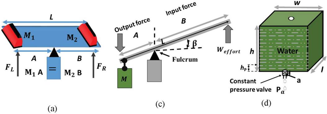
Figure 1 (a) Law of lever, (b) Second class lever, and (c) Water tank.
2 Mathematical Formulation of SCLPSAST
Archimedes’ lever law states, “The magnitude is in equilibrium at distances reciprocally proportional to their weights” as shown in Figure 1(a). The lever is equivalent to a beam. Three elements make up this device: the center or fulcrum, two weights, the one that creates movement and the one that causes it. The ideal mechanical advantage (IMA) of the lever is the ratio of input to output force (1). IMA of the fulcrum can determine the balance moments lever. A and B are the distances between the masses M (Left side mass) and M (Right side mass) of the lever with fulcrum L. The input and output forces F and F are shown in Figure 1(a).
| (1) |
2.1 Second-class Lever Principle
Second-class levers are defined as the input force required to produce a significant output force. The present invention defines M as the mass (kg) required to hold a PV module facing eastward at an angle .
| (2) | |
| (3) | |
| (4) |
Here, the work done by the area of arc is given in (2). The force is equal to Mg. By using (2) and (3) can get the required mass M to keep the PV panel to the east position (sunrise) at angle . Here, is mass of water, and M is mass of the tank.
2.2 Pressure at the Orifice
The SCLPSAST system is to maintain the PV module’s constant movement. So, the velocity of the discharge through the orifice for a predefined time ‘T’ (sec) should be constant. By using a constant pressure valve, it is possible to maintain a constant pressure output discharge of water at the orifice. The following section will explain this concept in detail. The illustration of water tank is given in Figure 1(c), where ‘h’ is height of water, is the bottom pressure and a is the area of the orifice. From the derivation of the expression for the pressure at the orifice, the time taken to drop the water level from ‘h’ to ‘’ must be calculated (the minimum height required for discharge through the orifice when the pressure level is less than the specified lower limit of the pressure valve). In (5), it is noted that the amount of water flowing through the orifice in time ‘T’ seconds is proportional to the amount of water leaving the tank through the orifice.
| (5) |
Here, is an area of the tank, T is time in seconds for the water to fall from ‘h’, and V is velocity through the orifice in m/s. The value of ranges from 0.61 to 0.69 and it is determined by the orifice’s shape and size.
From the Bernoulli’s principle, kinetic pressure at the orifice, and the water velocity through the orifice is m/s is given in (7). Here is the density of the fluid (kg/m). By using (5) and (7) can get the pressure at the orifice (pascal) in terms of discharge ‘T’ seconds.
| (6) | |
| (7) | |
| (8) |
3 Estimation of Sunrise and Sunset Time and Incident Solar Energy (H)
Many factors affect the estimation of sunrise, sunset, and incident solar energy () like time zone, latitude (), longitude (), collector orientation (collector tilt angle ()), time of the day (), sun declination angle (), time of the year and atmospheric conditions [9].
3.1 Solar Declination Angle ()
According to the earth’s centric viewpoint, a person standing at the equator would observe the sun moving in a definite pattern annually. During the summer solstice (Jun 21st), the sun reaches the extreme point in the northern hemisphere and the line assembly between the center of the sun and the earth would pass through the Tropic of Cancer thus making an angle of 23.45 with the equatorial plane. As days progress, the sun moves down, aligns itself along the equatorial plane on Sep 21st (equinox), and further moves down to cut the Tropic of Capricorn latitude in the southern hemisphere at an angle 23.45 on Dec 21st which is known as the winter solstice. Then it ascends and aligns with the equatorial plane again on Mar 21st (equinox). The cycle repeats every year and the earth-centric view is shown in Figure 2. angle differs from 23.45 to 23.45 [23]. The is as given in (9), where N is day number, which is 1 for Jan 1st and 365 for Dec 31st [27–29].
| (9) |
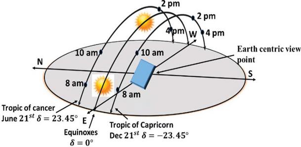
Figure 2 Earth-centric solar paths.
Figure 3 represents the solar geometry. The view direction is as though viewing the center of the earth from the east coordinate axis of the locale as well as the earth-centric coordinate system. The zenith axis can obtain using (10) [32].
| (10) |
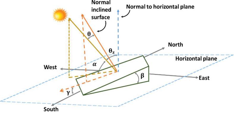
Figure 3 Solar geometry system.
3.2 Sunrise and Sunset Time
The sunrise and sunset time (11) and (12) can be obtained from (10). The sunrise angle is considered negative for the east and the sunset angle is considered positive for the west directions. To estimate the sunrise and sunset time for any day of the year, two values are to be calculated, the solar time correction (SC) and the solar declination angle (). SC is the minute’s difference between local time and solar time [30]. Sunrise and sunset are calculated based on standard time. The (), sunrise, and sunset time the throughout the year are shown in Figure 4. The sun hour angle can be obtained from (13). Here t is the specific time.
| (11) | |
| (12) | |
| (13) |
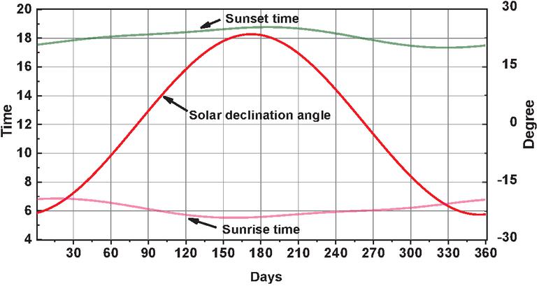
Figure 4 , sunrise, and sunset time.
3.3 Estimation of Incident Solar Energy ()
The daily incident solar energy MJ/m/day can be obtained on a horizontal flat plate on the earth’s surface is given in (14) [25, 26]. Here, is the mean solar constant equal to 1.37 kW/m [31]. In fact, the conventional PV is a fixed-position with a tilt angle ().
| (14) | ||
| (15) | ||
| (16) | ||
| (17) | ||
| (18) |
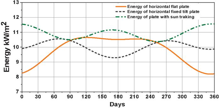
Figure 5 Annual incident solar energy.
The extraction of maximum energy in this case is possible only at the instant when the sun’s rays are usual to the PV surface. But in solar tracking system, and does not influence the system because the single-axis solar trackers always align parallel to the sun [32]. This is one of the benefits of a solar tracking system. Using (15), can be obtain the daily available energy () of a fixed tilt. By using Equations (16), (17), and (18) can be obtaining the solar radiation of horizontal surface , fixed tilt surface (), and single axis tracker (). Figure 5 shows the energy available of the horizontal flat plate, fixed tilted plate, and the plate while tracking the sun.
4 Illustration of SCLPSAST System
A and B are separated by 0.20 m and 0.37 m, respectively, by the fulcrum. The weight of the PV module is 2 kg. From Equation (1), it is calculated that the IMA is 1.6818 and the mass for holding the lever in the balance is 2.183 kg. Moreover, a mass of 2.29 kg is calculated from (4), with the PV panel being kept at an angle of 45 toward sunrise.
The design calculations of the SCLPSAST system are given below:
a. Calculation of weight
∙ Length m
∙ Length m
∙ IMA of the Fulcrum
∙ kg
∙ kg
∙ (Under balanced conditions)
∙ Sin ; where
∙ Total weight of water required to keep the PV pane through east direction at angle 45
b. Calibration of water flow rate
The SCLPSAST system needs to track the sun over the longest sunny day (13.24 hours). At the bottom of the container, the calibrated the flow rate at 2.883 ml/min by using a handle screw.
∙ Total water container dimension () 0.15 m * 0.15 m * 0.15 m 0.003375 litres.
∙ The exact amount of water which have to be filled in the container is 2.292 liters.
∙ Discharge through orifice:
Discharge through orifice per second
Table 2 Design parameters of boost converter
| Description | Parameters |
| Boost converter | L 1.0 mH, |
| kHz, IGBT – 1MBH60D100, | |
| Diode- RHRG30120, /5A |
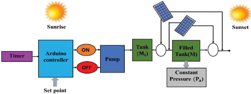
Figure 6 Functionality diagram.
5 SCLPSAST Functionality and Data Monitoring System
This analysis uses two identical PV set-ups with tracking and without tracking. To obtain the maximum power from the SCLPSAST and FSA system, MPPT (Perturb and Observe) DC-DC boost converters are used [33–35]. Table 2 provides the design parameters for the DC-DC boost converter. The system specifications of the PV module, water tank, and solar water pump used in the experimental are presented in Tables 3 and 4. The FSA system (ref Figure 10(d)) is immovable with a tilt angle of 11 facing south.
Table 3 Technical specification of water tank and water pump
| Name of the Parameter | Value |
| Water tank | |
| Liters | 3000 ml |
| Empty tank weight | 200 g |
| Length of tank | 0.15 m |
| Width of tank | 0.15 m |
| Height of tank | 0.15 m |
| Constant pressure valve specification | 0.01 to 0.8 MPa |
| Solar water pump controller | |
| DC Voltage | 12 V |
| Pump power | 8 W |
| Height max | 5 m |
| Flow | 5 L/min |
| Timer | DS3231 |
| Arduino controller | Arduino Uno |
Table 4 Technical specification of solar panel
| Name of the Parameter | Value |
| Maximum power rating (P) | 20 W |
| Number of cells in series | 36 |
| Open circuit voltage, (V) | 21.6 V |
| Maximum power voltage (V) | 17.2 V |
| Short circuit current (I) | 1.31 A |
| Maximum power current (I) | 1.16 A |
| Mass of solar panel () | 1.5 Kg |
| Length of the solar panel () | 570 mm |
| Width of the solar panel (W) | 330 mm |
| Height of solar panel (D) | 11 mm |
| Specifications total angle () | 86 |
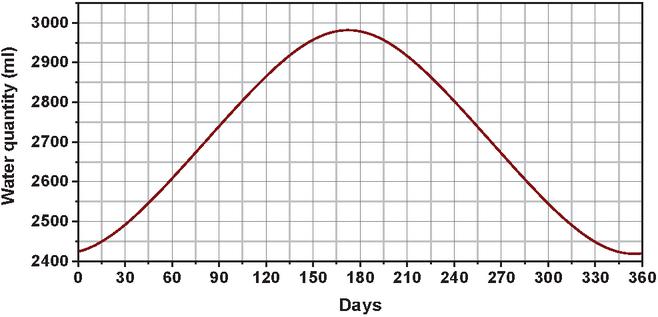
Figure 7 Water quantity required throughout year.
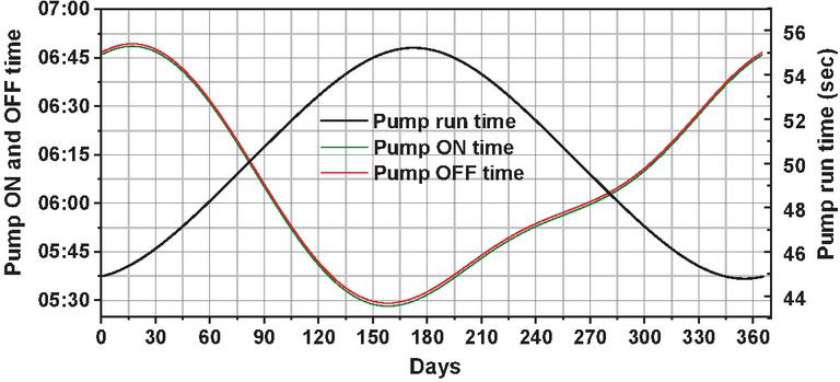
Figure 8 Pump ON and OFF time, and run time.

Figure 9 Sun hour versus SCLPSAST PV module angle, changes of with water height.

Figure 10 SCLSAST system (a) Morning, (b) After noon (c) Evening, and (d) FSA system.
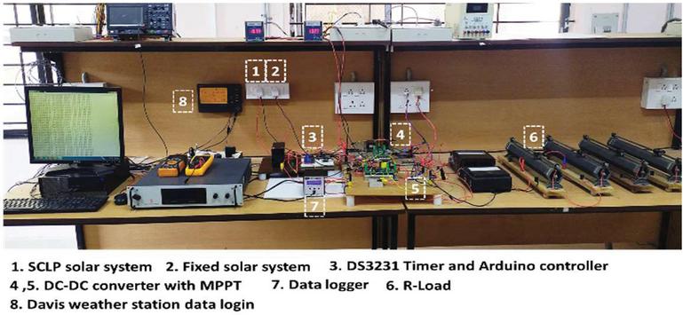
Figure 11 Data monitoring system and DC-DC converter of SCLPSAST and FSA.
SCLPSAST will begin functioning every morning before sunrise for the entire year, and it will keep working from sunrise until sunset. It should be noted that the solar panel’s starting position before the day’s sunrise will be in the West (Sunset). Based on control signal from the timer circuit, the Arduino microcontroller communicates with the pump. Just before sunrise, the pump is turned ON and automatically fills water in the tank. Once water is filled in the tank to the required level, the DC pump turns OFF automatically. All of these processes are managed by a predefined programmed that is created, using Arduino controller. Functional work diagram is given in Figure 6. The water required throughout the year is shown in Figure 7. ON and OFF time of the pump, and the pump run time is shown in Figure 8. The variation of the curves representing PV module angle and water height in the tank from the sun hour angle curve plotted against time is shown in Figure 9.
At the starting time, i.e. sunrise, the position of the PV module is at an angle as shown in Figure 10(a). The constant pressure value is provided at the base of the water tank. Water starts discharging through the constant pressure value at a constant velocity once the tank is filled to a certain level. It reduces the weight of the tank and allows the solar panel to track the sun. SCLPSAST system, during solar noon and sunset positions, are shown in Figure 10(b) and 10(c) respectively. The data monitoring system and DC-DC converters of the SCLPSAST and FSA system are shown in Figure 11.
Most stainless steel needle valves feature a significant pressure drop from the inlet to the outlet, which makes them ideal for low flow rates. All fluid control applications are uses needle valves because they can precisely control flow rate. Threads in these valves allow the plunger’s tapered end to be precisely positioned away from the valve seat to control the flow rate accurately. Its tapered end raises and lowers as it spins, opening and closing a constant pressure valve. By varying the plunger setting, the flow rate can be adjusted between zero and maximum.
The holding structure of the water container prevents north-south movement, so the wind does not significantly affect the container in this direction. Parallelogram diagonal control structures can be used to reduce east-west wind energy’s impact on water containers. Equation (19) can be used to determine the shape of the parallelogram diagonal control structure as shown in the Figure 12.
| (19) |
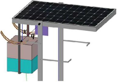
Figure 12 Parallelogram diagonal control structures for SCLPSAST system.
SCLPSAST controls the liquid pumping unit, which aligns the PV module with the sun. In addition to forecasting the sun’s position, it also predicts the time of day. The program for controlling the liquid pumping unit to fill the water holding unit to a preset threshold volume is also stored in memory. This program, the panel is positioned according to the sun’s position. The real-time weather parameters like solar irradiation, air and ambient temperature, et, have been taken from the Davis Vantage Pro2 (6152C) weather station.
6 Performance Evaluation
SCLPSAST and FSA systems are evaluated and compared in terms of performance indices such as module efficiency () and energy improvement (EI). The power curve of both SCLPSAST and FSA systems for a typical day (28-01-2022) and a partly cloudy day (24-02-2022) is shown in Figures 13 and 14, respectively. From the figures, it is detected that the SCLSAST system generates 70% to 1.61% excess power compared to the FSA system. The minimum excess power is obtained, during the noon time zone from 11.30 am to 1.30 pm, when the SCLPSAST system’s PV panel is in a horizontal position facing the sun directly.

Figure 13 Power curve on typical day (28-01-2022).
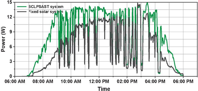
Figure 14 Partly cloudy day (24-02-2022).

Figure 15 Daily energy generation.
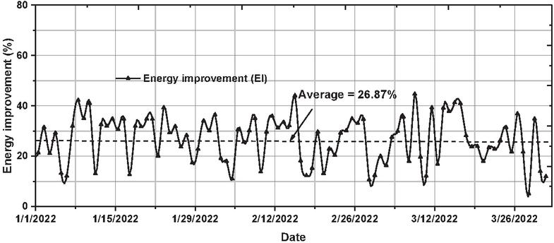
Figure 16 Percentage of energy improvement.
The energy improvement (EI) and efficiency () of SCLPSAST system and FSA system is calculated using (20) and (21), respectively. Here, P is the PV panel power, Gt (W/m) is the solar irradiation, A is the module area (0.19 m), and NPV is number of PV modules in the arrangement. Here, NPV 1. and E are the generated energy in Watt-hour for SCLPSAST and FSA systems, respectively.
| (20) | |
| (21) |
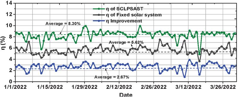
Figure 17 Efficiency.
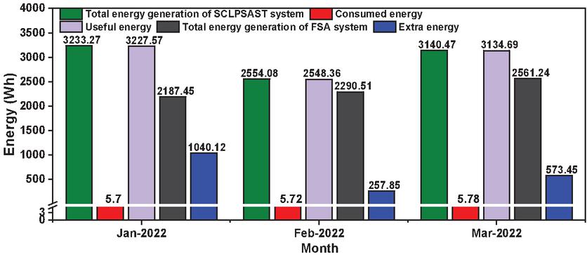
Figure 18 Monthly energy generation.
The plots of energy generated, energy improvement, and efficiency for a duration of 3 months are shown in Figures 15, 16, and 17 respectively. From these plots observed that the SCLPSAST system has an average energy improvement of 26.87% compared to the FSA system. The useful energy generation after deducting the expended energy consumed by support accessories of SCLPSAST system such as Adruino controller and pump is shown in Figure 18. Therefore, the total energy generationj of the SCLPSAST and FSA system during testing period is found to be 8.92 kWh and 7.03 kWh, respectively.
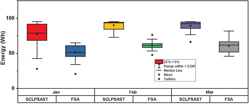
Figure 19 Box chart of statistical parameters.
7 Statistical Evaluation
The statistical performance characteristics is observed during testing the effectiveness of the SCLPSAST system over FSA system. The box chart shown in Figure 19 compares the statistical parameters of daily generated energy for three months namely, mean, standard deviation, median, quadrille, etc. A hypothesis test is also carried based on daily values to demonstrate the SCLPSAST system’s efficiency. Table 5 shows the T-test hypothesis parameters observed over a typical three months. The following conclusions are drawn from the T-test. SCLPSAST system’s average daily solar generation is 27.68 Wh more than the FSA system. The test evaluates the uncertainty in calculating the genuine difference of daily energy generation between the mean of SCLPSAST and FSA systems. There is a 95% of assurance that the true improvement is caluculated as 26.87%. Moreover, there are no unexpected data points that indicate a significant influence on the results.
Table 5 Hypothesis testing (Jan to Mar). Null Hypothesis . Alternative hypothesis
| Parameters | SCLPSAST | FSA | Difference |
| N | 90 | ||
| Mean | 85.45 | 57.76 | 27.68 |
| SD | 12.66 | 9.71 | 6.33 |
| SEM | 1.32 | 1.01 | 0.66 |
| Median | 91.28 | 59.74 | 28.36 |
| T-statistics | 41.91 | ||
| DF | 91 | ||
| Probability | 2.71E-61 | ||
8 Conclusion
Solar PV trackers will play an important role in PV energy generation worldwide in the coming days. The SCLPSAST system is a solar tracker that runs in chronological order. It follows the sun regardless of weather conditions. One of the advantages of the SCLPSAST system is the requirement of very low energy of its support accessories and no external motor is required. The SCLPSAST is simple to use and easy to implement, requiring less maintenance. The water is used as the working fluid and is not wasted. The SCLPSAST is compared to a conventional FSA system with the same rating. In comparison to the FSA system, there is a significant energy improvement of 26.87%. Moreover, the SCLPSAST is efficient in tracking the sun and has guaranteed improvements in energy produced which is validated using hypothesis testing.
Acknowledgement
This work is supported by the Government of India, Department of Science and Technology (Technology Mission Division-Water and Clean Energy) F. No. DST/TMD/CERI/RES/2020/35(G).
References
[1] Nan, J, ‘Key Technology Optimization and Development of New Energy Enterprises of Photovoltaic Power Generation’, Distributed Generation & Alternative Energy Journal, vol. 37(1), pp. 117–128, 2021. Available: https://doi.org/10.13052/dgaej2156-3306.3716.
[2] Dutta, A., Biswas, J, Roychowdhury, S, Neogi, S, ‘Optimum Tilt Angles for Manual Tracking of Photovoltaic Modules.’ Distributed Generation & Alternative Energy Journal, vol. 31(02), pp. 7–35. Available: https://doi.org/10.13052/dgaej2156-3306.3121.
[3] Mohammad, S. S., and Iqbal, S. J, ‘Optimization and Power Management of Solar PV-based Integrated Energy System for Distributed Green Hydrogen Production’, Distributed Generation & Alternative Energy Journal, vol. 37(4), pp. 865–898, 2022. Available: https://doi.org/10.13052/dgaej2156-3306.3741.
[4] Iqbal, S. J., and Mohammad, S. S, ‘Power Management, Control and Optimization of Photovoltaic/Battery/Fuel Cell/Stored Hydrogen-Based Microgrid for Critical Hospital Loads’, Distributed Generation & Alternative Energy Journal, vol. 37(4), pp. 1027–1054, 2022. https://doi.org/10.13052/dgaej2156-3306.3747.
[5] Finster C. El Heliostato de la Universidad Santa Maria. Scientia, vol. 119, pp. 5–20, 1962.
[6] A Sun-tracking system. Applied Energy., vol. 79, pp. 345–354. 2004. Available: https://doi.org/10.1016/j.apenergy.2003.12.004.
[7] Clifford M.J. and Eastwood D, ‘Design a novel passive solar tracker’, Solar Energy. vol. 77, pp. 269–280. 2004. Available: https://doi.org/10.1016/j.solener.2004.06.009.
[8] B. J. Huang. and F. S. Sun, ‘Feasibility study of one axis three positions tracking solar PV with low concentration ratio reflector’, Energy Convers. Manag., vol. 48, no. 4, pp. 1273–1280. 2007. Available: DOI: 10.1016/J.ENCONMAN.2006.09.020.
[9] N. Mohammed and T. Karim, ‘Design and implementation of hybrid automatic solar tracking system’, Int. J. Electr. Power Eng., vol. 6, no. 3, pp. 111–117. 2012. Available: https://doi.org/10.1115/1.4007295.
[10] M. Mahendran. H. L. Ong. G. C. Lee. and K. Thanikaikumaran, ‘An experimental comparison study between single-axis is tracking and fixed photovoltaic solar panel efficiency and power output: Case study in east coast Malaysia’, in Sustainable Development Conference. Bangkok. Thailand, 2013. Available: http://umpir.ump.edu.my/id/eprint/3797.
[11] B. Huang. Y.-C. Huang. G.-Y. Chen. P.-C. Hsu. and K. Li, ‘Improving solar PV system efficiency using one-axis 3-position Sun tracking’, Energy Procedia. vol. 33, pp. 280–287. 2013. Available: https://doi.org/10.1016/j.egypro.2013.05.069.
[12] I. Abadi. A. Soeprijanto. and A. Musyafa, ‘Design of single axis solar tracking system at photovoltaic panel using fuzzy logic controller’, in 5th Brunei International Conference on Engineering and Technology (BICET 2014). 2014. Available: https://ieeexplore.ieee.org/document/7120264.
[13] R. A. Ferdaus. M. A. Mohammed. S. Rahman. S. Salehin. and M. Abdul Mannan, ‘Energy efficient hybrid dual axis solar tracking system’, J. Renew. Energy. pp. 1–12. 2014. Available: https://doi.org/10.1155/2014/629717.
[14] G. C. Lazaroiu, M. Longo, M. Roscia. and M. Pagano, ‘Comparative analysis of fixed and Sun tracking low power PV systems considering energy consumption’, Energy Convers. Manag. vol. 92, pp. 143–148. 2015. Available: https://doi.org/10.1016/j.enconman.2014.12.046.
[15] M. Yılmaz and F. Kentli, ‘Increasing of electrical energy with solar tracking system at the region which has Turkey’s most solar energy potential’, Clean Energy Technol. vol. 3, no. 4, pp. 287–290. 2015. Available: DOI: 10.7763/JOCET.2015.V3.210.
[16] A. Cammarata, ‘Optimized design of a large-workspace 2-DOF parallel robot for solar tracking systems’, Mech. Mach. Theory. vol. 83, pp. 175–186. 2015. Available: DOI: 10.1016/j.mechmachtheory.2014.09.012.
[17] J. Parmar. N. Parmar. S. Gautam, ‘Analysis and implementation of passive solar tracking system’, International Journal of Emerging Technology and Advanced Engineering. vol. 5(1), pp.138–145. 2015. Available: https://www.semanticscholar.org/paper/Passive-Solar-Tracking-System-Parmar-Parmar/79affcd91f1088d9f3ad1f48323aaa0962b218a7.
[18] K. K. N. V. Subramaniam. and M. E, ‘Power analysis of non-tracking PV system with low power RTC based sensor independent solar tracking (SIST) PV system’, Mater. Today Proc. 2016. Available: https://doi.org/10.1016/j.matpr.2017.11.185.
[19] A. S. C. Roong and S.-H. Chong, ‘Laboratory-scale single axis solar tracking system: Design and implementation’, Int. J. Power Electron. Drive Syst. vol. 7, no. 1, pp. 254–264. 2016. Available: DOI: 10.11591/IJPEDS.V7.I1.PP254-264.
[20] Basnayake Jayathilaka. Amarasinghe, Attalage RA. Jayasekara AGBP, ‘Smart solar tracking and on-site photovoltaic efficiency measurement system’, Moratuwa Eng Res Conf (MERCon). pp. 54–9. 2016. Available: DOI: 10.1109/MERCon.2016.7480115.
[21] Shinya Obaraa. Kazuhiro Matsumurab. Shun Aizawac. Hiroyuki Kobayashid. Yasuhiro Hamadae. and Takanori Sudaf, ‘Development of a solar tracking system of a nonelectric power source by using a metal hydride actuator’, Solar Energy. vol. 158, pp. 1016–1025. 2017. Available: https://doi.org/10.1016/j.solener.2017.08.056.
[22] Mostefa Ghassoul, ‘Single-axis automatic tracking system based on PILOT scheme to control the solar panel to optimize solar energy extraction’, Energy Reports. vol. 4, pp. 20–527. 2018. Available: https://doi.org/10.1016/j.egyr.2018.07.001.
[23] Hossein Mousazadeh. Alireza Keyhani. Arzhang Javadi. Hossein Mobli. Karen Abrinia. Ahmad Sharifi, ‘A review of principle and Sun-tracking methods for maximizing solar systems output’, Renewable and Sustainable Energy Reviews, vol. 13, pp. 1800–1818. 2009. Available: https://doi.org/10.1016/j.rser.2009.01.022.
[24] Single Axis Solar Tracking System And Method Thereof, by Sishaj P Simon. K. Sundareswaran. P. Srinivasarao Nayak. et., 07/04/2022, Patent Number:394395.
[25] Camelia Stanciu. Dorin Stanciu, ‘Optimum tilt angle for flat plate collectors all over the World A declination dependence formula and comparisons of three solar radiation models’, Energy Conversion and Management. vol. 81, pp. 133–143. 2014. Available: http://dx.doi.org/10.1016/j.enconman.2014.02.016.
[26] Basharat Jamil. Evangelos Bellos, ‘Development of empirical models for estimation of global solar radiation exergy in India’, Journal of Cleaner Production. vol. 207, pp. 1–16. 2019. Available: https://doi.org/10.1016/j.jclepro.2018.09.246.
[27] Akhlaghi. S. Sangrody. H. Sarailoo. M, ‘Efficient operation of residential solar panels with determination of the optimal tilt angle and optimal intervals based on forecasting model’, IET Renew. Power Gener. vol. 11, pp. 1261–1267. 2017. Available: DOI: 10.1049/iet-rpg.2016.1033.
[28] J. The role of solar-radiation climatology in the design of photovoltaic systems’ Part II-1-A, McEvoy’s handbook of photovoltaics. Elsevier Academic Press. United Kingdom, 3rd Edn. pp. 601–670. 2018. Available: https://doi.org/10.1016/B978-185617390-2/50004-0.
[29] Kalogirou. S.A., ‘Environmental characteristics, Solar Energy Engineering: Processes and Systems Chapter II’, Elsevier Academic Press, United Kingdom 2014, pp. 51–123. Available: https://www.elsevier.com/books/solar-energy-ngineering/kalogirou/978-0-12-397270-5
[30] Brownson. J. R. S., Sun-Earth Geometry. Solar Energy Conversion Systems. pp. 135–178. 2014. Available: https://doi.org/10.1016/B978-0-12-397021-3.00006-5.
[31] S. Bhattacharjee. S. Bhakta, ‘Analysis of system performance indices of PV generator in a cloudburst precinct’, Sustainable Energy Technologies and Assessments. vol. 4, pp. 62–71. 2013. Available: http://dx.doi.org/10.1016/j.seta.2013.10.003.
[32] M. A. Danandeh. S. M. Mousavi G, ‘Solar irradiance estimation models and optimum tilt angle approaches: A comparative study’, Renewable and Sustainable Energy Reviews. vol. 92, pp. 319–330. 2018. Available: https://doi.org/10.1016/j.rser.2018.05.004.
[33] Praveen Kumar, T. Subrahmanyam, N., and Sydulu, M, ‘Power Management System of a Particle Swarm Optimization Controlled Grid Integrated Hybrid PV/WIND/FC/Battery Distributed Generation System, Distributed Generation & Alternative Energy Journal, vol. 36(2), pp. 141–168, 2021. Available: https://doi.org/10.13052/dgaej2156-3306.3624.
[34] Puthusserry, G. V, Sundareswaran, K., Simon, S. P, and Krishnan, G. S. ‘Maximum Energy Extraction in Partially Shaded PV Systems Using Skewed Genetic Algorithm: Computer Simulations, Experimentation and Evaluation on a 30 kW PV Power Plant’, Distributed Generation & Alternative Energy Journal, vol. 37(06), pp. 1773–1796. Available: https://doi.org/10.13052/dgaej2156-3306.3763.
[35] Sutikno, T, Subrata, A. C, and Jusoh, A, ‘A New FL-MPPT High Voltage DC-DC Converter for PV Solar Application’, Distributed Generation & Alternative Energy Journal, Vol. 37(05), pp. 1527–1548. Available: https://doi.org/10.13052/dgaej2156-3306.37510.
Biographies

Krishna Kumba received the B.Tech. degree in electrical and electronics engineering from JNTU Hyderabad, India, in 2008; and the M. Tech. degree in the control system, from National Institute of Technology Kurukshetra, Haryana, India, in 2010. Currently, he is pursuing a Ph.D. degree in electrical and electronics engineering from the National Institute of Technology, Tiruchirappalli, Tamil Nadu, India. His research interests include power system planning and reliability. renewable energy systems.

Sishaj P. Simon was born in India. He received the B.Eng. degree in electrical and electronics engineering, the M.Eng. degree in applied electronics both from Bharathiar University, Coimbatore, Tamil Nadu, India, in 1999 and 2001, respectively, and the Ph.D. degree in power system engineering from Indian Institute of Technology (IIT), Roorkee, Uttarakhand, India, in 2006. Currently, he is an Associate Professor with the Department of Electrical and Electronics Engineering, National Institute of Technology (NIT) (formerly Regional Engineering College), Tiruchirappalli, Tamil Nadu, India. His research interests include the area of power system operation and control, power system planning and reliability, artificial neural networks, fuzzy logic systems, and application of meta-heuristics, and intelligent techniques to power systems.

Kinattingal Sundareswaran was born in Pallassana, Kerala, India, in 1966. He received the B.Tech. (Hons.) degree in electrical and electronics engineering and the M.Tech. (Hons.) degree in power electronics from the University of Calicut, Calicut, Kerala, India, in 1988 and 1991, respectively, and the Ph.D. degree in electrical engineering from Bharathidasan University, Tiruchirappalli, Tamil Nadu, India, in 2001. From 2005 to 2006, he was a professor with the Department of Electrical Engineering, National Institute of Technology, Calicut, Kerala, India. He is currently a Professor with the Department of Electrical and Electronics Engineering, National Institute of Technology, Tiruchirappalli, Tamil Nadu, India. His research interests include power electronics, renewable energy systems, and biologically inspired optimization techniques.

Panugothu Srinivasan Rao Nayak was born in Perikapadu, Guntur, Andhra Pradesh, India, in 1979. He received the B.Tech. degree in electrical and electronics engineering from Bapatla Engineering College (BEC), Bapatla, Guntur, in 2001; the M.Tech. degree in energy systems from Jawaharlal Nehru Technological University (JNTU), Hyderabad, Telangana, India, in 2006; and the Ph.D. degree in electrical engineering from the National Institute of Technology, Tiruchirappalli, Tamil Nadu, India, in 2014. Currently, he is an Assistant Professor with the Department of Electrical and Electronics Engineering, National Institute of Technology. His research interests include power electronics and drives, biologically inspired optimization techniques, and wireless power transfer systems.
Distributed Generation & Alternative Energy Journal, Vol. 38_5, 1559–1584.
doi: 10.13052/dgaej2156-3306.3859
© 2023 River Publishers