An Efficient Libed and GBLRU-Based Solar Panel Hotspot Detection System Using Thermal Images
P. Pradeep Kumar1,* and M. Rama Prasad Reddy2
1EEE Department JNTUA, Anantapuram, Andhra Pradesh, India
2EEE Department, G. Pullaiah College of Engineering and Technology, Kurnool, Andhra Pradesh, India
E-mail: poluripradeep238@gmail.com; mrpreddyeee@gpcet.ac.in
*Corresponding Author
Received 25 February 2023; Accepted 06 September 2023; Publication 02 November 2023
Abstract
In the Photovoltaic (PV) system, monitoring, assessing, and detecting the occurred faults is essential. Autonomous diagnostic models are required to examine the solar plants and to detect the anomalies within these PV panels since the prevailing hotspot detection models were unable to detect the faults rapidly and consistently. A novel Log Inverse Bilateral Edge Detector (LIBED) and Gated Bernoulli Logmax Recurrent Unit (GBLRU)-centered Solar Panel (SP) hotspot detection scheme is proposed in this research that analyzed the operating PV module’s thermal images. Images are applied for the image processing steps prior to hotspot detection. By utilizing the Contrast Limited Adaptive Histogram Equalization (CLAHE) model, the image’s contrast has been augmented in the image processing step.
The alpha () Modified Histogram Blending (MHB) method is utilized to eliminate the outlier data available in the image. Subsequently, an effective LIBED contour detection method was utilized to detect the SP. Several features are extracted by utilizing the detected panels. Then, optimal features are chosen as of the extracted features by utilizing the Barnacles Mating Optimizer (BMO) algorithm. The GBLRU was utilized to predict the defective panels. The defective panels’ hotspots were isolated by utilizing the Haversine Self-Organizing Map (HSOM) model. The experimental evaluation of the proposed system’s performance is analyzed with the prevailing classifiers. The state-of-art methods were outperformed by the proposed GBLRU-based Hotspot detection system. The efficiency 94.34%, accuracy 97.23%, hot-spot detection rate 91.23% had been attained which were improved outcomes compared to existed models.
Keywords: PV panel defects, fault detection, diagnosis, thermal images, image processing, morphological operations.
1 Introduction
In order to lessen the harm caused by fossil fuel usage, several nations are currently interested in innovative and renewable energy sources (Charfi et al., 2018), (Lee et al., 2018). As a result, more and more attention was gained by solar power regarding the issue of global warming. There are primarily ‘2’ sorts of solar power generation as per the energy conversion form: PV power generation and thermal power generation (Chen et al., 2020). A popular renewable energy source that has the potential to supply clean, reliable, and expandable electricity in the future is solar PV technology (Kenu E. Sarah, 2020). Owing to the numerous benefits that PV energy systems provide, such as being a globally accessible energy source, being pollution-free, operating quietly, and so on, there has been an elevation in interest in these systems over the past 10 years (Mellit et al., 2018).
PV is termed as the conversion of light into electricity grounded on the photoelectric effect on semiconductor materials(Hernández-Callejo et al., 2019). In essence, it is a PV panel or module made of numerous single PV cells coupled in parallel and series to engender electricity utilizing solar energy (Ali et al., 2022). However, the panel’s efficiency declines when abnormalities like hot spots are present. A hotspot is a flaw in a Photovoltaic Module (PCM) that prevents the PVM’s typical operation. Numerous things might cause hot spots to emerge, including cracked modules, faulty solder joints, accidental connections, shading, and soiling (Afifah et al., 2020). There is a significant loss of power in the poor cell when this happens. Local overheating or hotspots are caused by the local dissipation of power in a petite area. Continuous yield losses could result from this, and hotspots could even catch fire in the worst-case conditions (Salazar and Macabebe, 2016).
Therefore, to safeguard Photovoltaic Systems (PVS) components (modules, batteries, and inverters) specifically, PVM from harm and to eradicate potential fire threats, Fault Detection and Diagnosis (FDD) for PV plants is an essential task. The operating process employing thermographic cameras in existing technologies, particularly hot-spot identification, is well-defined and applicable to PV installations. Since the detection method is manual, it is typically a time-consuming and costly operation (Salamanca et al., 2017). To automatically detect hotspots in SPs, the proposed approach suggested an algorithm known as Log Inverse Bilateral Edge Detector (LIBED) and Gated Bernoulli Logmax Recurrent Unit (GBLRU).
1.1 Problem Definition
There aren’t many research studies that have evaluated the difficulties and effectiveness of the techniques utilized to classify alongwith identify various defect classes in PV modules. However, the prevailing research model’s disadvantages are described below,
• The hotspots on the PV panels are evaluated, classified, and identified utilizing the current Machine Learning (ML) technique, which employs a histogram of gradient attributes to categorize the hotspots. However, this method only partially classifies the system’s various PV complications.
• Since the colour space was diminished from 3 to 2 dimensions, it employs RGB to LAB colour conversion, which diminishes the algorithm’s computational cost. However, these outcomes with a significant fluctuation in the cluster can occasionally lead to over-enhancement issues.
• Prevailing methods for detecting hotspots in SPs involve severalML-centered prediction models, which failed to engender the anticipated results.
These are the main drawbacks that motivate to propose a methodology that elevates hotspot detection using thermal images. Some research objectives in the proposed methodology are enlisted as follows,
• To suggest an effective pre-processing algorithm for thermal image colour correction.
• To propose an efficient technique for edge detection without over-smoothening of images.
• To propose a novel classifier for the classification of normal and defective panels.
• To propose an innovative algorithm for hotspot detection.
The PV arrays are most prominent equipment to the present power generation applications. In this research, detecting the solar hot-spots even less solar energy illumination environment. The LIBED AND GBLRU technologies has been used to recognize the solar hot spots for PV accurate functioning.
This remaining paper is categorized as follows: the work correlated to this paper is represented in Section 2. The methodology which is proposed is demonstrated briefly in Section 3. The proposed work’s outcomes and discussion are illustrated in Section 4, and lastly, the conclusion has been drawn from the whole work in Section 5.
2 Literature Survey
Díaz et al. (2020) utilized thermal images acquired by Unmanned Aerial Vehicles (UAVs) to establish SP detection within complicated backgrounds. The model utilized to detect SPs comprised of the following steps: the first model was grounded on edge detection and classification while the second model was grounded on training a region-centered Convolutional Neural Network (CNN) to recognize a panel. When analogized to some other techniques, a better outcome was illustrated by the experiential outcomes. But, the correction was required for the lens distortion visible in the thermal images, which was the disadvantage.
Ali et al. (2020) projected a hybrid features-based Support Vector Machine (SVM) model for hotspot detection and PV panel classification utilizing an Infrared (IR) thermography model. RGB texture, Histogram of Oriented Gradient (HOG), and Local Binary Pattern (LBP) are available inthe hybrid feature vector. To classify the obtained thermal images of PV panels into ‘3’ diverse classes like healthy, non-faulty hotspots, and faulty, the SVM algorithm was employed. The experiential outcomes exposed that better training and testing accuracy was obtained by the presented hybrid features with SVM than other ML algorithms with lesser computational complexity and storage space. However, owing to higher training time, the model was not perfectly executed.
Pierdicca et al. (2020) propounded an artificial intelligence system grounded on Deep Learning (DL) for anomaly cell detection in PV images acquired as of UAVs equipped with a thermal IR sensor. The UAV-centered inspection system, the Mask Region-centered CNN (Mask R-CNN) architecture, and the Deep Neural Networks (DNNs)-based solution were the ‘3’ components that comprised this framework. The anomalous cells in PV plants were monitored and identified by utilizing an intelligent inspection system grounded on UAVs. To perform object detection along with instance segmentation simultaneously, R-CNN was adopted thereby making it beneficial for the automated inspection task. As a backbone for feature extraction, CNN was used as DNN for image classification. But, more time was consumed for the introduced approach’s process and further equipment was required.
Niazi et al. (2019) introduced a non-invasive ML-centered fault diagnosis model for PVM. Rather than a binary classifier, the multi-class density-based classifier such as nBayes classifier was utilized for training the algorithm. Digital image processing techniques were utilized by the presented algorithm. The damage and/or degradation in PV modules were identified reliably by the Naive Bayes (nBayes) classifier. Higher accuracy along with the low computational cost was attained by the methodology when analogized to baseline models. The detection and classification of PVM were accurately elevated by implementing segmentation techniques that could further extend the model.
Huerta Herraiz et al. (2020) developed a model to locate hot spots along with recognize panels to detect them. To engender a robust detection structure, two novel region-centered CNN were unified. To offer a response to the panel condition monitoring, the combination of thermography and telemetry data was the major contribution. During the inspection, the data were obtained and processed autonomously to permit fault detection. For the autonomous detection and localization of solar trackers, the outcomes exhibited that the model was sufficient with better accuracy and precision. However, the faulty PV panel’s correct localization was not guaranteed by this methodology owing to the positioning error.
Et-Taleby et al. (2020) provided Fault Detection (FD) for the PV field grounded on k-means, elbow, and average silhouette techniques viathermal image segmentation. Grounded on the thermal image clustering via the K-means algorithm, the damaged area in PV fields is detected and located precisely by the suggested work. To identify and detect the faulty panels precisely, the outcomes illustrated that an excellent outcome was provided by the K-means algorithm and elbow method. The k-means algorithm’s main drawback was that there was trouble in clustering data where clusters are of varying size and density.
Menéndez et al. (2018) introduced PVM diagnosis utilizing artificial vision approaches for artifact minimization. A portable ground-centered system that has the ability to detect along with classifies hotspots associated with PVM failures were tested here. As of the panel structure, the system is characterized by 3-Dimensional thermal information to detect along with classifying hotspots. The experiential outcomes illustrated that the output quality was grounded on the classification accuracy along with the module segmentation in the RGB camera readings and the thermal image, respectively. However, the method should be closely probable to the measured data in the field by pondering the uncertainties and actual measurement conditions.
Wlodarczak (2019) presented DL-centered PVFD techniques utilizing thermal images acquired as of UAV equipped with IR sensors. To detect defective panels on large solar plantations, the ‘3’ most accurate segmentation models implemented were the DeepLabV3+, Feature Pyramid Network (FPN), and U-Net. The attained outcomes exposed that the conventional image segmentation approaches were outperformed by the DL-centred segmentation models significantly. However, when there were consistent or more than 2 defective SPsin one image, the segmentation quality was not smooth.
Balasubramani et al. (2020) suggested a new Thermal Pixel Counting (TPC) algorithm in FD grounded on ‘3’ thermal profile index values. Utilizing FLIR, real-time experiential testing was performed. Owing to the new input patterns’ learning ability, the experiential outcomes articulated that better classification accuracy was obtained by the CF when analogized with other models. Hence, owing to environmental temperature conditions and thermal camera noise, more detailed investigations were still needed by the introduced approach.
Fernández et al. (2020) suggested a robust detection, classification, and localization of defects in large PV plants centered on UAV and IR thermography. A fully automated framework for the detection, classification, and thermal defects geo positioning in the PVMs was provided here. By pondering the panel corner, the introduced approach was centered on the amalgamation of adaptive thresholding and the correction of perspective distortion. For an appropriate automated PV plants’ thermal inspection, the experimental outcomes exhibited the provided system’s utilization. However, major challenges like the cost and time of detecting PVM defects with their classification and exact localization within the solar plant were signified by the cost-effective model’s implementation to scan along with check huge PV plants.
Jeong et al. (2020) introduced an image processing framework that detected the module engendering the hot spots in the solar module autonomously. The Maximally Stable Extremal Regions (MSER) model was utilized to derive the area of interest by utilizing the in-range functions to retrieve feature points employing the PVM’s blue color. The experiential outcomes illustrated that a better match betwixt the thermal image and the visible image along with the accuracy of implementing the MSER algorithm was attained than the prevailing models. However, testing on large-scale PV power stations was lacking here.
Wang et al. (2021) suggested automatic anomaly detection for PV systems utilizing thermography imaging together with low-rank matrix decomposition. The algorithm utilized in this technique was the Robust Principal Component Analysis (RPCA), which has the ability to isolate sparse corrupted anomalous components as of a low-rank background. The image processing and statistical ML techniques were amalgamated in this framework. The outcomes exhibited that significant anomalies were successfully detected by this algorithm. However, deriving the conditions on signal types along with deformation groups was lacking in this system.
Henry et al. (2020) provided an autonomous detection system for deteriorated PV Mutilizing a drone with a thermal camera. An automated drone flight path planning algorithm was presented by this approach to manage the drone autonomously. The need for manual drone control that detects along with locating the faulty PVM in large-scale PV power stations was eliminated by this algorithm. To process RGB and thermal images, an image processing algorithm was utilized by this system for fault detection. The model’s outcomes suggested that the faulty modules were accurately detected and located by the presented model. However, the detected error sources need to be recognized manually.
Akram et al. (2020) presented an autonomous PVM defects detection in IR images with isolated DL and develop-model transfer DL techniques. The network was trained by utilizing an IR images dataset that was gathered. IR images of normal operating and defective modules were comprised in this dataset. The experiential outcomes exhibited that better accuracy and prediction time was attained by the suggested model. However, the wrong decisions were caused by the small image samples at the border of clearly noticeable normal operating and defective PVM images.
Fonseca Alves et al. (2021) introduced an automatic PVM fault classification utilizing CNN. To elevate the introduced CNN performance to classify anomalies betwixt 11 diverse classes the impact of data augmentation techniques was examined in PVM via thermographic images in an unbalanced dataset. Better power reduction levels were obtained by the outcomes of this study as a whole. Yet, accuracy was still lacking in this approach.
3 Proposed Solar Panel Hotspot Detection System
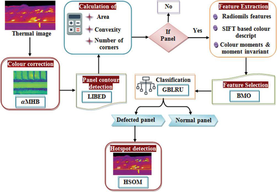
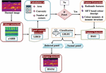
A novel algorithm is proposed in this paper for hotspot detection in SPs. Panels detection, detected panel classification, and localizing the SP’s hotspot were the ‘3’ steps undergone in the proposed model. Figure 1 proffers the proposed methodology’s block diagram.
Figure 1 Block diagram of the proposed methodology.
3.1 Color Correction
The obtained thermal images are processed by the proposed system. The input images are transformed initially into grayscale images. And, it undertakes the alpha () Modified Histogram Blending (MHB) algorithm, which is the image processing algorithm. However, the generation of images with low contrast along with loss in the textural characteristics was implied by the normalization in cases where the sun reflection hotspots occur. Thus, it is proposed to eliminate the outlier data by utilizing the MHB technique where the equalized image is multiplied by the alpha () value to prevent the subtleties loss in the image. The alpha value is randomly chosen betwixt a few ranges that are unsuitable for all images. By the equalized image’s minimal pixel value,the alpha value is chosen in the proposed work. Here, the CLAHE Algorithm is employed to execute the image equalization. Rather than the whole image, CLAHE functions on tiles which are the petite regions in the image. To eliminate the artificial boundaries, bilinear interpolation is utilized to merge the neighboring tiles. Hence, the thermal images’ color correction is as follows.
Let the set of input images may be represented as , . The input images are partitioned into a number of regions to execute histogram equalization. A histogram is computed for every region and a clip limit was utilized to limit the contrast.
By clipping all histograms, the clip limit was utilized by limiting the contrast of each region to the desired level in this process. The clip limit can be acquired as,
| (1) |
Where, the total number of gray levels is illustrated as , the total number of pixels in the image is signified as , the factor ranges from to , the histogram slope’s maximum limit is notated as , and the clip limit is signified as . As the input image has a very low intensity, the image becomes brighter when is elevated. The histogram is made flatter by a larger .
The number of pixels higher than the clip limit is clipped and the remaining pixels are redistributed to each gray level. The probability of each pixel is computed as of the clipped histogram as,
| (2) |
The cumulative distribution function is derived corresponding to the image’s probability as,
| (3) |
Where, the gray levels’ total count is signified as , the cumulative distribution function is notated as , the probability of image pixel is illustrated by . Utilizing the transformation function , the input image’s intensity is mapped betwixt to in the cumulative distribution function as,
| (4) |
To obtain the equalized image , the neighboring regions are merged after enhancing the tiles’ contrast. For blending operation that normally engenders visual artifacts like ghosting, softened discontinuities, and reduced contrast, the equalized histogram is therefore rendered. To preserve the histogram, new colors that are not available in the input were introduced. The blending can be computed as,
| (5) | ||
| (6) |
Where, the output of blending operation is notated as , the input image’s histogram specification was illustrated by and is the exponential of value acquired from the equalized image’s minimum pixel value. Hence, the outcome of intensity conversion has been obtained as,
| (7) |
Where, the color correction procedure’s output image processed in the further section is specified as .
3.2 Panel Contour Detection
By employing an effective contour detection model named LIBED, the SP as of is detected after color correlation. To eliminate noise contents and edge-preserving, a non-linear technique named Bilateral Filter is utilized in the image processing field. The spatial kernel and the range kernel are the two kernel filters included in the bilateral filter for this. While the diversities in the intensities are smoothened by the range kernel, the image was smoothened by the spatial kernel grounded on the Gaussian function. However, for a few images, over-smoothening was caused by the spatial kernel while smoothening the image. In the spatial kernel function, an Inverse logarithmic function is applied to avoid over-smoothening. Utilizing the proposed LIBED algorithm, the edge detection is as follows.
The weighted sum of pixels in a local neighbourhood is computed when the image is applied for a bilateral filter. For substituting the pixel value, the weighted average is utilized for every neighboring pixel. The bilateral filter’s output can be estimated as,
| (8) |
Where, the normalization factor is notated as , the Inverse Logarithmic spatial and range kernel function is and , the pixel coordinates are signified as , and the intensity of pixels are signified as and . The Inverse Logarithmic spatial kernel function gauges the spatial distance as,
| (9) | ||
| (10) |
Where, the filtering amount for the image is notated as and . The impact of distant pixels is decreased by spatial weighting; whereas, the influence of pixels was decreased by the range weighting when their intensity values vary from . When sharp intensity alterations are maintained, it assures that for blurring; only those pixels with intensity values identical to the central pixel are pondered.
Erosion and dilation operations are executed subsequent to edge detection. To identify whether it is an SP or not, the convexity and the corners values are computed grounded on this area’s operation.
3.2.1 Erosion
The pixels on object boundaries were eliminated by erosion. In other words, the foreground objects were shrunk by it. For controlling this process, the structuring element which is a matrix of 1’s and 0’s is utilized. An image’s erosion is illustrated as,
Where, the erosion operation is illustrated as , the structuring element is notated as , the input image’s area and structuring element are denoted as and , and the structuring element’s pixel values and the input image is illustrated as .
3.2.2 Dilation
By adding the number of pixels to the boundaries of objects, the objects are grown or thickened by a dilation technique thereby the image is expanded as of its original shape. Grounded on the structuring element’s size and shape, the number of pixels should be added or eliminated as of the object to process the image. The dilation of an image is illustrated as,
Where, the dilation operation is denoted as .
The improved image where the maximal and minimal pixel values to strengthen the adjacent domains’ pixel intensity determined by the structuring element by combining the two morphological operations is obtained as,
| (13) |
Where, the output image after the morphological operation is signified as . By the computation of area, convexity, and corner values, the panels are detected after the morphological operation. For the evaluation of such a segment, the features are extracted if the detected segment is a panel. Panels detected as of the images are articulated as,
| (14) |
Where, the output images with the number of detected panels are signified as .
3.3 Feature Extraction
As of the detected panels , the features are extracted in this section. The process of transforming the raw pixel values as of an image into more meaningful and beneficial information that can be utilized in the learning process is Feature extraction. The following features like the Radiomics feature, SIFT-based color descriptors, Color Moments, and Moment Invariant features are extracted here.
Randomic Features: A large number of features as of the images is extracted by a method named Radiomics that has the capability of predicting the outcome. Here, the radiomic features describing panel intensity, shape features, and textural features such as co-occurrence matrix, intensity histogram, gray-level run-length matrix, neighbor-gray-tone difference matrix, and geometric shape are extracted.
SIFT-based color descriptors: Three phases namely interest points detection, descriptor building, and descriptor matching and pose estimation were incorporated in the Scale Invariant Feature Transform (SIFT) computation. To ensure invariance to translation, projective transform, rotation, partial illumination changes, and scaling in the image description, feature descriptors are built after interest points localization. For the built local descriptors, the matching process is executed by identifying the nearest neighbor of each feature key in a provided feature descriptor.
Color Moments, and Moment Invariant (MI) features: The global features for shape recognition and identification analysis were extracted by utilizing a technique named Moment invariants. The image’s shape properties were extracted by utilizing the MI technique.
The input image’s raw moments are computed as,
| (15) |
Then, the central moments are computed as,
| (16) |
Where, the centroid components are signified as . The computed moments are normalized finally. For translation, rotation, and scaling, these moments are independent of position size, orientation, and parallel projection and are found to be invariant.
Hence, the final set of features extracted are articulated as,
| (17) |
Where, the total numbers of features extracted as of the images are signified as .
3.4 Feature Selection- Barnacles Mating Optimizer (BMO)
The relevant features are chosen as of the detected panels after extracting the number of features . The vital parameters are chosen to train an optimal model by a model named feature selection. To capture the insignificant patterns and learn as of noise, the too many features present in the model may aid in this process. Only the crucial features to elevate the classification accuracy were ensured by utilizing the BMO Algorithm. The mating process of barnacles is the basis for the new meta-heuristic algorithm name BMO. Both male and female reproductions are found in the same Barnacles as it is a hermaphrodite. For their entire lifetime, adult barnacles stick to one place. However, it has the longest penis eight times the length of its body that searches for its partner for mating. To choose vital features, the mating process’s individual behavior can be derived mathematically as follows,
The primary population of Barnacles (i.e., extracted features) is initialized as,
| (18) |
Where, the number of Barnacles is notated as and the number of control variables depending on the higher and lower limits is notated as . The fitness is assessed for each individual after initializing the population. To locate the best solution, the sorting process is executed.
Exploration and Exploitation Phase: In the global search space, the Barnacles search for their mate in this phase randomly. Grounded on the penis length, the selection of the individual is eventuated. When the selection is within the computed , mating occurs in the exploitation phase. The sperm case process occurs in the exploration stage when the selection is beyond the defined . The random selection of Barnacles can be articulated as,
| (19) | ||
| (20) |
Where, and defines the male and female Barnacles chosen to be the mated parents, and is the number of Barnacles population.
Mating and Reproduction: The barnacles’ mating behaviour intends for attention to the inheritance characteristics or parents’ genotype frequencies in offspring production. It was emphasized by the Hardye-Weinberg principle. Normal copulation and sperm-cast are the two ways by which it occurred. The female barnacle was chosen by the male barnacle under its sperm length in normal copulation, thereby engendering the new population as,
| (21) |
Mating can be eventuated during the sperm-cast process by liberating the fertilized eggs into the water. The offspring are generated as,
| (22) |
Where, is the pseudo-random number that is distributed normally and is the random number. For each iteration, the fitness is assessed and the solution is updated. As of the provided population set, the sorting model was executed to opt for the good individual’ subset thus removing the poor outcomes. The BMO algorithm’s pseudo-code was exhibited in Algorithm 1.
Algorithm 1: Pseudo code of BMO algorithm
| Input: Extracted features fea |
| Output: Optimal features |
| Begin |
| Initialize population, objective function, maximum number of iterations |
| While |
| Evaluate fitness of individual |
| Sort the population to locate the best solution |
| Set the length of penis |
| Select the individuals using |
| If |
| For each pair |
| Generate offspring |
| End for |
| Else |
| For each pair |
| Generate offspring |
| End for |
| End if |
| Compute the fitness of each Barnacle |
| Sort the updated solutions |
| Return optimal features |
| End While |
| End |
To choose the most noteworthy features that contribute to the classifier’s higher accuracy, a similar way of barnacle mating behaviour to engender the best solutions were utilized. The optimal features are expressed as,
| (23) |
Where, the significant feature chosen by utilizing the BMO technique was signified as and is the number of features.
3.5 Classification
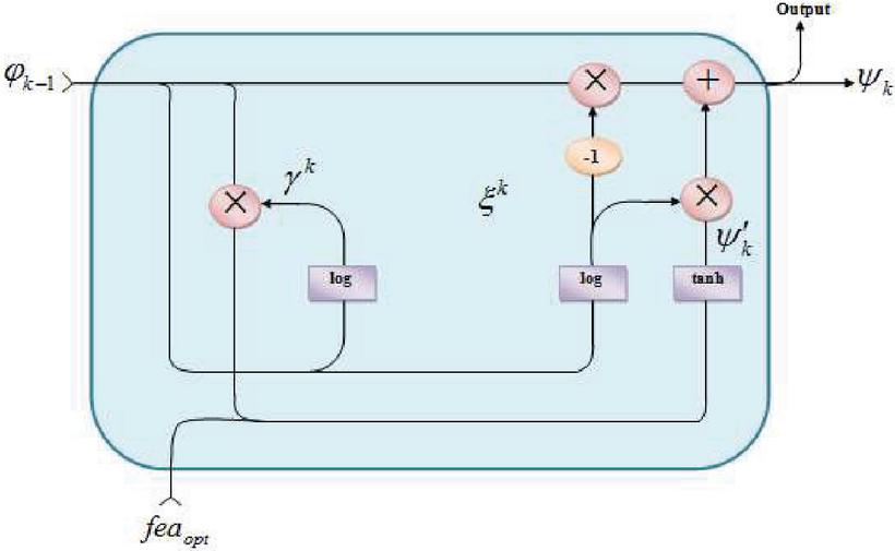
Grounded on the optimal features , the normal panel and the defective panels are classified accurately in this section. The GBLRU method is utilized for classification in the proposed work. A variant of the LSTM design that employs gating mechanisms to allow the model to learn when to update the hidden state and when to forget about the previous hidden state is GRU. GRU is much simpler than LSTM where it merges the input and forget gate into a single gate and discards the cell state. Hence, the two gates that are reset and updated are contained in the GRU. Gradient vanishing and exploding issues are present in the conventional Gated Recurrent Unit (GRU). Also, while utilizing the tanh or relu activation function, the long sequences cannot be processed by the unit. The logarithmic Softmax (Logmax) activation function is used in the gated recurrent unit to tackle this complication. The misclassification was led by the weight updating in a random manner. To update the weight, Bernoulli’s distribution function was utilized in the proposed work. To classify the normal panel and defective panel, the proposed classifier is utilized. Figure 2 exhibits the architecture of GBLRU.
Figure 2 Architecture of GBLRU algorithm.
At each time, two inputs incorporating the current input and the prior hidden state as vectors were taken by each gate. By executing the element-wise multiplication betwixt the concerned vector and the respective weights for each gate along with the non-linear input transformation, the output of each gate is obtained. Utilizing Bernoulli’s distribution function, the weights are initialized to diminish the training time as well as the misprediction rates. The function is given as,
| (24) |
Where, the probability of success is demonstrated as , and is the weight vector initialized utilizing the distribution function. The two primary gates functioning in GRU with the activation function are as follows,
Reset Gate: The quantity of past information to forget was decided by the reset gate. It is parallel to the amalgamation of input and forget gate present in the LSTM network. By a linear sum betwixt the newly computed state and the prevailing state with the bias parameter, the update gate is computed. It can be articulated as,
| (25) | |
| (26) |
Where, the reset gate determined by the input vector is signified as , the information at the prior moment are the fixed-sized parameters like weights and bias, and is the Logarithmic Softmax (Logmax) activation function.
Update Gate: The output gate in the LSTM recurrent unit resembled the update gate that determines the quantity of information as of the prior steps is needed to be retained. The update gate can be computed as,
| (27) | |
| (28) |
Where, is the update gate which was calculated by the newly computed state and prevailing state with the bias parameter.
To pass the relevant information, the reset gate was required by the current memory content whereas, the information for the current unit was holded by the final memory unit along with passes to the network utilizing the update gate. Hence, the memory states are computed as,
| (29) | |
| (30) |
Where, the hyperbolic tangent function was notated as . Using , an update gate represents forgetting the previous hidden state , while representing the information memory contained about the present node . To process the first symbol in the sequence of input, the unit was forced by the reset gate when is off. Thus, it allows eliminating the priory computed state .
The network’s output resulted in two classes namely the normal panel and defected panel , once the learning process is accomplished by analyzing the input features.
3.6 Hotspot Detection
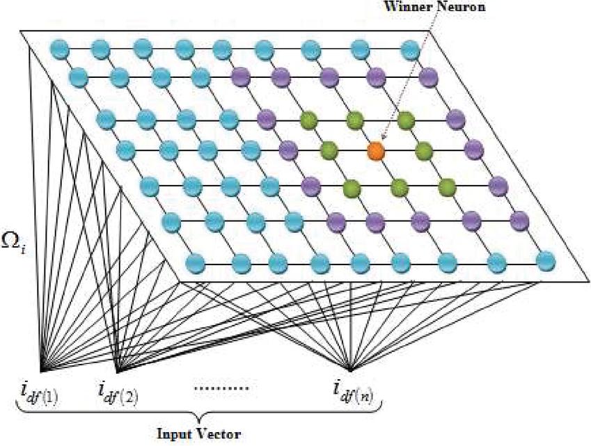
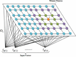
To segment the SP’s hotspot, the HSOM is utilized after the defective panel’s classification. For clustering, Self-Organizing Map (SOM) is used. To map multidimensional data onto lower-dimensional, mapping techniques are utilized. Two significant layers namely the input layer and the competitive layer are comprised in the SOM. The competitive layer is also known as the feature map. Mutually competitive relationships were found in the competitive layer neurons that may compete to become the best-matching unit (BMU). The input samples’ current classification pattern was represented by the BMU. However, a common distance measure that does not scale invariant is the Euclidean distance, which is utilized for data clustering. Grounded on the feature’s units, the distances calculated might be skewed which was meant by scale invariant. Before utilizing this distance measure, one needs to typically normalize the data. Rather than Euclidean distance, the need for normalization was averted by the Haversine distance, which was utilized here. Figure 3 exhibits the SOM structure.
Figure 3 Structure of SOM.
Step 1: The mapping step commences with initializing the weight vector. The weight of size is initialized and is the number of clusters. To identify which weight represents that sample in a better way, a sample vector is chosen randomly along with searching the map of weight vectors. The input vector is initialized as,
| (31) |
Step 2: To identify the BMU, the distance betwixt the randomly chosen vector and the node’s weight vector was computed to track the node with the petite distance.
| (32) | ||
| (33) | ||
| (34) |
Where, the latitude of two points was denoted as , the longitudes of two points were signified as , denotes the Haversine distance.
Step 3: The neuron with minimal distance which is identical to the input vector is declared as BMU in correspondence to the input vector. The BMU’s weight vector is updated as,
| (35) |
Where, the learning rate function is illustrated as . The proposed HSOM algorithm’s pseudocode was exhibited in Algorithm 2.
Algorithm 2: Pseudo code of HSOM algorithm
| Input: Defected panels |
| Output: Segmented Hotspot |
| Begin |
| Initialize input vector, neurons, weights, maximum number of iterations |
| While |
| Select randomly |
| Find winning neuron for the sample input |
| Compute Haversine distance |
| If |
| { |
| Find BMU best matches the input |
| Update weights of BMU |
| Else |
| Select the next input sample |
| } |
| End if |
| Reduce learning rate |
| Return segmented hotspot of PV panels |
| End |
As per the above algorithm, all input samples have been learned. Thus, the HSOM network converges and returns the solar panel’s segmented hotspot.
4 Result and Discussion
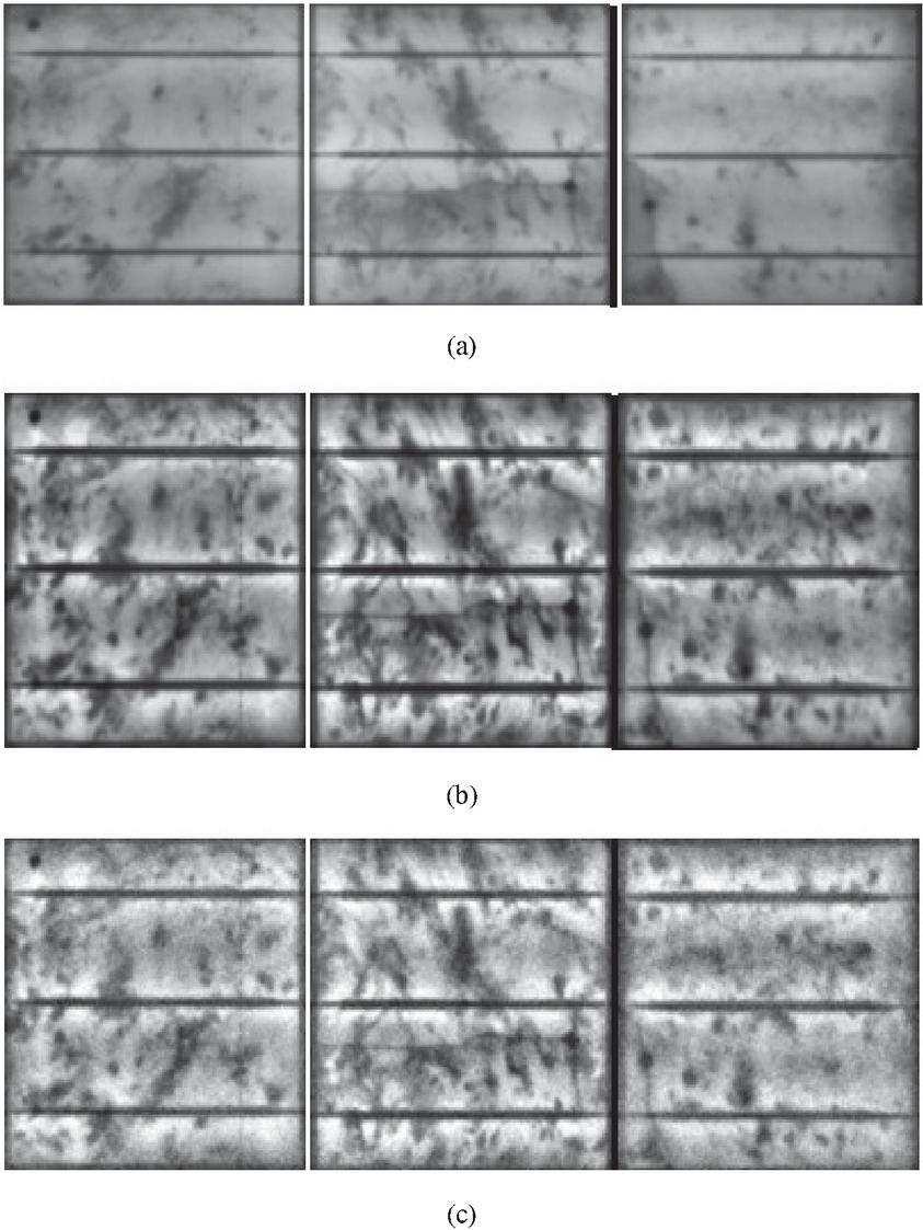
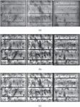
By doing several experiments on MATLAB (version R2020a), the proposed hotspot detection system’s performance was evaluated here. The images captured during the PV plants’ inspection are contained in the PV thermal image dataset, which was utilized for the performance analysis in this work. Figure 4 illustrates the sample images of the datasets and the image’s further process.
The sample images utilized for the performance analysis was shown in Figure 4. The dataset’s input image is exhibited in Figure 3(a). The enhanced image after color conversion utilizing the MHB algorithm is illustrated in Figure 4(b). Also, the detected panels utilizing the Log Inverse Bilateral Edge Detector (LIBED) were illustrated in Figure 4(c).
4.1 Performance Analysis
Utilizing the performance metrics like Sensitivity, Specificity, Accuracy, Precision, Recall, F-measure, Negative Predictive Value (NPV), False Positive Rate (FPR), False Negative Rate (FNR), Matthews Correlation Coefficient (MCC), False Discovery Rate (FDR), and False Rejection Rate (FRR), etc, the proposed GBLRU’s performance was analogized with the prevailing Gated Recurrent Unit (GRU), Deep Neural Network (DNN), and Recurrent Neural Network (RNN) in this section.
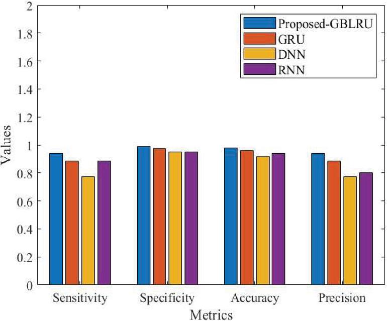
The proposed GBLRU and prevailing techniques’ evaluated values are exhibited in Table 1. When analogized to the prevailing GRU method, the proposed model elevated its sensitivity score, specificity, accuracy score, and precision value by 5.61%, 1.27%, 2.07%, and 5.61%. An accuracy value of 0.939583 was proffered by the prevailing RNN which was found to be 5.61% lower than the proposed classifier. Likewise, DNN also attains less accuracy and shows lower performance for all performance metrics compared to the GBLRU, which is contrary to the other prevailing schemes. Regarding defective panel detection and classification, it is evident as of the attained analysis outcomes that an enhanced performance was illustrated by the proposed methodology. Figure 5 illustrates the above table’s graphical representation.
Figure 4 Sample images of the dataset, (a) input image, (b) Color Corrected image, and (c) edge detected image.
Table 1 Analysis of the performance of the proposed classifier with the existing classifiers based on the quality metrics
| Methods/Metrics | Sensitivity | Specificity | Accuracy | Precision |
| Proposed GBLRU | 0.94382 | 0.987277 | 0.979253 | 0.94382 |
| GRU | 0.88764 | 0.974555 | 0.958506 | 0.88764 |
| DNN | 0.775281 | 0.949109 | 0.917012 | 0.775281 |
| RNN | 0.885057 | 0.951654 | 0.939583 | 0.802083 |
Figure 5 Performance Analysis based on sensitivity, specificity, accuracy, and precision.
Table 2 Evaluates the performance of the proposed and existing classifiers
| Methods/Metrics | Recall | F-measure | NPV |
| Proposed GBLRU | 0.94382 | 0.94382 | 0.987277 |
| GRU | 0.88764 | 0.88764 | 0.974555 |
| DNN | 0.775281 | 0.775281 | 0.949109 |
| RNN | 0.885057 | 0.84153 | 0.973958 |
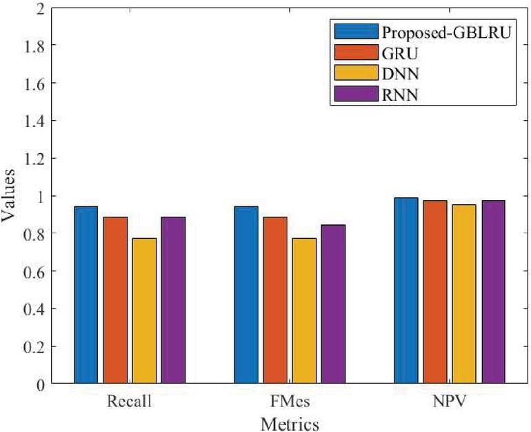
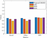
Regarding recall, F-Measure, and NPV metrics, the GBLRU classifier’s performance was analyzed with the GRU, DNN, and RNN classifiers in Table 2. The proposed classifier’s recall and F-Measure value are higher, which is 5.61% more than the prevailing GRU, 16.8% more than DNN, and 5.87% more than RNN methods. Lower results of 0.9745 for GRU, 0.9491 for DNN, and 0.9739 for RNN were obtained by the prevailing models regarding NPV. This table determines that the worst performance was attained by the prevailing DNN algorithm than the prevailing models and the proposed schemes. Better performance than the other prevailing models was attained by the prevailing GRU algorithm but not better than the proposed GBLRU. Therefore, it concludes that when analogized with the prevailing models like GRU, DNN, and RNN, better performance in defective panel classification systems was attained by the proposed GBLRU system. Figure 6 exhibits the pictorial representation of Table 2.
Figure 6 Performance Analysis with Reference to Recall, F-measure, and NPV.
Table 3 Illustrates the Performance of the Proposed and Existing Classifiers with Respect to False Predictions
| Methods/Metrics | FPR | FNR | MCC | FRR |
| Proposed GBLRU | 0.012723 | 0.05618 | 0.931098 | 0.05618 |
| GRU | 0.025445 | 0.11236 | 0.862195 | 0.11236 |
| DNN | 0.050891 | 0.224719 | 0.72439 | 0.224719 |
| RNN | 0.048346 | 0.114943 | 0.805806 | 0.114943 |
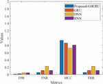
The proposed and existing classifiers’ experiential analysis is exhibited in Table 3. An FPR of 0.012723, an FNR of 0.05618, and an FRR of 0.5618 were achieved by the proposed model. When analogized with the proposed system, the prevailing algorithms comparatively engendered elevated false error rates. The system’s efficacy will be high if the false predictions are lower. Likewise for MCC, the proposed model attains higher outcomes as 0.93109, which is 6.89% higher than the existing GRU. Henceforth, the proposed method attained a higher value for negative predictions and lower error rates for false predictions which exhibited that better performance was exhibited by the proposed scheme by elevating the classification accuracy. Figure 7 illustrated the graphical illustration of the above Table 3.
Figure 7 Performance Analysis regarding FPR, FNR, MCC, and FRR.
4.2 Comparative Analysis
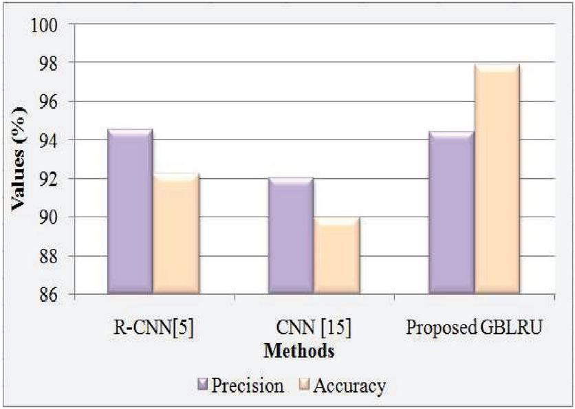
To validate the proposed system’s efficacy, the experiential outcomes obtained for the prevailing models are analogized with the prevailing Region based Convolution Neural network (R-CNN [5]), and Convolution Neural network (CNN [5]) in this section.
Figure 8 Comparative analysis.
By analogizing the proposed system’s outcomes with the prevailing frameworks, its effectiveness is analyzed in Figure 8. When analogized to the prevailing R-CNN [5], the proposed system improved its accuracy by 5.67%. In contrast to the CNN [15] model, an elevated outcome with an increase of 2.38% is obtained regarding precision. Hence, the analysis concludes that the defective modules were differentiated from the normal modules by the various steps proposed in this algorithm.
5 Conclusion
A novel algorithm for SP hotspot detection has been proposed in the work. Several operations like Thermal Image database collection, Colour correction, Panel Detection, Feature Extraction, Feature Selection, Classification, and Hotspot detection are included in the proposed framework. Utilizing the HSOM technique, the proposed framework effectively categorizes the defective panels and precisely segments the detected hotspot. To validate the proposed algorithm’s effectiveness, the experiential analysis is then carried out, in which the proposed GBLRU technique is compared and performance-analyzed regarding a few performance metrics. The final result shows that 97.92% of accuracy was attained by the proposed model. As a result, the proposed methodology performs better than the current state-of-the-art methods, produces more encouraging findings, and continues to be more trustworthy and sturdy. To elevate the FD system, this work can be extended in the future to particular PV defects with some advanced techniques.
References
Afifah, A. N. N., Indrabayu, Suyuti, A., and Syafaruddin. (2020). Hotspot Detection in Photovoltaic Module using Otsu Thresholding Method. 2020 IEEE International Conference on Communication, Networks and Satellite, Comnetsat 2020 – Proceedings, 408–412. https://doi.org/10.1109/Comnetsat50391.2020.9328987.
Akram, M. W., Li, G., Jin, Y., Chen, X., Zhu, C., and Ahmad, A. (2020). Automatic detection of photovoltaic module defects in infrared images with isolated and develop-model transfer deep learning. Solar Energy, 198, 175–186. https://doi.org/10.1016/j.solener.2020.01.055.
Ali, M. U., Saleem, S., Masood, H., Kallu, K. D., Masud, M., Alvi, M. J., and Zafar, A. (2022). Early hotspot detection in photovoltaic modules using color image descriptors: An infrared thermography study. International Journal of Energy Research, 46(2), 774–785. https://doi.org/10.1002/er.7201.
Ali, M. U., Khan, H. F., Masud, M., Kallu, K. D., and Zafar, A. (2020). A machine learning framework to identify the hotspot in photovoltaic module using infrared thermography. Solar Energy, 208, 643–651. https://doi.org/10.1016/j.solener.2020.08.027.
Balasubramani, G., Thangavelu, V., Chinnusamy, M., Subramaniam, U., Padmanaban, S., and Mihet-Popa, L. (2020). Infrared thermography based defects testing of solar photovoltaic panel with fuzzy rule-based evaluation. Energies, 16(3), 1–14. https://doi.org/10.3390/en13061343.
Charfi, W., Chaabane, M., Mhiri, H., and Bournot, P. (2018). Performance evaluation of a solar photovoltaic system. Energy Reports, 4, 400–406. https://doi.org/10.1016/j.egyr.2018.06.004.
Chen, J., Li, Y., and Ling, Q. (2020). Hot-Spot Detection for Thermographic Images of Solar Panels. Proceedings of the 32nd Chinese Control and Decision Conference, CCDC 2020, 4651–4655. https://doi.org/10.1109/CCDC49329.2020.9164255.
Diaz, J. J. V., Vlaminck, M., Lefkaditis, D., Vargas, S. A. O., and Luong, H. (2020). Solar panel detection within complex backgrounds using thermal images acquired by UAVs. Sensors, 20(21), 1–16. https://doi.org/10.3390/s20216219.
Et-Taleby, A., Boussetta, M., and Benslimane, M. (2020). Faults detection for photovoltaic field based on k-means, elbow, and average silhouette techniques through the segmentation of a thermal image. International Journal of Photoenergy, 2020, 1–7. https://doi.org/10.1155/2020/6617597.
Fernandez, A., Usamentiaga, R., de Arquer, P., Fernández, M. A., Fernandez, D., Carús, J. L., and Fernández, M. (2020). Robust detection, classification and localization of defects in large photovoltaic plants based on unmanned aerial vehicles and infrared thermography. Applied Sciences, 10(17), 1–18. https://doi.org/10.3390/app10175948.
Fonseca Alves, R. H., Deus Junior, G. A. de, Marra, E. G., and Lemos, R. P. (2021). Automatic fault classification in photovoltaic modules using convolutional neural networks. Renewable Energy, 179, 502–516. https://doi.org/10.1016/j.renene.2021.07.070.
Henry, C., Poudel, S., Lee, S. W., and Jeong, H. (2020). Automatic detection system of deteriorated PV modules using drone with thermal camera. Applied Sciences, 10(11), 1–16. https://doi.org/10.3390/app10113802.
Hernandez-Callejo, L., Gallardo-Saavedra, S., and Alonso-Gómez, V. (2019). A review of photovoltaic systems: Design, operation and maintenance. Solar Energy, 188, 426–440. https://doi.org/10.1016/j.solener.2019.06.017.
Huerta Herraiz, A., Pliego Marugan, A., and Garcia Marquez, F. P. (2020). Photovoltaic plant condition monitoring using thermal images analysis by convolutional neural network-based structure. Renewable Energy, 153, 334–348. https://doi.org/10.1016/j.renene.2020.01.148.
Jeong, H., Kwon, G. R. and Lee, S. W. (2020). Deterioration diagnosis of solar module using thermal and visible image processing. Energies, 13, 1–14. https://doi.org/10.3390/en13112856.
Kenu E. Sarah. (2020). A Review of Solar Photovoltaic Technologies. International Journal of Engineering Research And, 9(7), 741–749. https://doi.org/10.17577/ijertv9is070244.
Lee, S. W., An, K. E., Jeon, B. D., Cho, K. Y., Lee, S. J., and Seo, D. (2018). Detecting faulty solar panels based on thermal image processing. IEEE International Conference on Consumer Electronics, 1–2. https://doi.org/10.1109/ICCE.2018.8326228.
Mellit, A., Tina, G. M., and Kalogirou, S. A. (2018). Fault detection and diagnosis methods for photovoltaic systems: A review. Renewable and Sustainable Energy Reviews, 91, 1–17. https://doi.org/10.1016/j.rser.2018.03.062.
Menendez, O., Guamán, R., Pérez, M., and Cheein, F. A. (2018). Photovoltaic modules diagnosis using artificial vision techniques for artifact minimization. Energies, 11(7), 1–23. https://doi.org/10.3390/en11071688.
Niazi, K. A. K., Akhtar, W., Khan, H. A., Yang, Y., and Athar, S. (2019). Hotspot diagnosis for solar photovoltaic modules using a Naive Bayes classifier. Solar Energy, 190, 34–43. https://doi.org/10.1016/j.solener.2019.07.063.
Salamanca, S., Merchan, P., and Garcia, I. (2017). On the detection of solar panels by image processing techniques. 25th Mediterranean Conference on Control and Automation, 478–483. https://doi.org/10.1109/MED.2017.7984163.
Salazar, A. M., and Macabebe, E. Q. B. (2016). Hotspots Detection in Photovoltaic Modules Using Infrared Thermography. MATEC Web of Conferences, 70, 1–5. https://doi.org/10.1051/matecconf/20167010015.
Pierdicca, R., Paolanti, M., Felicetti, A., Piccinini, F., and Zingaretti, P. (2020). Automatic faults detection of photovoltaic farms: Solair, a deep learning-based system for thermal images. Energies, 13(24), 1–17. https://doi.org/10.3390/en13246496.
Wang, Q., Paynabar, K., and Pacella, M. (2021). Online automatic anomaly detection for photovoltaic systems using thermography imaging and low rank matrix decomposition. Journal of Quality Technology, 1–14. https://doi.org/10.1080/00224065.2021.1948372.
Wlodarczak, P. (2019). Learning Techniques. Machine Learning and Its Applications, 14, 149–160. https://doi.org/10.1201/9780429448782-9.
Biographies

P. Pradeep Kumar received the B.Tech Degree in Electrical & Electronics Engineering from G.Pullaiah College of Engineering and Technology in 2012, M.Tech Degree from JNTU Anantapur in 2015. Currently, Pursuing Ph.D Degree from JNTU ANANTAPUR Under the guidance of Dr. M. Rama Prasad Reddy, Professor fron G.Pullaiah College of Engineering and Technology, Kurnool, A.P. His areas of interests are in Power Electronic control of Drives and Renewable Energy Sources.

M. Rama Prasad Reddy received the B.E Degree in Electrical & Electronics Engineering from Karnataka University of Dharwad in 1999, M.Tech Degree from JNTU Kakinada in 2007 and Ph.D Degree from JNTU Hyderabad in 2015. Currently, working as Professor in G.Pullaiah College of Engineering and Technology, Kurnool, A.P. He is published more than 50 publications in various reputed Journals and Conferences. His areas of interests are in Power Electronic control of Drives and Renewable Energy Sources.
Distributed Generation & Alternative Energy Journal, Vol. 39_1, 165–194.
doi: 10.13052/dgaej2156-3306.3917
© 2023 River Publishers
