A Novel Opposition-Based Border Collie Optimization Approach for Fault Detection in Solar Photovoltaic Array
Sowthily Chandrasekharan, Senthilkumar Subramaniam*, Malakonda Reddy Bhoreddy and Veeramani Veerakgoundar
Department of Electrical and Electronics Engineering, National Institute of Technology, Tiruchirappalli 620 015, India
E-mail: sowthilyc@gmail.com; skumar@nitt.edu; kondareddy232@gmail.com; vveeramani86@gmail.com
*Corresponding Author
Received 24 January 2022; Accepted 12 July 2022; Publication 27 February 2023
Abstract
Solar photovoltaic systems installed in outdoor environments are susceptible to faults and partial shading, which leads to reduction in the production of maximum power. The conventional protection units are unable to detect the types of faults due to non-linear characteristics and they result in fire hazards and reduced system efficiency. In this paper, a fault detection method based on Multiclass Support Vector Machine (MSVM) is proposed to detect different faults like line-ground (L-G), line-line (L-L), and partial shading. The array voltage, array current and irradiance are used to detect the line-line and partial shading under different irradiation conditions. The novel Opposition-based Border Collie Optimization (OBCO) algorithm is used to improve the accuracy of fault classification by optimizing the hyper-parameters of MSVM. A 1.6 kW, 4 4 solar photovoltaic array is developed, and the fault conditions are experimentally tested to validate the proposed algorithm. The experimental results show that the proposed MSVM-OBCO fault detection algorithm has higher accuracy compared to that of the existing classification algorithms such as -nearest neighbor, Naïve Bayes, Decision Tree and Random Forest.
Keywords: Fault detection, solar photovoltaic system, line-line fault, multiclass SVM, one vs all classifier, machine learning, opposition-based learning, border collie optimization.
1 Introduction
In recent years, the utilization of solar energy is receiving more attention because of the huge energy crisis. Solar energy is available in abundance. It is pollution-free, environment friendly, and requires low maintenance. During the last few decades, there is an exponential rise in the installation capacity of Photovoltaic (PV) Systems [1]. A solar PV system is comprised of panels connected in both series and parallel. The cables used for connecting the panels may cause Line-Line faults (L-L faults) and Line-Ground faults (L-G faults). The power efficiency of the panels may get reduced because of ageing, shadow (Partial Shading), and hotspots in the PV arrays [2]. The proposed paper focuses on L-L faults and Partial Shading. L-L faults are caused by failure in the connection between cables due to animal chewing, ageing of wires and damage in the combiner box. Partial Shading is a mismatch fault, it is temporary in nature. These faults cause energy losses, degradation of panels and fire hazards if not cleared by proper protection devices [3, 4].
The installations of PV systems worldwide follow the protection standards as stated in U.S. National Electric Code (NEC) to use Over-Current Protection Device (OCPD) and Ground Fault Protection Device (GFPD) for detection and clearing of short-circuit faults like L-L and L-G faults respectively. But due to the operation of Maximum Power Point Tracking (MPPT), blocking diodes in the PV system and environmental conditions, conventional OCPD and GFPD often fail to detect LL fault and shading [5]. Hence, the researchers have discussed various protection challenges in solar PV systems and developed a fault detection method for L-L faults. Murtaza et al. proposed a fault-finding algorithm uses the measured incoming and outgoing current data from each string to identify the PV faults. However, this method requires a greater number of sensors, controllers, and additional hardware setups [6]. Rakesh et al. proposed a method based on a simple observation from the Current versus Voltage (I-V) characteristic curve of PV array at Line-Line (L-L) fault. This type of fault is detected using the variable Gamma, which are continuously updated from PV array voltage, current, and irradiation [7]. Chandrasekaran et al. developed a simple analysis for fault detection under different fault conditions, such as line-line (L-L) fault, line-ground (L-G) fault and short-circuit fault with multiple strings, and the values of the current indicator and threshold are predetermined. Based on these values, the fault detection algorithm identifies the fault in the PV array and the PV string, with a reduced number of current sensing devices [8]. Maleki et al. proposed an algorithm based on kurtosis function to discriminate fault condition and partial shading [9]. Hariharan et al. proposed a fault detection algorithm that analyzes the P-V characteristics under partial shading and fault condition. Nevertheless, it is challenging to discriminate temporary faults due to the fault condition and is challenging to evade malfunctioning of the protection units [10].
Artificial Intelligence (AI) plays a main part in the diagnosis of faults. Convolutional Neural Network (CNN) has been used for PV fault detection and classification with three indicators: normalized PV array current, normalized PV voltage, and fill factor. This method has been experimentally tested to detect the PV faults [11]. A combination of continuous wave transforms and an existing pre-trained CNN- AlexNet has been used to detect and classify the PV faults. This method uses the I-V characteristics of a PV system to detect and classify faults, including arc, line-to-line, open circuit, and partial shading faults [12]. However, in CNN, the number of layers increases with the increase in the size of the PV array. In addition, over-fitting and under-fitting issues are the major disadvantages of the neural network, owing to the uncertain count of the hidden layer nodes. The other drawbacks include poor accuracy and inability to predict exact faults in the solar PV array.
Machine learning (ML) classifiers [13] are widespread in which the model is trained with historic data to predict and classify different faults. Badr et al. aims an optimal Machine Learning (ML) structure of automatic fault detection and diagnosis algorithm for common PV array faults, namely, permanent faults (Arc Fault, Line-to-Line, Maximum Power Point Tracking unit failure, and Open-Circuit faults), and temporary faults (Shading) under a wide range of climate datasets, fault impedances, and shading scenarios. Bayesian Optimization is adopted to assign the optimal hyperparameters to the fault classifiers [14]. Decision Tree (DT) has been used to detect line-to-line, open circuit, and partial shading faults. The input parameters were ambient temperature, solar irradiance, and the ratio of the calculated power to the measured power. The model-specific type of DT detected and classified string, short circuit, and line-to-line faults. However, mismatch faults are not identified exactly as it requires larger training data [15]. Ziane et al. proposed a method to detect and classify the partial shading conditions in a grid tied PV system using Random Forest algorithm [16]. Solar fault detection methods based on Support Vector Machine (SVM) are becoming popular to diagnose the short circuit faults. Wang et al. used an optimized SVM with grid search and k-fold cross-validation to detect short-circuit, open-circuit, and shading faults in PV arrays. The input parameters of the SVM were I-V characteristics curves, short-circuit current, open-circuit voltage, maximum power-current, and maximum power-voltage [17]. Harrou et al. proposed an unsupervised learning procedure to detect the solar PV faults and shading using one-class Support Vector Machine [18]. Yi et al. offered an advanced approach using two stage Support Vector Machine for identifying short circuit faults in PV arrays. A multi-resolution signal decomposition process is used to extract the significant features [19].
Jufri et al. presents the development of a PV fault detection system by combining regression and Support Vector Machine models. The regression model is used to estimate the expected power generation under the respective solar irradiance, which is used as the input for the SVM model [20]. Esksndari et al. proposed a method based on the SVM and Genetic algorithm to classify the PV faults. The features are extracted by analyzing the Current-Voltage (I-V) characteristics under various L-L faults and normal operation. Genetic Algorithm (GA) is used for parameter optimization of the kernel functions used in the Support Vector Machine classifier [21]. However, the existing techniques may need a complex and long-term training procedure that can influence their efficiency and these methods require a larger dataset for the learning process. Another drawback of these SVM based methods is low accuracy in detecting the L-L faults.
To overcome the above limitations, this paper proposes a fault detection algorithm based on Multiclass Support Vector Machine (MSVM) is developed to detect the faults in solar PV arrays. A novel Opposition based Border Collie Optimization (OBCO) algorithm is used to optimize the hyper-parameters in MSVM and improves the accuracy of fault classification. The rest of this paper has the following organization. Section 2 presents the typical faults in solar photovoltaic array. Section 3 explains the Methodology for the proposed fault detection. Section 4 presents the Experimental setup and verification, and the Section 5 gives the Performance analysis using MSVM based OBCO. The main conclusions are summarized in Section 6.
2 Typical Faults in Solar Photovoltaic Array
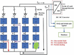
The L-G fault occurs due to an unintentional current path of low impedance between one of the current-carrying conductors and the ground. It is caused due to damage in the insulation of the cables during installation or because of chewing cables by rodents, accidental short-circuit inside the DC junction box at the time of maintenance, corrosion, ageing or mechanical damage. If the L-G fault remains unobserved, it may lead to fire. The L-L fault happens when an accidental low impedance current flow comes between two points of the same or nearby strings at different potentials in a PV system. During L-L fault, it is observed that the current flow in the faulty string is reversed, and its magnitude depends on the potential difference across the two fault points in the PV system. Partial shading occurs due to mismatches in the PV modules because of shading from buildings, chimneys, light posts, clouds, trees, dirt, snow, and other light-blocking objects/obstacles. Generally, partial shading is classified as a temporary fault. To analyze the proposed method, a 4 4 array connected to the grid system is considered as shown in Figure 1.
Figure 1 Typical faults in Solar PV array.
3 Proposed Fault Detection Method
3.1 Support Vector Machine
The main motive behind the usage of SVM is to obtain an accurate classification of various instances without involving much computational expenditure. SVM is universally employed to detect and classify faults from normal condition. It deals with linear and nonlinear classification problems with binary classification and regression. The hyperplane is structured as a decision boundary for classification between two data classes. The data-points near the hyperplane, which imparts construction of the hyperplane is considered as Support Vector Machine (SVM) [22]. The optimized hyperplane can be expressed as
| (1) |
where is the weight vector, is the input vector and represent the bias. The binary classification problem has two class labels, and so it is easy to train the data and predict the outputs. Multi-class classification models are preferred because the solar fault diagnosis contains more number of class labels to analyze the fault condition.
3.2 Multiclass SVM
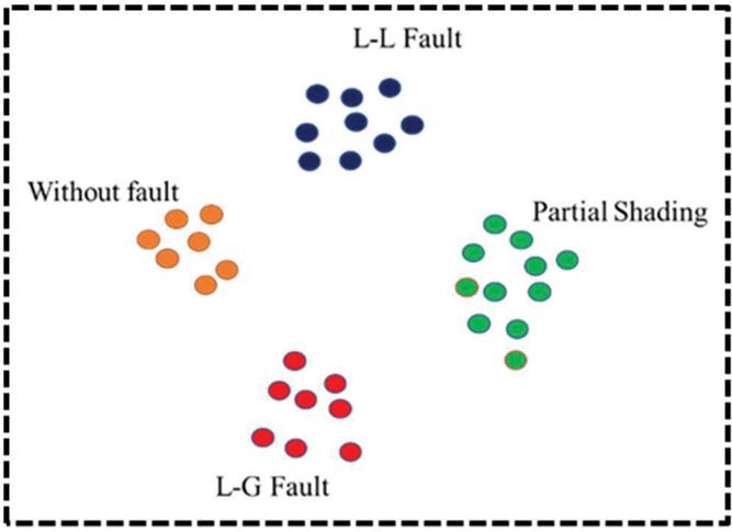
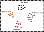
Multiclass classification is a technique that categorizes the test data into multiple class labels [23]. A Multiclass SVM (MSVM) algorithm is used to categorize the solar PV array faults as given in Figure 2.
Figure 2 Multiclass SVM classification.
The four different solar faults considered are L-L fault, L-G fault, temporary fault, and no-fault condition. The dataset is the input given to the MSVM, and the features are extracted from the input dataset. There are two different techniques available to classify faults for multiclass classification problems. They are One Versus One (OVO) and One Versus All (OVA). Among these, the One vs All classifier is used in this paper to classify the solar faults due to its greater accuracy level. The One vs All classifier can split a multi-class classification dataset into multiple binary classification problem.
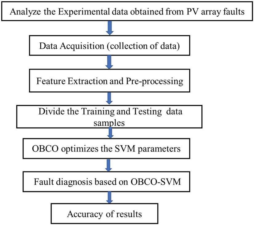
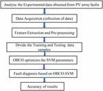
The OVA method has a “” binary classification model where “” is the number of classes. The proposed fault classification is done for different operating conditions like normal condition (no-fault) (class label: A), L-G fault (class label: B), L-L fault (class label: C), and partial shading (class label: D). Here, we must create four classifiers with four classes in the dataset. Hence, the One vs All classifier is divided into four binary classification problems. The flowchart of the proposed model is shown in Figure 3.
Figure 3 Flowchart for the MSVM based fault detection algorithm.
3.3 Fault Data Collection
The maximum power of 1.6 kW for the PV array under Standard Test Conditions (STC – 1000 W/m and temperature of 25C) is considered for experimentation. The key parameters of the used thin-film PV module under STC are as follows: Maximum power W, Open-circuit voltage V, Maximum power voltage V, Short-circuit current A, and Maximum power current A. A DC-DC boost converter is used to extract the maximum power under different environmental conditions.
A 4 4 small-scale grid-connected PV array is used for experimentation to collect the fault data parameters. The Keysight Agilent Acquisition unit is used to collect the array current, array voltage and irradiance from the PV array. To evaluate the faults, different fault conditions are experimented under different climatic conditions with normal and faulty conditions.
3.4 Feature Extraction
Various types of faults are generated on the PV array and the quantities such as array voltage, array current and irradiance are recorded along with the timestamp. The dataset is recorded in a csv file and the class labels are created for further processing of data. After receiving the data, the dataset is studied to get an idea of the behavior of various parameters with respect to time. The analysis of the dataset gives an understanding between faulted conditions and normal conditions.
The proposed fault detection algorithm uses the array voltage (V), array current (I) and irradiance (G) datasets recorded from Data Acquisition Unit (DAQ) as the input to the Personal Computer (PC). With the help of the primary inputs, two features namely impedance and gamma are extracted to identify the faults. To differentiate the partial shading and L-L faults and to improve the efficiency the parameter Gamma is introduced. The variation in impedance when fault occurs will be reflected in array current over time as well. Moreover, the fault current magnitude is higher on the occurrence of fault. The presence of fault in a PV system will inject extra impedance that causes mismatch and heating losses.
3.4.1 Feature I
Gamma is the ratio of instantaneous irradiance to the product of instantaneous array voltage and the individual string current expressed in (2)
| (2) |
where G is the instantaneous irradiance, is the PV array voltage and is the PV array current.
3.4.2 Feature II
The impedance is the ratio of array voltage and string current which is expressed in (3)
| (3) |
where is the PV array voltage and is the PV array current. The feature analysis along with the primary inputs is taken as the input to the Multiclass SVM.
3.5 Training and Testing Data
The experimental data from the solar PV array is collected and recorded to detect and identify the faults. It should be noted that the training dataset contains 915 instances, the testing dataset contains 262 instances, and the validation dataset contains 131 instances. Instances are the readings obtained from the real time experimentation. Hence, the total number of instances available in the dataset used for experimentation is 1308 instances. From the acquired data, 70% of the total fault data is used for training, and 30% of the fault data is used for testing and validation. The dataset is labelled into four classes based on the faults.
3.6 Opposition-based Border Collie Optimization (OBCO)
The main objective of optimization in the proposed technique is to tune the hyper-parameters (i.e. kernels) of the machine learning classifier to increase the detection rate and the classification accuracy. The candidate solution finding process of Border Collie Optimization (BCO) algorithm is incorporated with opposition-based learning in the proposed model. That is, when finding a solution to a defined problem, simultaneously including its opposed solution might bring more ways for determining a candidate solution that is nearer to the global optimum. During optimization, the opposite candidate solution is initialized as depicted in opposition-based learning [24]. Then the hyper-parameters are tuned through the BCO algorithm mathematically modelled in [25].
BCO is a recent bio-inspired algorithm motivated from the herding nature of the Border Collie dogs. The sheep herding behavior of the Border Collie dogs and their capability to make a judgement and provide adaptive conclusions are mimicked to create the BCO algorithm. In OBCO algorithm, a population of three dogs and sheep are taken into consideration. In real-world, one dog is enough to control the herd. Though the search space is large for numerous optimization problems, three dogs are considered during modelling. The position of dogs and sheep are initialized with random variables.
The algorithm is stimulated from the scenario that the sheep go out for grazing across diverse locations and the dogs are allowed to instruct them back towards the farm. The dogs follow a different tactic for sheep herding mainly including the three processes.
3.6.1 Gathering
In gathering the sheep are controlled by the dogs on both directions and front. The dogs try to gather the sheep and guide them to reach the farm. The sheep going closer to the first dog might follow the path of the first dog, forming a group called gathering. The gathered sheep are selected according to their fitness score is given by
| (4) |
where denotes the fitness of best individual, the second and third best fitness (i.e., and ) are chosen as left-side and right-side dogs. represents the fitness score of the sheep. The positive fitness score depicts that the sheep is closer to the first dog. In such cases, Equation (5) is used to update the velocity of the sheep
| (5) |
Here, defines the velocity of sheep to be gathered at time . It is influenced by and that signifies the velocity and acceleration of the first dog at time and respectively. mention the present position of the gathered sheep.
3.6.2 Stalking
In stalking the dogs adopt to control the sheep. The dogs hang the head down, put the hind legs high and place the tails in the land. The dogs stalk the sheep that comes closer to the left-side and right-side dogs to retain them on the right path. The fitness score of these sheep is observed to be negative. The velocity of left-side and right-side dogs makes a great impact on the velocity of these stalked sheep. The equations for the velocity updation of the stalked sheep are presented below.
| (6) | ||
| (7) | ||
| (8) |
Where and velocity of the right and left dogs, is the velocity of the stalked sheep.
3.6.3 Eyeing
In Eyeing the eye starring process is initiated by the Border collie dogs if the sheep goes astray. The BCO algorithm considers the population of three dogs and sheep for mathematical modeling dogs keep an eye on those sheep that are entirely astray from the right path. This is performed if the fitness score is not enhanced even after several consecutive iterations. The dog with the lowest fitness score is made to walk behind the sheep for eyeing. Thus, they are supposed to undertake retardation as
| (9) | ||
| (10) |
where and represents the retardation velocities of the left-side and right-side dogs respectively at time . In Equation (9), and denotes the acceleration and velocity of the left-side dog, if it possesses the least fitness compared to other dogs. In Equation (10), and denotes the acceleration and velocity of the right-side dog, if it possesses the minimal fitness compared to other dogs. The dog with minimal fitness is chosen as it is supposed to be nearer to the sheep.
3.7 OBCO-MSVM Optimization Algorithm
When OBCO algorithm is applied to optimize the hyper-parameters of MSVM, the kernel function and the associated parameters will be optimized. The optimization process is explained as follows.
Step 1: Consider the population for number of individuals , and estimate the opposite population. Set the maximum number of iterations , and the search dimension, before initializing the velocity, acceleration, and time of each individual (both Border collie dogs 3 and sheep = ).
Step 2: Initialize the support vector machine multi-class parameters (kernel function, standardize).
Step 3: The individual with best fitness is selected as first dog, while the second and third best fitness are termed as left-side dog and right-side dog respectively.
Step 4: Perform the characteristics of Border collie dogs under the MSVM hyper-parameters. Initially, the sheep are gathered using Equation (4). If G is positive, the velocity of sheep is updated using Equation (5). If G is not positive, the sheep are stalked using Equation (8). If the fitness is found to be not improved in successive iterations, then eyeing is performed using Equations (9) and (10).
Step 5: The acceleration and time of each individual is updated after performing the characteristics of Border collie dogs.
Step 6: Perform the cyclic calculation until the maximum iteration is reached. Otherwise, obtain the hyper-parameters of SVM model and diagnosis the faults.
4 Experimental Verification
4.1 Laboratory Setup
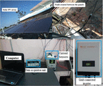
The experimental setup consists of solar PV panels, grid inverter, sensors, and data acquisition (DAQ) unit. The input parameters like array voltage, array current and irradiance are acquired from the solar panel with DAQ unit. The recorded dataset from the data acquisition unit is collected using the USB drive and the array voltage, array current and irradiance is plotted as the waveforms through the Personal Computer (PC). The sampling time of the recorded data is two samples in one second. Data pre-processing is done with the data collected from the experimental setup. The gamma and impedance features are computed and then the kernel parameters are selected. The training and testing processes are performed using the extracted features.
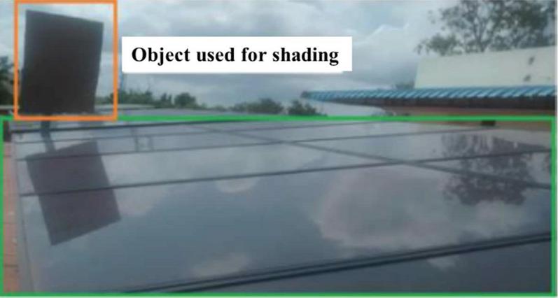
Figure 4 shows the hardware setup and the Line-line fault created between panels. The 4 4 PV array with the thin-film modules is used to collect the dataset with the hardware setup. A switch is used to creates faults between panels. LV 25p LEM voltage sensors and LA 55 LEM current sensors are used to measure the current and voltage readings. The Perturb and Observe MPPT algorithm is incorporated in the Industrial Standard Omnisol Inverter. The Keysight data acquisition unit is used to record the data from the modules. Shading is created by using cardboard, where the shadow falling on the solar PV panel can be seen in Figure 5. To validate the proposed MSVM algorithm, different conditions such as short circuit faults and temporary fault are considered.
Figure 4 Hardware setup.
Figure 5 Partially shaded PV modules.
4.2 Experimental Waveforms
The waveforms are plotted with the readings obtained from the DAQ unit using USB drive. These are the experimental waveforms to show that the faulty conditions are considered in the proposed algorithm. These waveforms are only the input data to the PC. The datasets are taken as the input to the PC for the accurate classification of faults under proposed algorithm.
4.2.1 No-fault condition
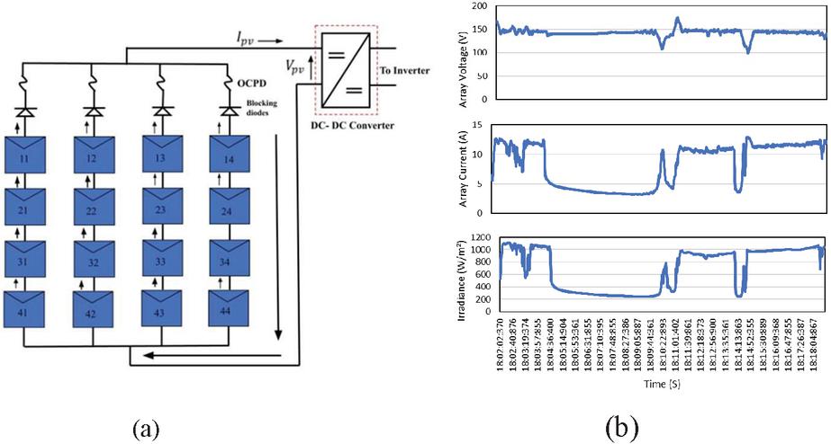
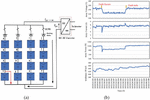
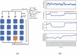
Figure 6(a) shows the No fault condition in PV array and Figure 6(b) illustrates the experimental dataset waveform under no-fault conditions. The datasets obtained from the Agilent DAQ unit without any fault condition is plotted as the waveform. Due to heavy clouds, there is a huge variation in the irradiance. The array current and array voltage gets changed based on the incident irradiance. The maximum power generated from the solar PV array gets varied according to the variation in the irradiance.
Figure 6 (a) No-fault in PV array (b) Waveform plotted for No fault condition.
4.2.2 Line-Line fault (one module mismatch)
An L-G fault is generated in string 1 at panel 41 as shown in Figure 7(a) and 7(b) depicts the experimental dataset waveforms in the L-G fault condition. The datasets obtained from the Agilent DAQ unit with L-G fault condition is Plotted as the waveform. The waveforms are plotted with the datasets obtained from the USB drive. From Figure 7(b) it is depicted that if the fault occurs the array voltage decreases from 146 V to 126 V and the array current remains the same. The maximum power gets reduced because of the reduction in the array voltage.
Figure 7 (a) L-G fault in PV array (b) Waveform plotted for L-G fault condition.
4.2.3 Line-Line fault (two modules mismatched)
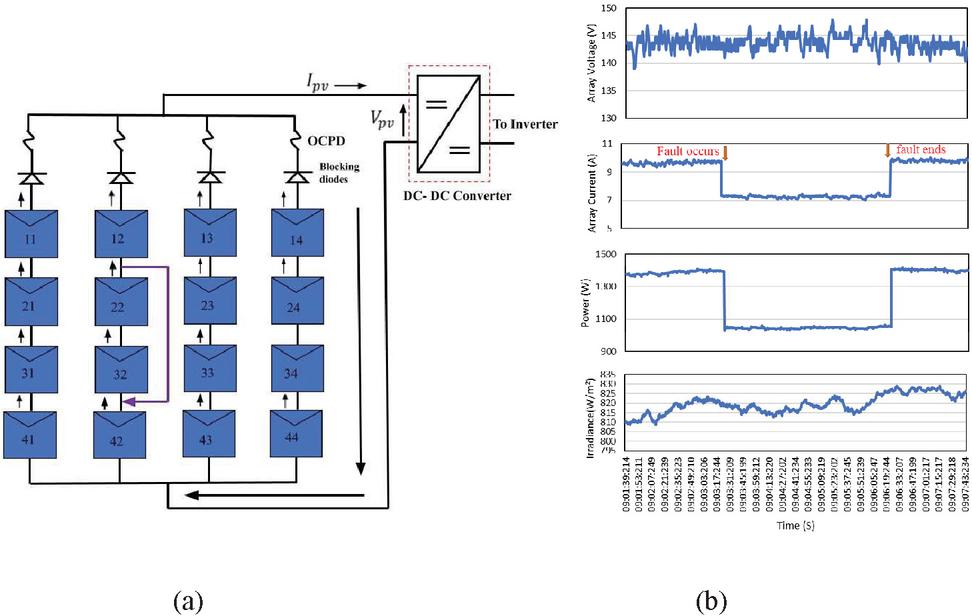
The L-L fault is created in string 2 between panel 12 and panel 42 as shown in Figure 8(a). The experimental dataset outcomes of the L-L fault are shown in Figure 8(b). The datasets obtained from the Agilent DAQ unit with L-L fault condition is Plotted as the waveform. The waveforms are plotted with the datasets obtained from the USB drive. From the experimental results, it is noted that when the fault occurs the array current drops from 9.6 V to 7.1 V. When the L-L fault occurs, string 2 gets open circuited due to the back feed current from the blocking diode.
Figure 8 (a) L-L fault in PV array (b) Waveform Plotted for L-L fault condition.
Figure 9 (a) Shading of the PV array (b) Waveform plotted for shading condition.
4.2.4 Partial shading
The Figure 9(a) shows the shading panel in the PV array. The experimental dataset waveforms under partial shading conditions are shown in Figure 9(b). The panels are partially shaded with the cardboard in string 3. When the shading occurs, the array current gets reduced gradually and maintains the irradiance path. The array voltage remains the same without any change. Hence, the maximum power under temporary fault condition gets reduced.
5 Performance Analysis Based on MSVM-OBCO
The accuracy measures used for evaluation are sensitivity, specificity, precision, false positive rate (FPR) and Root Mean Square error (RMSE). While comparing the accuracy of the Multiclass SVM and other existing classifiers, before hyper-parameter optimization and after hyper-parameter optimization, the accuracy after hyper-parameter optimization is superiorly high for all the classifiers. The proposed Multiclass SVM classifier produces 98.09% accuracy after hyper-parameter optimization and the RMSE is 0.2763 which is relatively less compared to other classifiers. The performance measures are:
5.1 Accuracy
The classification accuracy metric has been introduced to assess the performance of the layers, which is defined based on the confusion matrix. This metric is formulated as
| (11) |
where TP (True Positive) is the case for identification of a data sample correctly, TN (True Negative) is the case for rejection of a data sample correctly, FP (False Positive) represents the case, which is incorrectly identified, and FN (False Negative) is the case which is incorrectly rejected.
5.2 Precision
Precision is calculated as the sum of true positives across all classes divided by the sum of true positives and false positives across all classes.
| (12) |
5.3 Specificity
Specificity is calculated as the true negatives divided by the sum of true negatives and false positives.
| (13) |
5.4 Sensitivity
Sensitivity is calculated by true positives divided by sum of true positive and false negatives.
| (14) |
5.5 FPR
The false positive rate is calculated as
| (15) |
where FP is the number of false positives and TN is the number of true negatives (FP TN being the total number of negatives).
5.6 RMSE
RMSE is the standard deviation of the errors which occur when a prediction is made on a dataset.
The performance of Multiclass SVM based fault classification is determined with and without optimization as shown in Tables 1 and 2 respectively. Furthermore, the performance is compared with different classifiers like Decision Tree (DT) [15], k-Nearest Neighbor (KNN) [26], Naive Bayes (NB) [27] and Random Forest (RF) [16].
Table 1 Parametric comparison before hyper-parameters optimization
| Classifiers | Accuracy | Sensitivity | Specificity | Precision | FPR | F1-Score | RMSE |
| DT | 0.9580 | 0.9466 | 0.9863 | 0.9334 | 0.0137 | 0.9394 | 0.4325 |
| KNN | 0.9542 | 0.9054 | 0.9843 | 0.9386 | 0.0157 | 0.9159 | 0.4144 |
| NB | 0.9389 | 0.9090 | 0.9791 | 0.9242 | 0.0209 | 0.9149 | 0.5990 |
| RF | 0.9695 | 0.9471 | 0.9890 | 0.9592 | 0.0110 | 0.9528 | 0.4004 |
| MSVM | 0.9771 | 0.9593 | 0.9917 | 0.9711 | 0.0083 | 0.9649 | 0.3027 |
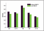
From Table 1, it is observed that the performance of MSVM is better than the existing classifiers. Similarly, the performance of Multiclass SVM with optimization is better than the existing approaches implemented with optimization as seen in Table 2. The Root Mean Square Estimation (RMSE) comparison between different classifier techniques is presented in Figure 10.
Table 2 Parametric comparison after hyper-parameters optimization
| Classifiers | Accuracy | Sensitivity | Specificity | Precision | FPR | F1-Score | RMSE |
| DT | 0.9656 | 0.9584 | 0.9889 | 0.9440 | 0.0111 | 0.9506 | 0.3707 |
| KNN | 0.9618 | 0.9559 | 0.9880 | 0.9373 | 0.0120 | 0.9455 | 0.3808 |
| NB | 0.9466 | 0.9148 | 0.9813 | 0.9385 | 0.0187 | 0.9240 | 0.5386 |
| RF | 0.9733 | 0.9500 | 0.9901 | 0.9681 | 0.0099 | 0.9583 | 0.3549 |
| MSVM | 0.9809 | 0.9683 | 0.9932 | 0.9741 | 0.0068 | 0.9711 | 0.2763 |
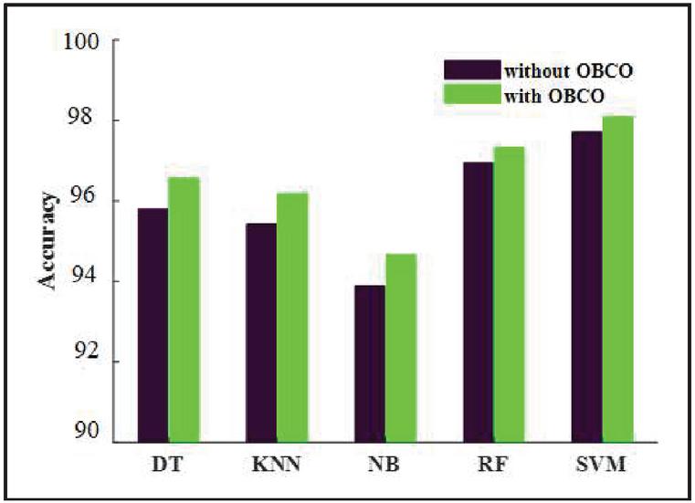
The RMSE is higher if the fault classification is performed without optimization however, it can be reduced if the classification is performed with optimization. The accuracy is higher for the proposed fault detection method compared to other classifier models shown in Figure 11.
Figure 10 RMSE comparison between different classifier models.
Figure 11 Accuracy comparison between different classifier models.
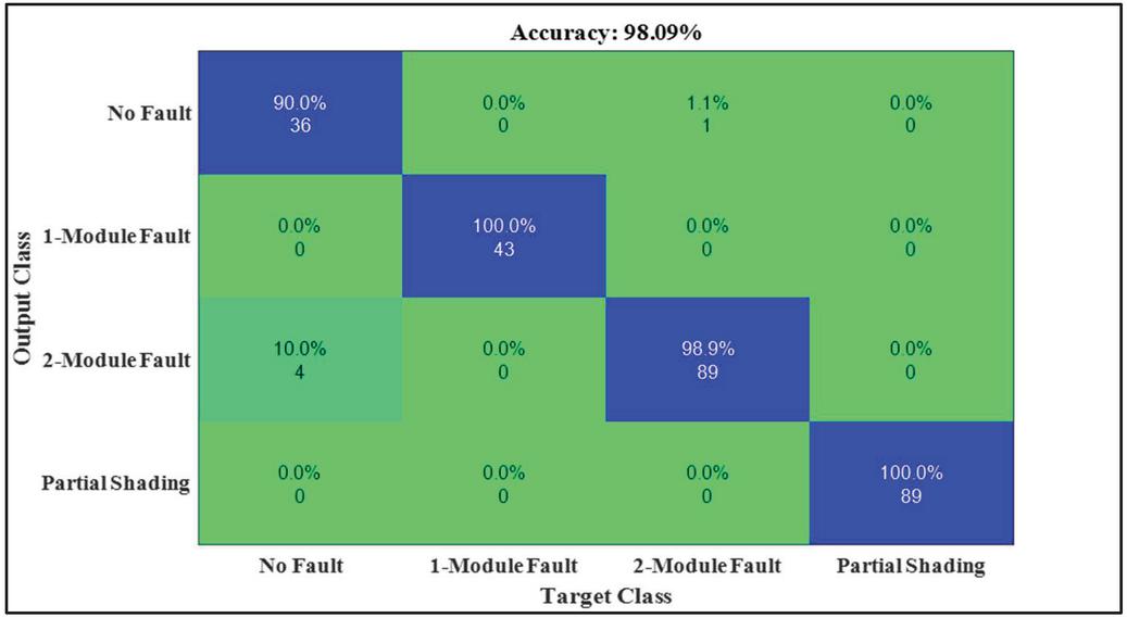
The performance of the fault classification on the testing data is evaluated using confusion matrix, shown in Figure 12. It consists of 4 rows and 4 columns which forms a square matrix. Each main diagonal value represents the number of true positive cases. In Figure 12. the L-L (one module) fault are classified with 100% accuracy and the L-L (two module) fault is classified with 98.9% accuracy. The confusion matrix shows that the OBCO-SVM attains 98.09% accuracy in classifying the faults with the dataset used for testing. It is seen clearly from the confusion matrix that the non-diagonal boxes that give the value zero indicate that in the majority of the fault conditions there is no misclassification.
Figure 12 Confusion matrix for multiclass SVM classifier.
6 Conclusion
The proposed MSVM based fault detection algorithm is validated through the experimental data for a grid connected PV system. The array voltage, array current and irradiance are taken as the input parameters for the proposed algorithm. The two features gamma and impedance are extracted from the input quantities. The learning ability of MSVM is enhanced by optimizing the hyper-parameters of MSVM using the novel OBCO algorithm. The integration of OBCO algorithm to obtain optimal hyper-parameters of the MSVM for classification improved its learning ability. Moreover, the MSVM is observed to be the best fault diagnosis model to classify the four possible scenarios: normal operation, partial shading, L-L fault, and L-G faults. The analysis of fault diagnosis demonstrates that the proposed OBCO-MSVM technique can accurately and efficiently diagnoses the Solar PV faults. Under the same circumstance, the proposed technique has higher fault diagnosis accuracy and recognition efficiency compared to the KNN, RF, NB, and DT classifier algorithms. The confusion matrix shows that the OBCO-SVM attains 98.09% accuracy in classifying the solar PV array faults with the dataset used for testing.
References
[1] Ye Zhao, Jean-François de Palma, Jerry Mosesian, Robert Lyons, Brad Lehman. Line- line fault analysis and protection challenges in solar photovoltaic arrays. IEEE Transactions on Industrial Electronics, Vol. 60, Issue-9, pp. 3784–3795, 2013.
[2] A. Mellit, G. M. Tina, S. A. Kalogirou. Fault detection and diagnosis methods for photovoltaic systems: A review. Renewable and Sustainable Energy Reviews, pp. 1–17, 2018.
[3] M. Mano Raja Paul, R. Mahalakshmi, M. Karuppasamypandiyan, A. Bhuvanesh, R. Jai Ganesh. Classification and Detection of Faults in Grid Connected Photovoltaic System. International Journal of Scientific & Engineering Research, Vol. 7, Issue-4, pp. 149–154, 2016.
[4] D.S. Pillai, R. Natarajan. A comprehensive review on protection challenges and fault diagnosis in PV systems. Renewable and Sustainable Energy Reviews, Vol. 91, pp. 18–40, 2018.
[5] D.S. Pillai, R. Natarajan. A compatibility analysis on NEC, IEC, and UL standards for protection against line–line and line–ground faults in PV arrays. IEEE Journal of Photovoltaics, Vol. 9, Issue-3, pp. 864–871, 2019.
[6] Ali Faisal Murtaza, Mohsin Bilal, Riaz Ahmad, Hadeed Ahmed. A circuit analysis-based fault-finding algorithm for photovoltaic array under LL/LG faults. IEEE Journal of Emerging and Selected Topics in Power Electronics, Vol. 8, Issue-3, pp. 3067–3076, 2019.
[7] Namani Rakesh, Sanchari Banerjee, Senthilkumar Subramaniam, Natarajan Babu. A simplified method for fault detection and identification of mismatch modules and strings in a grid-tied solar photovoltaic system. International Journal of Emerging Electric Power Systems, Vol. 21, Issue-4, pp. 1–16, 2020.
[8] Sowthily Chandrasekharan, Senthil Kumar Subramaniam, Babu Natarajan. Current indicator-based fault detection algorithm for identification of faulty string in solar PV system. IET Renewable Power Generation, Vol. 15, Issue-7, pp. 1596–1611, 2021.
[9] Amir Maleki, Iman Sadeghkhani, Bahador Fani. Statistical sensorless short-circuit fault detection algorithm for photovoltaic arrays. Journal of Renewable and Sustainable Energy, Vol. 11, Issue-5, pp. 1–13, 2019.
[10] R. Hariharan, M. Chakkarapani, G. Saravana Ilango, C. Nagamani. A Method to Detect Photovoltaic Array Faults and Partial Shading in PV Systems. IEEE Journal of Photovoltaics, Vol. 6, Issue-5, pp. 1278–1285, 2016.
[11] Sayed A. Zaki, Honglu Zhu, Mohammed Al Fakih, Ahmed Rabee Sayed, Jianxi Yao. Deep-learning–based method for faults classification of PV system. IET Renewable Power Generation, Vol. 15, Issue-1, pp. 193–205, 2021.
[12] Farkhanda Aziz, Azhar Ul Haq, Shahzor Ahmad, Yousef Mahmoud, Marium Jalal. A Novel Convolutional Neural Network-Based Approach for Fault Classification in Photovoltaic Arrays. IEEE Access, Vol. 8, pp. 41889–41904, 2020.
[13] Ying Yi Hong and Rolando A. Pula. Methods of photovoltaic fault detection and classification: A review. Energy Reports, Vol. 8, pp. 5898–5929, 2022.
[14] Mohamed M. Badr, Mostafa S. Hamad, Ayman S. Abdel Khalik, Ragi A. Hammdy, Shehab Ahmed. Fault Identification of Photovoltaic Array Based on Machine Learning Classifiers. IEEE Access, Vol. 9, pp. 159113–159132, 2021.
[15] Rabah Benkercha, Samir Moulahoum. Fault detection and diagnosis based on C 4.5 Decision tree algorithm for grid connected PV system. Solar energy, Vol. 173, pp. 610–634, 2018.
[16] Abderrezzaq Ziane, R. Dabou, Sahouane Nordine, Mostefaoui Mohammed. Detecting partial shading in grid connected PV station using random forest classifier. International Conference in Artificial Intelligence in Renewable Energetic Systems, Vol. 174, pp. 88–95, 2020.
[17] Junjie Wang, Dedong Gao, Shaokang Zhu, Shan Wang, Haixiong Liu. Fault diagnosis method of photovoltaic array based on support vector machine. Energy Sources, Part A: Recovery, Utilization, and Environmental Effects, pp. 1–16, 2019.
[18] Fouzi Harrou, Dairi Abdelkader, B. Taghezouit, Ying Sun. An unsupervised monitoring procedure for detecting anomalies in photovoltaic systems using a one-class Support Vector Machine. Solar Energy, Vol. 179, pp. 48–58, 2019.
[19] Z. Yi and A. H. Etemadi. Line-to-Line Fault Detection for Photovoltaic Arrays Based on Multiresolution Signal Decomposition and Two-Stage Support Vector Machine. IEEE Transactions on Industrial Electronics, Vol. 64, Issue-11, pp. 8546–8556, 2017.
[20] Fauzan Hanif Jufri, Seongmun Oh, Jaesung Jung. Development of Photovoltaic Abnormal Condition Detection System Using Combined Regression and Support Vector Machine. Energy, Vol. 17, pp. 457–467, 2019.
[21] Aref Esksndari, Jafar Milimonfared, Mohammadreza Aghaei. Autonomous Monitoring of Line-to-Line Faults in Photovoltaic Systems by Feature Selection and Parameter Optimization of Support Vector Machine Using Genetic Algorithm. Applied science, Vol. 10, Issue-16, pp. 1–15, 2020.
[22] Rahul Kumar Mandal, Paresh Kale. Assessment of Different Multiclass SVM Strategies for Fault Classification in a PV System. International Conference on Advances in Energy Research, pp. 747–756, 2021.
[23] A. Mathur and G.M. Foody. Multiclass and binary SVM classification: Implications for training and classification users. IEEE Geoscience and Remote Sensing, Vol. 5, Issue-2, pp. 241–245, 2008.
[24] Moumita Pradhan, Provas Kumar Roy, Tandra Pal. Oppositional based grey wolf optimization algorithm for economic dispatch problem of power system. Ain Shams Engineering Journal, Vol. 9, Issue-4, pp. 2015–2025, 2018.
[25] Dutta T. Bhattacharyya, Dey S. and Platos, J. Border collie optimization. IEEE Access, Vol. 8, pp. 109177–109199, 2020.
[26] Maryam Sabbaghpur Arani and Maryam A. Hejazi. On-line faults detection and classification in PV array using Bayesian and k-nearest neighbor classifier. Journal of Energy Engineering & Management, Vol. 8, pp. 14–25, 2018.
[27] Kamran Ali Khan Niazi, Wajahat Akhtar, Hassan A. Khan, Yongheng Yang, Shahrukh Athar. Hotspot diagnosis for solar photovoltaic modules using a Naive Bayes classifier. Solar Energy, Vol. 190, pp. 34–43, 2019.
Biographies

Sowthily Chandrasekharan received her B.E. Degree in Instrumentation and Control Engineering from Saranathan College of Engineering, Trichy, affiliated to Anna University, Tiruchirappalli, Tamil Nadu, India in the year 2011. She received her M.E. Degree in Control and Instrumentation from J. J. College of Engineering, Trichy, affiliated to Anna University, Chennai, Tamil Nadu, India during the year 2016. She is currently pursuing Ph.D. degree in Electrical and Electronics Engineering at National Institute of Technology, Tiruchirappalli. She worked as an Assistant Professor in the Department of Electronics and Instrumentation Engineering, Mookambagai College of Engineering, Pudukottai, India during 2017–2018. She has also served as a Project Assistant in the DST Funded project during 2018–2020. Her research interests include Renewable Energy System and Optimisation techniques.

Senthilkumar Subramaniam received the B.E. degree in Electrical and Electronics Engineering from Madurai Kamaraj University, Madurai, India, in 1999, the M.Tech. degree in Electrical Drives and Control from Pondicherry University, Puducherry, India, in 2005, and the Ph.D. degree in Electrical Engineering from the National Institute of Technology, Tiruchirappalli, India, in 2013. He has 20 years of teaching experience at various engineering institutions. He is currently working as an Associate Professor with the National Institute of Technology. He has extensively researched on self-excited induction generators for standalone and grid-connected applications. His current research interests include the development of new power converter topologies for renewable energy systems and intelligent transportation systems.

Malakonda Reddy Bhoreddy received the B.Tech degree in Electrical and Electronics Engineering from Narayana Engineering college (Affiliated to JNTU Anantapur), Gudur, S.P.S.R Nellore, Andhra Pradesh, India, in 2011, the M.Tech degree in Power Systems from N.B.K.R Institute of Science & Technology (Affiliated to JNTU Anantapur), Vidyanagar Kota, S.P.S.R Nellore, Andhra Pradesh, India, in 2015 and Ph.D degree in Electrical and Electronics engineering from National Institute of Technology, Tiruchirappalli, Tamil Nadu, India, in 2021. He is currently working as a senior engineer-Electronics with AMIDC (Ati motors), Benglore, Karnataka. His research interest includes power electronics, renewable energy systems and power quality.

Veeramani Veerakgoundar received the B.E degree in Electrical and Electronics Engineering from the National Engineering College, Kovilpatti, India, in 2008, and the M.E. degree in Power Electronics and Drives from Government College of Engineering, Tirunelveli, India, in 2012. He has 5 years of teaching experience at various engineering institutions. He is currently pursuing the Ph.D. degree at the National Institute of Technology, Tiruchirappalli, India. He has been working in the area of power converters for Electric Vehicles applications since 2019.
Distributed Generation & Alternative Energy Journal, Vol. 38_3, 1007–1032.
doi: 10.13052/dgaej2156-3306.38313
© 2023 River Publishers

