Multi-objective Optimal Scheduling Analysis of Power System Based on Improved Particle Swarm Algorithm
Gong Mengting
School of Management, Xi’an University of Science and Technology, Xi’an Shaanxi 710054, China
E-mail: 20202097023@stu.xust.edu.cn
Received 12 March 2023; Accepted 05 April 2023; Publication 10 July 2023
Abstract
Economic Environmental Dispatching (EED) in power systems is a multi-variable, strongly constrained, non-convex, multi-objective optimization problem that is difficult to properly handle using traditional methods. However, the application of particle swarm optimization algorithms may result in insufficient population diversity and easy to fall into local optimization problems. Therefore, this paper proposes an adaptive backbone multi-objective particle swarm optimization (ABBMOPSO) method to solve the economic and environmental scheduling problems of power systems. This paper first analyzes the topology and computational flow of particle swarm optimization algorithms, and then constructs a multi-objective optimization research framework that integrates Pareto optimization principles for the scheduling of power generation units. The execution algorithm is the improved multi-objective particle swarm optimization algorithm (MOPSO). This paper establishes a mathematical model for the economic and environmental scheduling of power systems, which optimizes conflicting fuel cost functions and pollutant emission functions simultaneously, taking into account nonlinear constraints such as load balance constraints and unit operation constraints. The improved ABBMOPSO algorithm is used to optimize the solution to improve the global search ability of the EED model. The simulation data of seven units show that the ABBMOPSO algorithm has a minimum power generation cost of 588.1 $/h and a minimum pollutant emission of 0.192 t/h, which is significantly superior to other algorithms and reduces the number of iterations, with good feasibility.
Keywords: Power system, economic environment dispatch, multi-objective optimization, particle swarm optimization algorithm, ABBMOPSO algorithm, Pareto dominance principle, objective function.
1 Introduction
Traditional power system generation dispatching aims at minimizing fuel costs for power generation. In recent years, the country has proposed a resource-saving economic development path and regulations to limit pollutant gas emissions from thermal power plants, which makes energy conservation and emission reduction in power systems necessary. The focus of power system dispatching should shift from single-objective dispatching that considers only economic factors to multi-objective dispatching that considers both economic and environmental factors [1]. Common emission reduction measures include the use of low-polluting fuels, installation of desulfurization devices, environmental economic dispatch, etc. Among them, research on EED, a method with low investment and quick results, has attracted much attention. In this paper, the pollutant gases mainly refer to sulfur oxides and nitrogen oxides. In general, the fuel cost function and the pollutant gas emission function in the EED problem are confronted with each other, i.e., when only the lowest fuel cost is pursued, the environmental benefits will be harmed; while when only the lowest pollutant gas emission is pursued, the economic benefits will be harmed. Therefore, it is important to study how to balance the conflicting economic and environmental interests at the same time and to seek a compromise between the two interests to maximize the social benefits.
The EED optimization trouble is a non-convex, non-linear, high-dimensional, multi-objective optimization hassle with a couple of constraints [2]. Common mathematical optimization algorithms will have non-feasible options in the answer process, and the computation time is too long. It is additionally hard to attain pleasant solutions. At present, wise optimization algorithms are extensively used in environmental/economic scheduling problems, which has positive benefits in multi-objective, nonlinear, and high-dimensional range optimization problems. In the literature [3], the particle swarm optimization algorithm is built-in into the differential evolutionary algorithm to take advantage of the blessings of each algorithm, and the fuzzy selection method is used to extract the compromise top-of-the-line answer from the Pareto frontier for the choice maker to choose. In the literature [4], a decomposition-based multi-objective evolutionary algorithm (MOEA) is proposed. Firstly, the Tchebycheff approach is used to decompose the approximation trouble of the Pareto greatest frontier in all EEDs into various sub-problems. Next, differential evolution is used in the sub-problems’ technique section to gain the most fulfilling scheduling scheme. In the literature [5], a multi-objective stochastic black gap particle swarm optimization algorithm is proposed to resolve the EED optimization hassle by proposing a Pareto dominance circumstance with equation constraints, so that the possible area of the answer consists of the set of Pareto highest quality solutions, from which the compromise most fulfilling answer is selected. In the literature [6], a differential evolution-crossover particle swarm algorithm is proposed to replace the crossover chance through parameter adaptive control, so that its convergence pace is higher than different algorithms. In the literature [7], a hybrid algorithm primarily, based on an accelerated genetic algorithm and an elevated particle swarm optimization algorithm, was once proposed to resolve the EED optimization trouble with the usage of a nonlinear time-varying double weighting approach to enhance the search efficiency. Most studies have shown that the Particle Swarm Optimization (PSO) algorithm has good global performance but lacks the ability of local fine-tuning, and the solution has room for further optimization; Cross evolutionary algorithms and genetic algorithms have strong local search capabilities, but they rely on the selection of initial values and do not have the ability to search globally.
Particle swarm optimization (PSO) [8–10] has the benefits of low parameter settings, quick convergence, and easy implementation, which has been extensively used in the fields of reactive energy optimization, photovoltaic grid integration, and load forecasting in electricity systems. Although the particle swarm optimization algorithm has positive software effects, its common issues are as follows: (1) it is hard to preserve the range of Pareto’s most effective answer sets. The PSO world’s foremost fee replacement method is complicated and computationally difficult; (2) it is handy to restrict to the nearby optimum. The algorithm has a bad optimization-seeking ability; (3) the Pareto highest quality frontier distribution is no longer too uniform. In the early stage of the algorithm, the convergence velocity is fast. If the speed parameter maintains a massive fee for a lengthy time, it may additionally omit the top-of-the-line answer and fall into the neighborhood’s most advantageous solution. In the later stage of the algorithm, all the particles fly in the direction of the greatest solution, and the variety is now not enough, which leads to gradual convergence in the later stage. The spine particle swarm optimization (BBPSO) algorithm [11] has the benefits of not wanting to rectify the parameters and easy principle, which can correctly clear up the issues precipitated via the parameter settings.
To solve the above problems, this paper uses the ABBMOPSO algorithm to solve the EED problem. The worst particle updates its position through the global optimal particle, which resets the position of the particle to the vicinity of the global optimal particle position, enabling the PSO algorithm to quickly converge to the global optimal. This paper first analyzes the topology and computational drift of the particle swarm optimization algorithm and proposes the lookup thinking of the MOPSO algorithm as the core for the energy machine dispatching problem, combining the multi-objective optimization precept and Pareto dominance theory. Then, the goal feature of gasoline price and pollutant emission of electricity era thinking about valve factor impact are taken as the goal function. Nonlinear constraints such as load stability and unit operation constraints are considered. A financial environmental ideal dispatch mannequin of the energy device is constructed. Then an elevated ABBMOPSO algorithm is proposed to enhance the function replace mode of the spine particle swarm with the usage of a non-linear reducing search weight strategy, which enhances the international search functionality in the early stage and the nearby search functionality in the later stage. Finally, the IEEE 30-node trendy check gadget is used for simulation verification. The calculation outcomes of the scheduling mannequin exhibit that the bought Pareto’s most efficient frontier distribution is uniform and complete.
2 Improved Multi-objective Particle Swarm Algorithm with Multi-objective Optimization Analysis
2.1 Process and Topology of Particle Swarm Optimization Algorithm
The search of particles in the particle swarm optimization algorithm is very comparable to the way a flock of birds searches for food. Each particle in the swarm represents a solution. Every particle derives a corresponding health fee primarily based on the goal function, which can be used to consider the advantage of the answer in accordance with the particular trouble [12]. The flight house in which the particles are placed is decided through the possible area of the trouble to be optimized. The particles are moved and searched in the restrained flight area from the start to the cease of the iteration.
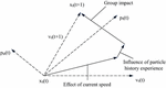
Before the beginning of the first iteration, a range of particles is usually initialized randomly in the search house and the search pace is set randomly for the particles. Each subsequent generation is based totally on 4 elements, which are the most appropriate function of the particle’s individual historic experience, the modern-day function of the particle, the world’s greatest role amongst all particles, and the uncertainty perturbation generated with the aid of the particle’s individual surroundings [13]. The optimal position of the particle’s historical experience can be called the individual extreme value. The global optimal position of all particles can be referred to as the global extreme value. The particle follows the individual extreme value and the global extreme value to change its search speed and direction and then changes its position. The schematic diagram of its updated position is shown in Figure 1. The mathematical expression of the particle swarm optimization algorithm is:
| (1) | |
| (2) |
In the above equation:
vij(t+1), vij(t) – the updated particle velocity, the current particle velocity
xij(t+1), xij(t) – Particle updated position, particle current position
pij(t), pgj(t) – individual extrema, global extrema
c1,c2 – Acceleration value of particles
r1,r2 – Mutually independent random numbers on the interval [0,1]
Equation (1) is the particle speed replace formula, and Equation (2) is the particle function replace formula. Where t denotes the wide variety of particle iterations, vij denotes the speed of the ith particle in the jth dimension, and xij denotes the function of the ith particle in the jth dimension. c1 can decide the diploma of inheritance of the particle to its individual particle gold standard position, and c2 determines the diploma of inheritance of the particle to the world’s most reliable particle function [14]. pij is the character intense value, which will be up to date in accordance with the historic ultimate cost for the duration of the particle iteration. pgj is the world extremum, which will be up to date based totally on the world’s most advantageous answer searched for. The particle swarm algorithm usually constrains the pace of the particle at some stage in the new release to make sure that the particle does now not fly out of the viable domain. vij[Vmin, Vmax], Vmin is the minimum speed of the particle and Vmax is the most pace of the particle, each of which is a non-negative integer.
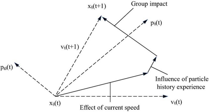
Figure 1 Velocity update and position update of particle swarm in search space.
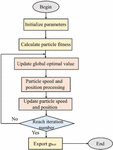
The particle swarm optimization algorithm execution technique is proven in Figure 2, and the fundamental steps of the algorithm are as follows [15]:
(1) Initialize the particle swarm via placing the measurement of c1 and c2, the variety of particles in the swarm, the most range of iterations T, the higher and decreased limits of the pace of the particles, and initialize the particle positions in the viable area and the speed inside the space constraint.
(2) Calculate the health cost of every particle through the goal characteristic to be optimized.
(3) Compare the health cost of the present-day particle with the health price of the particle’s historic greatest position. If the health cost of the modern-day particle is higher than the health fee of the particle’s historic ideal position, pbest is set to the modern-day particle’s position, and vice versa pbest stays unchanged.
(4) Compare the health cost of the present-day particle with the health price of the international ultimate role of the particle. If the health cost of the contemporary particle is higher than the health cost of the world particle gold standard position, gbest is set to the function of the modern-day particle, and vice versa gbest stays unchanged.
(5) The speed and function are up to date in accordance with Equations (1) and (2) to get the new era of particles.
(6) The role and speed of the particle are transgressed.
(7) Check whether or not the exact precision or the set variety of searches is reached, if so, give up the search and output the world extremes, if not, pass by step (2).

Figure 2 Execution flow of particle swarm optimization algorithm.
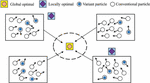
Particle swarm optimization algorithms come in two varieties: local type and global type. When all particles have access to the global extremum, the current optimal position influences each particle’s position update in the global type PSO algorithm. Each particle in the local type PSO algorithm can only access the other particles in its neighborhood, which are the particles on various edges of the topological structure graph. The architecture of the optimization algorithm’s particle population is depicted in Figure 3 [16].
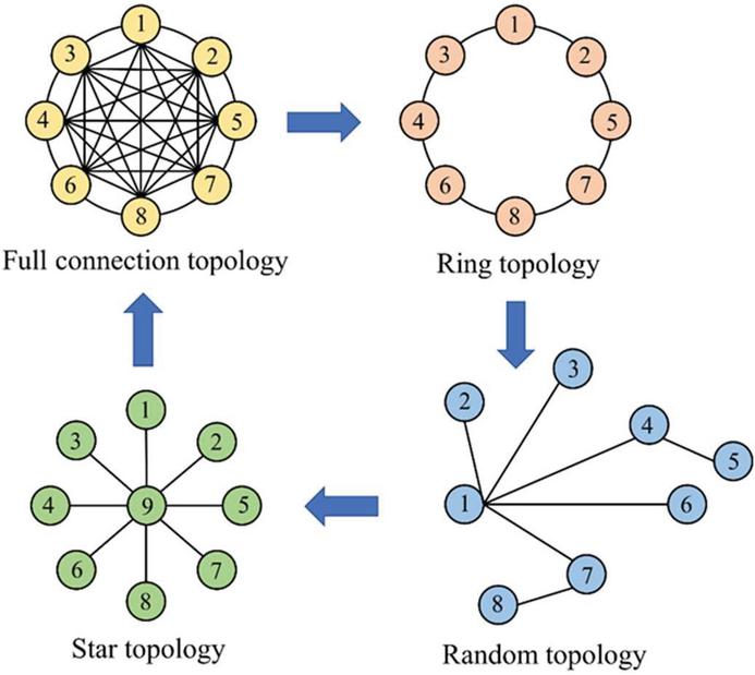
Figure 3 Topology of the particle swarm in the optimization algorithm.
2.2 Power System Multi-objective Optimization Analysis Method
In the monetary dispatch of strength system, it is integral to think about two conflicting issues of minimal financial value and minimal emission; in the trouble of venture website online selection, it is essential to reflect on consideration on no longer solely the most monetary benefit, however additionally the minimal air pollution and most social benefit, etc. This hassle is regular multi-objective optimization trouble (multi-objective optimization problem, MOP). This trouble is a normal multi-objective optimization trouble (MOP). Because the multi-objective optimization trouble is very frequent in actual existence and has robust lookup value, pupils at domestic and overseas have carried out a lot of lookups on it [17].
Multi-objective optimization problems usually consist of equation constraints or inequality constraints, and two or more objective functions. The power system multi-objective optimization problem usually satisfies the following conditions.
(1) P decision variables
| (3) |
(2) L equation constraints
| (4) |
(3) M inequality constraints
| (5) |
(4) N equation constraints
| (6) |
Where f(x) is the power objective function and xi and xi are the lower and upper bounds of the system decision variables.
The electricity gadget multi-objective optimization trouble has no most advantageous solution. The goal features are contradictory and conflicting with every other. It is not possible to attain the most effective at the same time. In the case of a higher health fee of one goal function, the answer will simply put every other goal feature in a worse state. This additionally makes the energy optimization hassle will exist many units of solutions. These options that fulfill the goal feature are referred to as possible options [18]. There is a Pareto-dominated relationship between viable options. The correlation evaluation is proven in the following figure.
(1) The Pareto principle The solution x dominates the solution y when and only when there are two sets of viable solutions, x (x1,x2,…,xp) and y (y1,y2,…,yp).
| (7) |
(2) non-dominant or non-subordinate solution When there is no x in the power system decision space such that f(x) f(x), x is referred to as a non-dominated solution or non-inferior solution.
(3) Pareto optimal We refer to x in the decision space. when it satisfies the Pareto principle.
| (8) |
(4) Pareto ideal group The set of solutions that meet the following criteria constitutes the Pareto optimum set in the minimizing multi-objective optimization problem min f(x).
(5) Pareto front (Pareto front) In the minimized power system multi-objective optimization problem min f(x) and the optimal solution set {X}, defined as
| (10) |
Using two objective functions as an example, the points in the Pareto diagram denote the solutions of the two objective functions. The non-dominated solutions are connected by black solid lines to denote the Pareto frontier. The dominated solutions are indicated by white hollow points. The Pareto optimum solution set is known as the collection of non-dominated solutions.
2.3 Improved MOPSO Algorithm Based on Multi-objective Optimization of Power System
In the multi objective dilemma of power system EED problems, objective functions struggle with each other, and the optimization of one objective may lead to the deterioration of the remaining objectives. Without changing the overall framework, MOPSO improves the selection methods of pbest and gbest in PSO based on multi-objective problems. This paper proposes an improved MOPSO algorithm, whose main functions are as follows.
(1) Determine the optimal position of individuals (P). Parsopoulos et al. [19] proposed an approach to pick the highest quality role of an individual through the usage of the Pareto dominance relation. The contemporary particle and P late in the algorithm are regularly Pareto non-dominated, which will lead to few updates of P and decrease the position of P in the algorithm. The P dedication approach is improved: the P is initialized to the preliminary function of every particle, and if the contemporary particle dominates the P, the P is up to date with the role of the contemporary particle; if the cutting-edge particle and the P can’t be compared, the quantity of dominated particles in the populace is calculated for both, and the role of the particle with the greater variety of dominated particles is chosen as the P.
(2) Determine the world’s optimum role (G). In this paper, an exterior archive set [20] is used to keep the Pareto most desirable options that have been found, and the world ideal function (G) is randomly chosen from this exterior archive set. The international finest place is selected from this exterior set with the use of a roulette wheel technique primarily based on the congestion distance of every greatest solution. As the range of iterations increases, the quantity of best solutions in this exterior set will expand rapidly, which will affect the program’s strolling pace. NC, an exterior set with variable capacity, is used, which will develop linearly from a smaller wide variety Nmin to a positive variety Nmax as the wide variety of iterations increases.
(3) Calculate the congestion distance. The crowding distance represents the sparsity of Pareto’s optimal solution. In NSGA-II, if the two adjacent individuals before and after individual (particle) B are A and C respectively, then the crowding distance of individual B is:
| (11) |
the place fi(A) and fi(C) are the i-th goal features of A and C, respectively. Here the sparsity of individual B has solely associated with its nearby measurement |fi(A) – fi(C)| in every goal function, now not to the uniformity of distribution, accordingly there is a giant challenge that the variety of options and distribution deterioration will occur, and it is challenging to converge to the Pareto the front uniformly and accurately.
(4) Setting inertial dynamic weights. The inertia weight has a very necessary effect on the convergence overall performance of the PSO algorithm, which is used to manage the impact of the historic pace of the particles on the modern speed of the particles and stability of the international detection and nearby detection overall performance of the populace [21]. Dynamic inertia weights are used to stabilize the international and nearby search of the algorithm.
| (12) |
Where: i is the cutting-edge inertia weight; max and min are the most and minimal inertia weights, respectively; g is the modern-day new release number; gmax is the most generation number.
(5) Introduction of small chance version mechanism. In the method of particle swarm evolution, a small likelihood random version mechanism is added to generate a small variety of perturbation to the particle positions to beautify the world search functionality of the algorithm via making the particles randomly perturb inside 30% of the authentic positions with a small probability. The relationship of the particle populace in the accelerated MOPSO algorithm is proven in Figure 4.
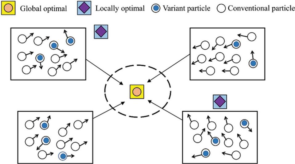
Figure 4 Classification of particle swarm optimization in MOPSO algorithm.
3 Economic Environment Dispatching Model of Power System Based on Improved Particle Swarm Algorithm
3.1 Mathematical Model for Optimal Dispatching of the Economic Environment of the Power System
The generator unit emits a large number of harmful gases during operation, with the minimum emission of polluting gases as the scheduling goal. The emission amount is related to the actual power injected into the system by each unit and is a separate functional relationship. In order to accelerate convergence, a comprehensive functional relationship with strong applicability is established.
3.1.1 The objective function of the mathematical model
(1) Fuel cost for power generation.
| (13) |
Where: Ng stands for the number of generators in the system; f1 stands for the cost of fuel for power generation; ai, bi, and ci stand for the coefficients connected to the cost of generators for power generation and are related to the consumption characteristics of the units.
(2) Pollutant gas emissions.
| (14) |
The pollutants here are SOx and NOx [22], where f2 is the pollutant emission function; i, i, i, i, i are the coefficients related to the emission characteristics of the generator.
(3) Nodal voltage offset.
| (15) |
The bus voltage degree is a necessary indicator to examine the protection of the energy gadget [23]. The voltage offset of the load node is described with the aid of . In Equation (15). K denotes the range of PQ nodes. Ui denotes the voltage magnitude of PQ node i. UiN is the rated voltage of that node. Incorporating voltage degree symptoms into planning lets in optimizing the voltage traits and enhances the protection of gadget operation.
3.1.2 Constraints of the mathematical model
(1) Power stability constraint. The energy stability equation for every node in the energy gadget shall be strictly assured that the complicated electricity injected through the generator at every node (0 for non-generator nodes) is equal to the sum of the complicated strength fed on by way of the load and the complicated strength flowing to the different nodes.
| (16) | ||
| (17) |
P and Q are the lively and reactive masses of node I respectively, where i [1, 2…Nb]; Gij, Bij, and ij i j all refer to the conductance and electronagogues between nodes i and j, respectively. They also distinguish the voltage segment angles of i and j, respectively.
(2) Unit operation constraint. Contains node voltage, generator output, and line thermal limit constraints.
| (18) | |
| (19) | |
| (20) | |
| (21) |
where P, P, Q, Q are the higher and lower limitations of energetic strength output as well as the higher and lower limits of reactive electricity output of generator i respectively; U, and U are the higher and lower limits of voltage at node i, and S and S stand for the obvious electricity at line i’s beginning and end, respectively; The starting and ending points of line i are, respectively, S and S. The top obvious energy restrictions at the start and end of the line Sfimax and Sfimin, are what are known as thermal restriction constraints. N stands for the vast range of device nodes, while N stands for the range of device lines.
3.1.3 Construction of EED optimization model
The constrained nonlinear multi-objective optimization model is constructed from the above objective function and constraints together as follows.
| (22) | |
| (23) | |
| (24) |
where: g and h are equation constraints and inequality constraints, respectively; P [P,…, P].
In the EED problem, generator gasoline value and pollutant emissions are in fighting with every other. There is no absolute most effective answer to Equation (22), so the optimization outcomes in a relatively best answer each Pareto most fulfilling set [24]. The cause of multi-objective optimization of electrical machines is to attain a set of Pareto-era scheduling optimum units that are as uniform, prolonged, and shut to the actual Pareto frontier as possible.
3.2 Improved Adaptive Multi-objective Spine Particle Swarm Optimization Algorithm
The international most suitable answer of the multi-objective algorithm for energy gadget scheduling is now not a single one, however, consists of a couple of top-quality solutions. This requires redefining the world’s most useful answer and the character’s highest quality answer of the particle population. The top-quality answer will become a set of options from a particular solution. The end result received via its optimization is a set of Pareto superior solutions or Pareto’s most efficient frontier.
In the improved MOPSO algorithm, the weight of the individual optimal solution and the global optimal solution is the same, which does not meet the requirements of the algorithm for search performance at different search stages. In order to decorate the international search functionality in the early stage of the algorithm and the nearby search functionality in the later stage, an ABBMOPSO algorithm is proposed, with the following algorithm formula.
| (25) |
The place R is a random variety of various uniformity in the vary [0,1]. , , and are the search weights decided by using the following strategies.
| (26) |
In the early stage of the algorithm, and are larger, and the international search is dominated. In the late stage of the algorithm, is large and dominated through neighborhood search. The pbest and gbest at special degrees are coordinated and the well-known deviation is progressively decreased to decrease the opportunity for untimely convergence. The probabilistic search strategy of the strength device spine particle swarm algorithm improves the accuracy and effectivity of the algorithm barring putting complicated parameters and avoids lacking the finest answer due to over-setting of parameters such as acceleration issue and inertia weights.
In the ABBMOPSO algorithm, the particle updates its role with the aid of combining its very own data and the data handed by using the world’s excellent particle. After every iteration, every particle ought to method the era scheduling ultimate solution. In the early stage of the algorithm, a new function replace formulation is utilized for the particle with the worst capacity to discover the ultimate solution, and the replace method in the early stage of the algorithm (t T/2) is as follows.
| (27) |
Later in the algorithm (t T/2) the following equation is updated.
| (28) |
Where: r is a random variety various in the vary of [0,1]; x is the contemporary international most beneficial particle position; x is the kth particle position, xkdt is now not the world foremost particle; x is the modern-day international 2d pleasant particle position, x is the particle with the worst looking for ability; T is the complete range of iterations. In the early stage of the electricity technology optimization schedule, the worst particle updates its function thru the international most suitable particle, a particle in the populace and its individual information, which has a quicker records waft and can achieve a higher search capability. In the late stage of strength technology foremost scheduling, the worst particle updates its role solely via the data of the international most useful particle and the world 2nd excellent particle, so that the function of this particle is reset to the neighborhood of the international most advantageous particle position, which can make the PSO algorithm converge to the international optimal, and this enhancement enhances the convergence velocity and the optimal-seeking potential of the MOPSO algorithm.
The steps of the ABBMOPSO algorithm for the best scheduling of strength structures are as follows.
Step 1: Randomly generate n particles, initialize the preliminary role of these n particles in the population, and the dimension of every particle is identical to the dimension of the search space.
Step 2: Process the constraint conditions, calculate the fitness of each particle, form the individual optimal value solution set and the global optimal value solution set according to the non-dominant relationship, and store the data.
Step 3: Determine the individual optimal value and the global optimal value of each particle through the dominance relationship and crowding distance.
Step 4: Combine the role and replace the system of the accelerated particle swarm algorithm to regulate the role of every particle. And decide whether or not the role satisfies the constraint, if not, the function wants to be adjusted.
Step 5: Update the exterior storage facts to save the non-dominated answer set and the dominated answer is deleted.
Step 6: Update the international most beneficial answer and the character top-of-the-line solution. The algorithm stops generation after achieving the most range of iterations or pleasant the generation requirements and returns to step two if the end-of-iteration circumstance is now not satisfied.
The strength era ideal scheduling ABBMOPSO algorithm makes use of a non-linear lowering search weight approach to optimize the replace function of the spine particle population and designs distinctive function replace techniques for the worst particles in distinctive search ranges to stability the world search functionality and nearby search functionality of the algorithm.
3.3 Generation Scheduling Model Solving Method and Selection of Compromise Optimal Solution
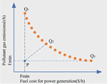
In this paper, we use the distance comparison index [25] to discover the compromise and most appropriate solution of the dispatching model. As proven in Figure 5, all factors in the parent are on the Pareto most efficient frontier, and factors Q1 and Q3 are the two excessive options with the lowest era gas price and the lowest pollutant gasoline emission, respectively. factor P is the best answer with the lowest era gasoline fee and pollutant fuel emission. However, it is not possible to attain in manufacturing practice. After identifying the factor P, the factor with the minimal Euclidean distance to P is chosen as the compromise most beneficial solution, i.e., the factor Q2. The special steps are as follows.
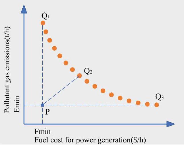
Figure 5 A method for selecting the compromise optimal solution on the Pareto optimal frontier.
Step 1: After calculating the values of the two-goal features of gasoline fee and pollutant emissions for energy generation, they are first normalized to reap the Pareto foremost frontier.
Step 2: After acquiring the Pareto most useful frontier, decide the two severe options on the Pareto most effective frontier that limit gasoline value and pollutant fuel emissions, such as factors Q1 and Q3 in Figure 5.
Step 3: Based on Q1 and Q3, draw a vertical line and a horizontal line throughout the factors Q1 and Q3, respectively, to attain an intersection point, i.e., factor P(Fmin, Emin).
Step 4: Point P is a perfect solution, which is unreachable in manufacturing practice. Using this factor as the reference point, the Euclidean distance from all options on the Pareto most efficient frontier to the reference factor P is then calculated. The answer with the minimal Euclidean distance is chosen as the compromise’s most effective solution. The components for calculating the Euclidean distance from factor P to factor Q2 are proven in Equation (29). If the Euclidean distance from P to Q2 is the smallest, then the factor Q2 is the compromise’s greatest solution.
| (29) |
4 Analysis of Algorithms for Optimal Scheduling of the Economic Environment of the Power System
4.1 Test System and Algorithm Parameter Setting
In solving the developed EED mannequin of the electricity system, the ABBMOPSO algorithm is utilized to the economic-environmental dispatch optimization calculation. To facilitate the evaluation of results, a well-known take a look at gadget with 39 IEEE nodes and 7 producing devices [26, 27] is used to operate the simulation calculation of monetary dispatch, environmental dispatch, and environmental-economic dispatch, respectively. In this case, the whole load cost of the strongest machine is 2.747pu (the baseline cost of the gadget is taken as one hundred MVA), the single line plan of the machine is proven in the literature [28], and the parameters of every producing unit (maximum and minimal output constraints and gasoline price coefficients, and pollutant fuel emission coefficients) are proven in Table 1. In order to affirm the validity and accuracy of the algorithm, a gadget optimization scheduling simulation evaluation was once carried out considering the community losses. The simulation used to be achieved on a pc outfitted with Intel(R) Core(TM) i7-10750H and sixteen GB RAM with Windows 10 running system, and Matlab 9.9 was once used for the simulation calculations.
Table 1 Parameter index of each generator set
| Unit | Pmax | Pmin | a | b | c | d | e |
| Number | (MW) | (MW) | ($/h) | ($/MWh) | ($/MWh) | ($/h) | (rad/MW) |
| 1 | 60 | 10 | 0.2 | 1.8 | 0.012 | 100 | 0.048 |
| 2 | 80 | 10 | 0.2 | 1.5 | 0.04 | 120 | 0.047 |
| 3 | 100 | 10 | 0.1 | 1.8 | 0.06 | 140 | 0.045 |
| 4 | 120 | 10 | 0.2 | 2.0 | 0.08 | 160 | 0.041 |
| 5 | 150 | 10 | 0.2 | 2.1 | 0.10 | 180 | 0.038 |
| 6 | 120 | 10 | 0.1 | 1.0 | 0.04 | 160 | 0.042 |
| 7 | 100 | 10 | 0.2 | 1.5 | 0.015 | 140 | 0.046 |
4.2 7-unit System Model Solving and Result Analysis
4.2.1 Economic dispatch and environmental dispatch optimization analysis
In the method of strength machine dispatch optimization, the energetic output of the producing unit is solved when the value of energy era is the lowest and when the emission of polluting gases is the lowest, respectively. The wide variety of particles is 50 and the widest variety of iterations is 500, and the consequences are in contrast with these of different literature as properly as MOPSO and BBMOPSO algorithms. The MOPSO is the simple multi-objective particle swarm algorithm with linear reducing inertia weights. The BBMOPSO is the simple multi-objective spine particle swarm algorithm. The replacement method of Equation (29) is adopted.
The optimal splitting point can be selected based on the network loss calculation results and considering the principles of safety and reliability, so as to make the grid configuration and distribution reasonable and improve the power consumption. The economic scheduling results considering network losses are obtained through simulation with Matlab software programs, as shown in Table 2(Best cost). The power generation cost under ABBMOPSO algorithm operation is 588.12 US dollars per hour, and the calculated economic cost is the smallest. The pollutant emission is 0.207t/h, which is lower than the backbone particle swarm optimization algorithm IBBMOPSO.
Table 2 Calculation results of economic dispatch considering network loss
| Net | Power | |||||||||
| Loss/ | Generation | Emissions/ | ||||||||
| Algorithm | G1 | G2 | G3 | G4 | G5 | G6 | G7 | MW | Costs/($/h) | (t/h) |
| MOPSO | 36.59 | 47.25 | 68.91 | 82.36 | 108.28 | 80.44 | 69.37 | 3.65 | 638.25 | 0.196 |
| SMOPSO | 20.08 | 38.60 | 61.43 | 77.19 | 95.44 | 72.69 | 60.30 | 2.79 | 606.21 | 0.203 |
| BBMOPSO | 18.89 | 37.52 | 59.67 | 70.54 | 88.39 | 67.36 | 55.21 | 2.76 | 600.98 | 0.218 |
| IBBMOPSO | 14.62 | 35.04 | 46.39 | 65.44 | 76.80 | 57.62 | 46.05 | 2.55 | 597.24 | 0.229 |
| ABBMOPSO | 15.33 | 36.20 | 45.81 | 68.30 | 80.15 | 55.46 | 48.12 | 2.26 | 588.12 | 0.207 |
The effects of the environmental dispatch thinking about the community loss are received from the simulation calculation, as proven in Table 3 (optimal pollutant gasoline emission), the cost of pollutant gasoline emission received with the aid of the ABBMOPSO algorithm is 0.194179 t/h, which is shut to the emission effects got via the BBMOPSO algorithm and IBBMOPSO algorithm and higher than the emission values bought through the different algorithms. However, the fee of energy era got by using this algorithm is 638.60 $/h, which is a decrease from the outcomes of the above 4 algorithms. Therefore, the ABBMOPSO algorithm proposed in this paper achieves a higher most beneficial solution.
Table 3 Calculation results of environmental scheduling considering network loss
| Net | Power | |||||||||
| Loss/ | Generation | Emissions/ | ||||||||
| Algorithm | G1 | G2 | G3 | G4 | G5 | G6 | G7 | MW | Costs/($/h) | (t/h) |
| MOPSO | 38.14 | 49.20 | 66.17 | 83.55 | 106.38 | 82.59 | 70.06 | 3.87 | 649.22 | 0.209 |
| SMOPSO | 22.31 | 37.64 | 64.25 | 74.50 | 99.30 | 75.18 | 62.09 | 3.03 | 650.53 | 0.196 |
| BBMOPSO | 17.50 | 36.01 | 58.72 | 73.99 | 89.74 | 68.20 | 51.04 | 2.92 | 645.10 | 0.193 |
| IBBMOPSO | 16.28 | 32.57 | 56.02 | 74.68 | 87.30 | 69.11 | 47.26 | 2.78 | 642.88 | 0.192 |
| ABBMOPSO | 16.59 | 33.12 | 58.23 | 69.47 | 86.33 | 75.23 | 50.18 | 2.85 | 638.60 | 0.192 |
4.2.2 Analysis of Economic Environment Optimized Dispatch
In order to entirely display the effectiveness of the accelerated algorithm in this paper, the BBMOPSO algorithm, IBBMOPSO algorithm, and ABBMOPSO expanded algorithm are utilized to clear up the take a look at device underneath the two instances of thinking about community loss and no longer thinking about community loss. The simulation consequences are proven in Figures 6 and 7.
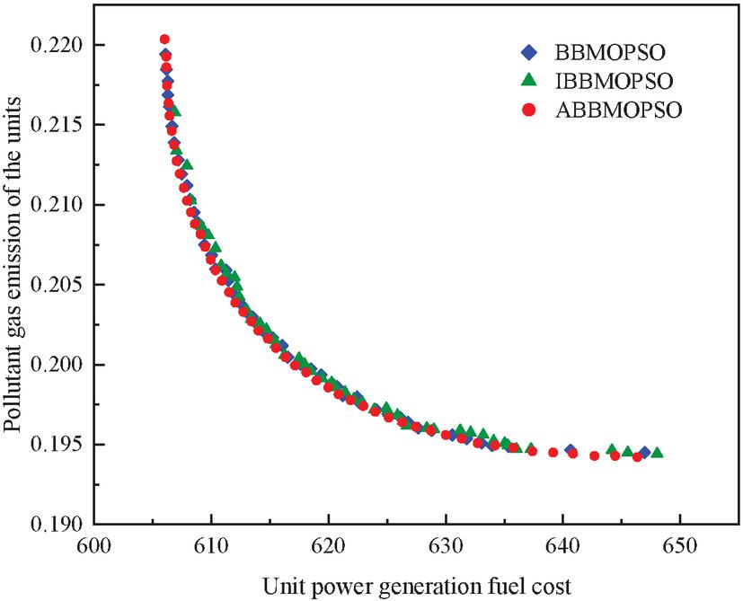
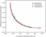
Figure 6 Comparison of Pareto’s optimal frontier considering the network loss condition.
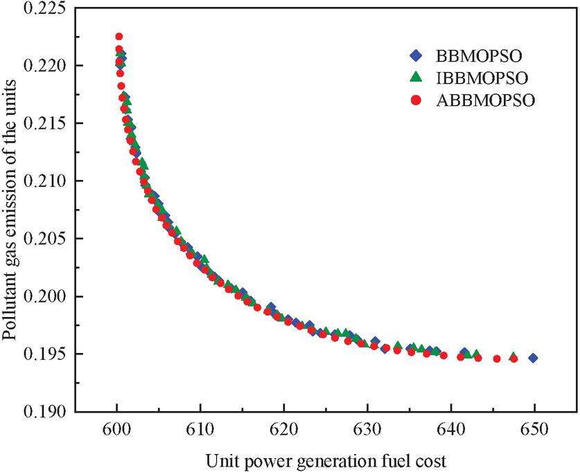
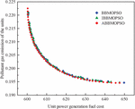
Figure 7 Comparison of Pareto’s optimal frontier without network loss.
The Pareto most appropriate frontier bought by means of the BBMOPSO and IBBMOPSO algorithms is now not uniformly distributed, while the Pareto top-quality frontier acquired by means of the ABBMOPSO algorithm proposed in this paper is smoother and greater uniform, with a wider distribution and no overlapping solutions. When reaching the Pareto optimal frontier, the power generation cost and pollution emission target function of EED can simultaneously obtain the optimal solution. The compromise most beneficial answer is chosen by means of the distance contrast index and in contrast with the effects of different algorithms. The outcomes are proven in Table 4.
Table 4 EED model compromise optimal solution
| Consider | Power | |||||||||
| Optimization | Net | Generation | Emissions | |||||||
| Algorithm | Loss | G1 | G2 | G3 | G4 | G5 | G6 | G7 | Costs ($/h) | (t/h) |
| MOPSO | Yes | 37.69 | 48.25 | 68.94 | 81.46 | 102.25 | 80.14 | 64.39 | 623.61 | 0.228 |
| BBMOPSO | Yes | 19.81 | 35.52 | 60.67 | 72.54 | 85.39 | 66.36 | 57.21 | 616.04 | 0.217 |
| IBBMOPSO | Yes | 17.62 | 36.04 | 43.36 | 64.44 | 75.80 | 56.67 | 46.08 | 599.24 | 0.223 |
| ABBMOPSO | Yes | 18.33 | 38.20 | 45.11 | 67.30 | 81.05 | 55.46 | 48.12 | 620.53 | 0.206 |
| MOPSO | No | 38.44 | 49.90 | 60.27 | 88.45 | 106.38 | 82.59 | 75.36 | 635.24 | 0.204 |
| BBMOPSO | No | 15.60 | 36.01 | 58.72 | 75.90 | 86.74 | 68.22 | 51.04 | 630.80 | 0.198 |
| IBBMOPSO | No | 16.28 | 32.57 | 55.03 | 74.68 | 87.30 | 64.37 | 47.26 | 642.88 | 0.199 |
| ABBMOPSO | No | 16.50 | 33.12 | 56.23 | 69.47 | 86.33 | 75.20 | 51.18 | 638.60 | 0.210 |
When grid loss is taken into account, the compromise ideal answer of ABBMOPSO is nice in phrases of emissions, barely greater in phrases of era price than BBMOPSO and IBBMOPSO, and higher in phrases of era fee and emissions than MOPSO. ABBMOPSO has a high-quality technology price and barely greater emissions than the different algorithms when the grid loss is now not considered. The inverse generation distance (IGD) [29] can evaluate the performance of the particle swarm optimization algorithm, and evaluate the convergence and distribution performance of the algorithm by calculating the sum of the minimum distances from the point at the real Pareto optimal frontier to the algorithm individuals. The smaller the calculation result, the better the convergence and diversity of the improved backbone multi-objective particle swarm optimization algorithm, including:
| (30) |
Where: PS is the set of factors on the actual Pareto top-of-the-line frontier; Q is the set of factors on the computed Pareto finest frontier; d(v, Q) is the minimum Euclidean distance from individual v to population Q; |PS| is the number of point sets.
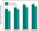
The implied value, popular deviation, and common strolling time of IGD had been calculated. The IGD outcomes are proven in Table 5, and the jogging time of the algorithm is proven in Figure 8.
Table 5 Calculation results of IGD indexes for the optimization algorithm
| Optimization | Consider | Standard | Average | ||
| Algorithm | Net Loss | IGDmax | IGDmin | Deviation | Value |
| MOPSO | Yes | 0.4557 | 0.2160 | 0.07855 | 0.3005 |
| BBMOPSO | Yes | 0.3862 | 0.2069 | 0.04734 | 0.2795 |
| IBBMOPSO | Yes | 0.2466 | 0.1722 | 0.02510 | 0.1957 |
| ABBMOPSO | Yes | 0.2039 | 0.1328 | 0.01874 | 0.1624 |
| MOPSO | No | 0.4827 | 0.2554 | 0.07235 | 0.3724 |
| BBMOPSO | No | 0.3758 | 0.2177 | 0.04738 | 0.2639 |
| IBBMOPSO | No | 0.2492 | 0.1362 | 0.02825 | 0.1972 |
| ABBMOPSO | No | 0.1935 | 0.1147 | 0.01498 | 0.1535 |
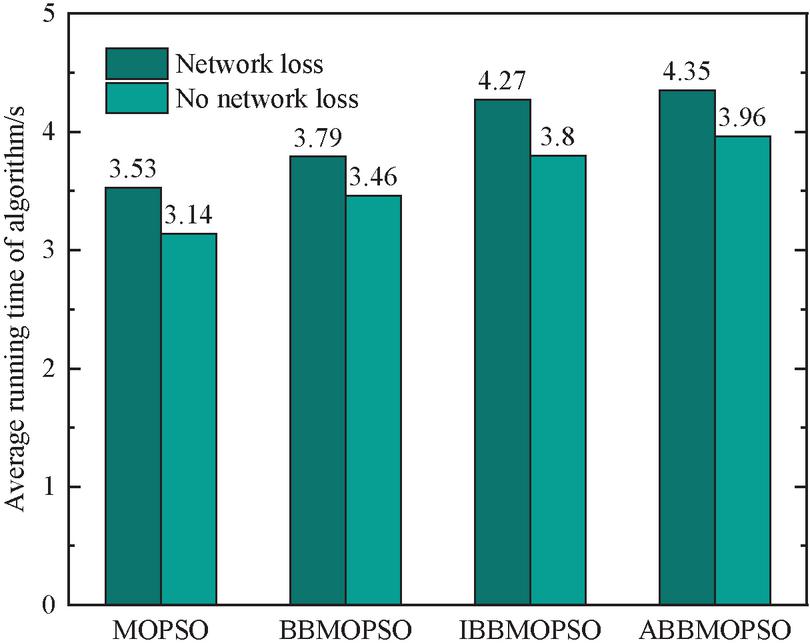
Figure 8 Running time of various multi-objective particle swarm optimization algorithms.
As proven in Table 5 and Figure 8, the suggest and general deviation acquired via the ABBMOPSO algorithm proposed in this paper are higher than these of MOPSO, BBMOPSO algorithm, and IBBMOPSO algorithm, indicating that the algorithm in this paper has apparent benefits in variety and convergence. Although the strolling time of this algorithm is barely longer than the different three algorithms, the average strolling time is very short, solely 4.35 seconds underneath the internet loss condition, which can entirely meet the operation wishes of the true EED system.
5 Conclusion
For the electric power energy industry, optimizing the unit layout and improving energy efficiency are the current primary tasks. Aiming at the economic and environmental scheduling problem of power systems, this paper proposes a solution method based on the ABBMOPSO algorithm, which satisfies the minimum power generation cost while also achieving the optimal pollutant emissions of power plants. The most important research results of this article are as follows.
(1) Firstly, the topological structure and computational flow of the particle swarm optimization algorithm are analyzed. Then, a research idea combining multi-objective optimization and the Pareto dominance principle is constructed for the scheduling problem of power generation units. The execution algorithm is the MOPSO algorithm. In the MOPSO algorithm, weight factors are used to control the degree of particle inheritance at the current speed, thereby improving the overall performance of the particle swarm optimization algorithm.
(2) The objective function in the mathematical model is to consider the fuel cost of power generation due to valve point effects, and consider nonlinear constraints such as load balancing and unit operation constraints. At the same time, an environmental function based on pollutant emissions is introduced to construct an EED model of the power system.
(3) This paper proposes an optimized ABBMOPSO algorithm, which uses a nonlinear method of reducing search weights to improve the location update technology of the backbone particle swarm, improving the global search function in the early stage and the local search ability in the later stage of the algorithm. When solving multi-objective optimal scheduling, a 7-unit standard IEEE 30-node system is used for simulation calculations. The results show that the ABBMOPSO algorithm has a minimum power generation cost of 588.1 $/h and a minimum pollutant emission of 0.192t/h, which is superior to other algorithms. The Pareto optimal frontier distribution obtained is uniform and complete.
The research in this paper can provide an alternative and effective method for the scheduling problem of energy conservation and emission reduction in power systems.
References
[1] Xin-gang Z, Ji L, Jin M, et al. An improved quantum particle swarm optimization algorithm for environmental economic dispatch[J]. Expert Systems with Applications, 2020, 152: 113370.
[2] Goudarzi A, Li Y, Xiang J. A hybrid non-linear time-varying double-weighted particle swarm optimization for solving non-convex combined environmental economic dispatch problem[J]. Applied Soft Computing, 2020, 86: 105894.
[3] Zhang Y, Li H G, Wang Q, et al. A filter-based bare-bone particle swarm optimization algorithm for unsupervised feature selection[J]. Applied Intelligence, 2019, 49: 2889–2898.
[4] Huang C, Zhou X, Ran X, et al. Adaptive cylinder vector particle swarm optimization with differential evolution for UAV path planning[J]. Engineering Applications of Artificial Intelligence, 2023, 121: 105942.
[5] Zhang Q, Li Panchi. An adaptive multi-strategy behavioral particle swarm optimization algorithm[J]. Control and Decision, 2019, 35(1): 115–122.
[6] Li W, Liang P, Sun B, et al. Reinforcement learning-based particle swarm optimization with neighborhood differential mutation strategy[J]. Swarm and Evolutionary Computation, 2023: 101274.
[7] Lu M, Guan J, Wu H, et al. Day-ahead optimal dispatching of multi-source power system[J]. Renewable Energy, 2022, 183: 435–446.
[8] Shang C, Fu L, Bao X, et al. Energy optimal dispatching of ship’s integrated power system based on deep reinforcement learning[J]. Electric Power Systems Research, 2022, 208: 107885.
[9] Rana A S, Bhagyasree B B, Harini T M, et al. Optimisation of Economic and Environmental Dispatch of Power System with and without Renewable Energy Sources[J]. Distributed Generation & Alternative Energy Journal, 2023: 491–518.
[10] Luo Z, Ma J, Jiang Z. Research on Power System Dispatching Operation under High Proportion of Wind Power Consumption[J]. Energies, 2022, 15(18): 6819.
[11] Jin J, Wen Q, Cheng S, et al. Optimization of carbon emission reduction paths in the low-carbon power dispatching process[J]. Renewable Energy, 2022, 188: 425–436.
[12] Lu Q, Chen Y, Zhang X. Smart Power Systems and Smart Grids: Toward Multi-objective Optimization in Dispatching[M]. Walter de Gruyter GmbH & Co KG, 2022.
[13] Zhang G, Xia B, Wang J, et al. Intelligent state of charge estimation of battery pack based on particle swarm optimization algorithm improved radical basis function neural network[J]. Journal of Energy Storage, 2022, 50: 104211.
[14] Li S, Chen K. Economic Operation of the Regional Integrated Energy System Based on Particle Swarm Optimization[J]. Computational Intelligence and Neuroscience, 2022, 2022.
[15] Menos-Aikateriniadis C, Lamprinos I, Georgilakis P S. Particle swarm optimization in residential demand-side management: A review on scheduling and control algorithms for demand response provision[J]. Energies, 2022, 15(6): 2211.
[16] Ghawy M Z, Amran G A, AlSalman H, et al. An Effective Wireless Sensor Network Routing Protocol Based on Particle Swarm Optimization Algorithm[J]. Wireless Communications and Mobile Computing, 2022, 2022.
[17] Sivakumar K, Jayashree R, Danasagaran K. New Reliability Indices for Microgrids and Provisional Microgrids in Smart Distribution Systems[J]. Distributed Generation & Alternative Energy Journal, 2023: 435–466.
[18] Yuan J, Cheng K, Qu K. Optimal dispatching of high-speed railway power system based on hybrid energy storage system[J]. Energy Reports, 2022, 8: 433–442.
[19] Chen Heng-An, Guan Lin, Lu Cao, et al. Multi-objective optimal scheduling model and algorithm for independent microgrid with new energy generation as the main source [J]. Power Grid Technology, 2020, 2.
[20] Liang J, Ge S-L, Qu B-Y, et al. Improved particle swarm optimization algorithm for solving economic dispatch problems of power systems[J]. Control and Decision Making, 2020, 35(8): 1813–1822.
[21] Chih M. Stochastic stability analysis of particle swarm optimization with pseudo random number assignment strategy[J]. European Journal of Operational Research, 2023, 305(2): 562–593.
[22] Wang ZQ, Dong ZT, Wang SL, et al. A two-layer optimization method for siting power emergency communication base stations considering building shading [J]. Power System Protection and Control, 2022, 50(17): 107–116.
[23] Guo Jun. Research on optimal scheduling modeling of power system based on forbidden particle swarm algorithm[J]. Electrical Engineering Technology, 2022.
[24] Naderi E, Azizivahed A, Asrari A. A step toward cleaner energy production: A water saving-based optimization approach for economic dispatch in modern power systems[J]. Electric Power Systems Research, 2022, 204: 107689.
[25] Dey S K, Dash D P, Basu M. Application of NSGA-II for environmental constraint economic dispatch of thermal-wind-solar power system[J]. Renewable Energy Focus, 2022, 43: 239–245.
[26] Wang JJ, Li W. A multi-objective feature selection method with hybrid mutual information and particle swarm algorithm[J]. Computer Science and Exploration, 2020, 14(1): 83–95.
[27] Wang S-L, Liu G-Y. A nonlinear dynamic adaptive inertia weight PSO algorithm[J]. Computer Simulation, 2021, 38(4): 249–253.
[28] Sridevi H R, Jagwani S, Kulkarni S V, et al. Frequency Control in an Autonomous Microgrid Using GA Based Optimization Technique[J]. Distributed Generation & Alternative Energy Journal, 2023: 595–610.
[29] Yin Z, Pan L, Fang X. Bio-inspired computing: theories and applications[C]//Proceedings of the 14th International Conference, BIC-TA 2019. 2019.
Biography

Gong Mengting received the bachelor’s degree in in Management Science from Xi’an University of Science and Technology in 2018. She is currently studying as a graduate student at the School of Management of Xi’an University of Science and Technology. Her research areas include energy economics and household carbon emissions.
Distributed Generation & Alternative Energy Journal, Vol. 38_5, 1609–1636.
doi: 10.13052/dgaej2156-3306.38511
© 2023 River Publishers