Study on PV Power Prediction Based on VMD-IGWO-LSTM
Zhiwei Xu1, 2,*, Kexian Xiang1, Bin Wang1 and Xianguo Li1
1School of Electrical and Information Engineering, Hunan Institute of Engineering, Xiangtan, 411104, China
2Hunan Provincial Key Laboratory of Wind Turbines and Control, No. 88, Fuxing East Road, Xiangtan City, 411104, China
E-mail: xzw@hnie.edu.cn; 1764950845@qq.com; 1227291891@qq.com; 2273329078@qq.com
*Corresponding Author
Received 19 December 2023; Accepted 27 January 2024
Abstract
This research proposes a combined approach for predicting photovoltaic power by integrating variational modal decomposition (VMD), an improved gray wolf optimization algorithm (IGWO), and long- and short-term memory neural network (LSTM) techniques. The model takes into account the impact of varying environmental factors on photovoltaic power and aims to enhance prediction accuracy. Firstly, the four environmental factors constraining the PV output power are decomposed into eigenfunctions (IMFs) through variational modal decomposition; then the improved gray wolf optimization algorithm is used to optimize the long and short-term memory neural network; finally, the dimensionality-reduced dataset is inputted into the LSTM neural network, and the dynamic temporal modeling and comparative analysis on the multivariate feature sequences are carried out. The results show that the VMD-LSTM model optimized by the improved Gray Wolf algorithm predicts better than the comparison models LSTM, VMD-LSTM and VMD-GWO-LSTM, and achieves the accurate prediction of time-volt power in the external environmental changes.
Keywords: Photovoltaic power prediction, gray wolf optimization algorithm, long- and short-term memory neural networks, variational modal decomposition.
1 Introduction
The randomness and intermittent nature of PV power generation necessitates the forecasting of PV for grid management. Because the output of photovoltaic power generation is affected by weather conditions, its power generation fluctuates greatly, which may pose challenges to the stable operation and safe dispatching management of the power grid. Through photovoltaic forecasting, the power output of photovoltaic power plants can be obtained in advance, so as to better predict and cope with the volatility of photovoltaic power generation. In this way, the power grid manager can carry out reasonable scheduling and operation according to the forecast results to ensure the stable operation of the power grid. Predictive models and algorithms can be modeled by taking into account factors such as historical data, weather forecast data, and PV cell module characteristics to improve the accuracy of forecasts. Such forecasts can help grid managers better plan and manage power supply, improving grid reliability and efficiency [1–5]. Domestic and foreign research in PV power generation prediction is more active, mainly in the following aspects: Modeling: Currently, the methods used mainly include physically based models and machine learning based models. Machine learning-based models have been widely used in recent years. Data preprocessing: The data needed for PV power generation prediction mainly include meteorological data, solar radiation data, power station information data, etc. In order to improve the accuracy of data prediction, the data need to be processed and analyzed. In order to improve the prediction accuracy, the data need to be processed. Aspects of prediction accuracy: The prediction accuracy is improved by means of model fusion, feature selection, parameter optimization and so on. Literature [6] selected environmental historical data such as solar radiation intensity, temperature, relative humidity and barometric pressure, and carried out PV power prediction by Long Short Term Memory (LSTM) neural network, which proved that the LSTM model has the ability to predict PV power. Literature [7, 8] uses Deep Belief Networks (DBN) for load prediction and LSTM learns faster and has better global convergence compared to LSTM model. It shows that the LSTM model is more robust in predicting PV power compared to other models. Literature [9] Empirical Mode Decomposition (EMD) used to process the raw data, and the processed data are input into the training model, which effectively improves the prediction accuracy [10]. The analysis discusses the advantages of Variational Mode Decomposition (VMD) over EMD in terms of mode mixing and decomposition of data, which improves the smoothness of PV series. [11] analyzes and discusses the advantages of Variational Mode Decomposition (VMD) over EMD in terms of modal aliasing and data decomposition, which improves the stationarity of PV sequences. The advantage of CEEMDAN is that there is no averaging error when decomposing. In literature [12], researchers used Particle Swarm Optimization (PSO) to optimize the weights and biases of neural networks. By this method, the drawbacks of time-consuming and poor accuracy faced by the traditional manual selection methods are overcome, thus reducing the prediction time and error. Literature [13], researchers used the Sparrow Search Algorithm (SSA) to optimize the LSTM model to better match the input data with the network structure. To this end, this paper proposes a model that introduces an improved heuristic optimization algorithm, Improvement Grey Wolf Optimizer (IGWO), into PV power prediction, which is able to achieve parameter optimization of the LSTM model under the premise of guaranteeing the prediction accuracy, and it has a better performance compared to Grey Wolf Optimizer (GWO) in terms of its global optimization. Compared with the Grey Wolf Optimizer (GWO), it has a stronger global optimization capability, higher accuracy, and is easy to implement and adjust [14, 15]. It is easy to implement and adjust.
2 Rationale and Methodology
Using the Pearson correlation coefficient, it is possible to analyze the extent to which various environmental factors affect PV power generation [16].
In Table 1, solar irradiance has the greatest impact on PV power, relative humidity and atmospheric pressure are negatively correlated with the power data and have some impact on power output, and the relative impact of air temperature is relatively small, so they are chosen as the four environmental factors that constrain PV power output.
Table 1 Environmental factors and photovoltaic power correlation coefficient
| Environmental | Solar | Relative | Atmospheric | |
| Factor | Irradiance | Temp | Humidity | Pressure |
| Ratio | 0.96 | 0.12 | 0.38 | 0.11 |
Firstly, the four environmental factors constraining the PV output power are decomposed into eigenfunctions (IMFs) by means of variational modal decomposition (vmd); then, IGWO was used to optimize the control variables of the LSTM model; finally, the dimensionality-reduced dataset is inputted into LSTM model, and the multivariate single-output feature sequences are modeled to achieve the short-term prediction of the PV power. In this test, the IGWO-optimized PV power prediction method has better prediction performance compared to the unoptimized LSTM model and the GWO-optimized LSTM model.
2.1 Specific Steps of Variational Modal Decomposition
VMD is highly efficient in handling non-stationary sequences [17]. By adaptively estimating the mode shapes and frequencies, VMD can effectively separate different mode shapes in a signal, providing valuable representations for further analysis or processing. Its core concept revolves around constructing and solving variational problems. Through an iterative optimization process, VMD successfully extracts the modal components and their frequency information from the signal, enabling a meaningful representation for subsequent analysis or processing. Compared with traditional signal decomposition techniques such as Fourier decomposition, wavelet decomposition, and empirical mode decomposition. Aliasing and artifacts of the signal can be effectively suppressed to provide more accurate signal decomposition results, and an appropriate number of eigenfunctions (IMFs) can be selectively selected according to the characteristics of the signal, so as to better adapt to the frequency and amplitude changes of the signal. Eigenfunctions (IMFs) have a good physical meaning, and each IMF represents a transient mode of the signal, which can better understand and interpret the characteristics of the signal. In terms of running speed, compared with other signal decomposition methods, VMD has lower computational complexity and faster running speed. It achieves this by adaptively estimating the mode shapes and frequencies present in the signal, and through an iterative optimization process, the VMD separates out the different mode shapes to provide a meaningful representation for further analysis or processing, and this flexibility makes the VMD a powerful tool for working with non-stationary sequences and extracting valuable information from the signal. Through VMD, the signal can be down-weighted, i.e., decomposed into different modes, so as to better understand and analyze the characteristics of the signal. The raw power time series of a photovoltaic power plant is a non-stationary signal , and it is assumed that the raw power time series is decomposed into modal components with a fixed center frequency and a finite sum of bandwidths minimized. By combining these constraints, the VMD achieves a decomposition that accurately represents the signal characteristics of the different modes, a method that effectively separates the different frequency components while maintaining the overall energy distribution of the original signal. The constraints are as follows:
| (1) |
Where: is the set of all modes obtained from the decomposition of the original signal; is the fixed center frequency corresponding to ; is the time variable; is the Dirac function; is the decomposed sequential modal AM and FM signals; is the PV prediction data.
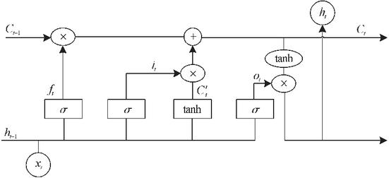
Figure 1 LSTM neural network structure.
2.2 Long Short-Term Memory Neural Network (LSTM)
LSTM is a type of control with three key control mechanisms: forgetting gates, input gates and output gates, in addition to this, LSTM uses a memory cell called cell state to transfer and store long-term memory information. Through these gate control mechanisms, LSTM can effectively deal with the long-term dependency problem and capture long-term contextual information in the sequence data [18]. LSTM is an improvement on the Recurrent Neural Ntworke (RNN), which solves the problem of long-term series and gradient dispersion of RNNs by introducing a gate mechanism and an internal memory cell. The long time series and gradient dispersion problems of RNN are solved by introducing the gate mechanism and internal storage unit. The LSTM neural network cell consists of input gate , output gate o, forgetting gate and cell state . The structure of LSTM neural network is as follows:
The data transfer formula in the LSTM neural network cell is:
| (2) |
2.3 Gray Wolf Optimization Algorithm (GWO)
GWO [19] is an algorithm for objective optimization based on how wolves behave in hunting. In wolf packs, there are four social hierarchies, which are the head wolf (), the secondary wolf (), the sub-sub-sub-wolf (), and the wolf at the bottom (). In this case, wolves are subordinate to wolves, wolves are subordinate to wolves, and wolves at the bottom are subordinate to wolves at other levels. By mimicking this social hierarchy, the GWO algorithm optimizes the objective.
Building a mathematical model: Expressing the predatory behavior of the realized wolves in a mathematical formula, we define the three optimal wolves in the pack as -wolf, -wolf, and -wolf, which act as the commanders of the pack. They renew themselves through iterative updates of the three wolves in the lead.
2.3.1 Wolf hunting modeling
Gray wolf hunting model
| (3) |
denotes the iteration, denotes the distance hunted, denotes the gray wolf’s position update formula, denotes the current optimal prey location, denotes the vector of coefficients controlling the indentation distance, and denotes the gray wolf’s attack behavior.
Coefficient vectors whose formulas are respectively:
| (4) |
, , are two random one-dimensional vectors taking values between [0, 1]. The coefficient vector is used to model the attack behavior of the gray wolf on its prey. The value of convergence factor is [0,2]. The coefficient vector provides a random weight for the prey to change the distance between the gray wolf and the prey, which is determined by the random number , so the value range of the random coefficient is [0.2].
2.4 Improved Gray Wolf Optimization Algorithm (IGWO)
The convergence factor of the gray wolf algorithm is usually controlled by adjusting the parameters. In the gray wolf algorithm, there are some key parameters that need to be set, such as the number of gray wolf individuals, the number of iterations, and the scope of the search domain. The choice of these parameters affects the convergence speed of the algorithm and the quality of the solution. For the gray wolf algorithm, there is no fixed and most suitable convergence factor, because the characteristics and requirements of different problems are different, and they need to be selected according to the specific situation. In general, a smaller convergence factor can speed up the convergence of the algorithm, but it may also cause the algorithm to fall into a local optimal solution prematurely, while a larger convergence factor may cause the algorithm to converge slowly. Therefore, when using the gray wolf algorithm, you can try different convergence factor values, and evaluate the convergence factor according to the convergence speed of the algorithm and the quality of the solution, and gradually adjust the convergence factor to select the best value. In addition, it can also be combined with the setting of other parameters, such as the number of gray wolves and the number of iterations, to perform comprehensive optimization to achieve better optimization results [20].
When GWO is , the three wolves in the lead can conduct random search to areas other than the target value, which reflects the global search capability of GWO. When , Wolf, Wolf and Wolf continuously indent towards the target value, reflecting the local search ability of GWO. Therefore, the monotone decreasing convergence factor in the original algorithm cannot fully reflect the search process of GWO algorithm, so it is necessary to improve the convergence factor [21].
In practice, the optimization process needs to constantly reduce the Search space. In order to achieve this indent search process, the Golden Section Search method is adopted in this paper. GSS combines the golden section coefficient with the sine function to optimize the search operator of GWO [22]. At the same time, the Euclidean distance calculation method based on step size is introduced.
2.4.1 Elite reverse learning mechanisms
Jumping out of the local optimum, random features can be added or perturbations can be added in practical applications. Opposition-Based Learning (OBL) can increase the diversity and quality of gray wolf populations. Reverse learning strategies have been used to improve many kinds of algorithms. Elite Opposition-Based Learning (EOBL) is the improvement of OBL to solve that the reverse solution generated by OBL in the actual application process is not necessarily better than the current search space. In evolutionary algorithms, the use of elite individuals can improve the quality and speed of population convergence, while EOBL helps to introduce more diversity. By combining these two groups, the algorithm can increase the exploration ability of the solution space.
Assuming that the average individual in the current wolves corresponds to its own extreme point as the elite individual, , a solution at the tth iteration in dimension i. The inverse solution is , .
Defined as:
| (5) |
denotes the information of the solution in dimension before reverse learning, the information of the solution in dimension after reverse learning, is a number on the interval [0.1], and and are the upper and lower bounds of the decision variables in dimension .
2.4.2 Improving the convergence factor
Traditional convergence factors do not reflect the actual optimization search process. This is because the convergence speed can vary at different stages of the optimization search process. In this paper, the convergence factor based on the change of cosine’s law is used, which can better adapt to the actual convergence situation, and its modified expression is as follows:
| (6) |
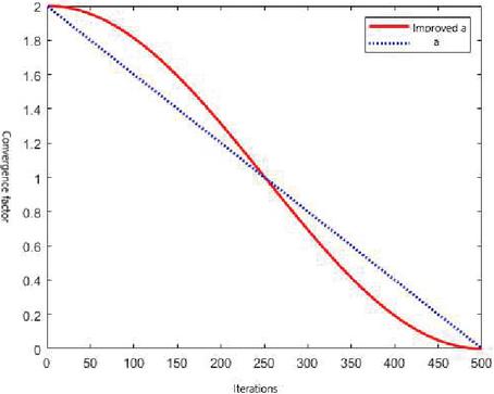
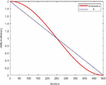
is the current iteration number, indicates the max number of iterations, and denotes the decreasing exponent, . See Figure 2 for the change chart.
Figure 2 Convergence factor iteration plot.
As can be seen from Figure 2, compared with the image of the original convergence factor, the improved convergence factor , which can balance the global and local search ability of GWO, makes decrease slower at the beginning of the iteration to make up for the defects of GWO so that the model has a better global search performance, and decreases faster at the later stage of the iteration to improve the algorithm’s search accuracy.
2.4.3 Golden sine algorithm (Gold-SA)
The unit circle embrace has a special relationship with the sine function, the gray wolf algorithm, , , are two one-dimensional random number vectors taking values in the interval of [0,1], Combining the circle and sinusoidal relations with these two random vectors, , is indicates that an arbitrary number in [0.2], is indicates that an arbitrary number in [0.]. By using sinusoidal function paths, the Gray Wolf algorithm can explore the search space in a curvilinear fashion, rather than simply moving in a straight line direction. This can increase the algorithm’s diversity in the solution space and improve global search. The use of sinusoidal function paths allows the GWO to better avoid falling into local optima and increase the chances of finding a globally optimal solution. In addition, the indentation factor calculated using the golden section coefficient is used as a fixed step to update the direction and distance. The golden section coefficient is a commonly used parameter in optimization algorithms to help balance the trade-off between global and local search. By using a fixed step size, the algorithm can update at a certain rate during the search process to avoid a search process that is too fast or too slow. The golden sine algorithm combined with the gray wolf algorithm as a global operator updates the position of the wolves after each iteration.
The following is a model of the gray wolf algorithm for wolf trapping optimized by the golden sine function
| (7) |
where is indicates that an arbitrary number in [0.2], is indicates that an arbitrary number in [0.] and . The indentation coefficients are computed to be 0.764 and 0.236.
2.4.4 Introducing a dynamic weighting strategy
| (8) |
where W1, W2, and W3 represent the learning rates of wolves against , , and wolves, respectively. The method of calculating Euclidean distance based on step size is simple and easy to implement. By calculating the distance between each gray wolf and the gray wolf of the leadership layer, a relatively simple distance matrix can be obtained, which simplifies the calculation process of the learning rate Wi. It is able to reflect the relative distance between gray wolves, so as to dynamically adjust the learning rate Wi during algorithm iteration. This dynamic adjustment helps to maintain the dynamic balance of the wolf pack in the search process, and improves the search efficiency and convergence speed of the algorithm. It is also possible to dynamically adjust the learning rate Wi based on the number and relative position of the gray wolves in the pack. This makes the GWO algorithm highly adaptable when dealing with problems of different scales and complexities. It can also cause competition between gray wolves in the pack. This competition helps to stimulate the wolf’s ability to explore and innovate, so as to find better solutions in the search process.
3 VMD-IGWO-LSTM Modeling
3.1 Model Building
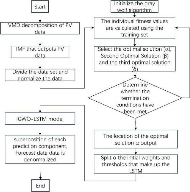
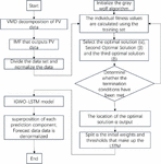
For photovoltaic power prediction, a photovoltaic prediction model based on VMD-IGWO-LSTM was proposed. The reliability of model prediction is highly correlated with the model structure setting and the selection of hyperparameters of the neural network. In this paper, IGWO is selected to optimize the LSTM model. The optimized target hyperparameters include the number of hidden layers, initial learning Xi rate, training time, batch size, and drop rate [15]. The steps to optimize an LSTM neural network using IGWO are as follows.
(1) Preprocess the data to be input, and for missing or anomalous data, use the average of the seven data before and after as a substitute.
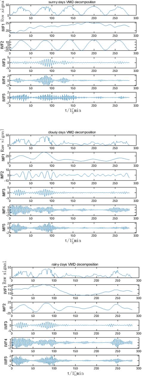
(2) The PV sequence dataset is passed through vmd to obtain the imf of each component of the PV sequence dataset.
(3) Optimize the number of hidden layers, the initial learning rate, the number of training times, the batch size, and the discard rate of the LSTM model using the gray wolf optimization algorithm. The upper parameter limit [256 0.01 300 128 0.9] and the lower parameter limit [16 0.0001 100 16 0]. The model training process was optimized using Adam’s algorithm.
(4) The data decomposed by variational modal decomposition is fed into LSTM model optimized by the GWO.
3.2 Evaluation of Forecasting Models
Root Mean Square Error (RMSE), Mean Absolute Error (MAE), Mean Absolute Percentage Error (MAPE), were selected as the criteria for evaluating the accuracy of each prediction model [23] and its expression is:
| (9) |
Where: is the actual power value at the ith point and is the predicted power value at the ith point.
RMSE measures the difference between the predicted and true values of the model, which takes into account both the magnitude and the positive and negative direction of the error. Therefore, RMSE is more sensitive to outliers, and the smaller the value of RMSE, the better the model fit. MAE measures the average absolute difference between the predicted and true values of the model, which is more concerned with the absolute value of the prediction error. Unlike RMSE, MAE is relatively insensitive to outliers because it uses the absolute difference rather than the squared difference. the smaller the value of MAE, the smaller the average error in the model’s predictions. MAE measures the average percentage error of the model’s predicted values relative to the true values, which is more comparable for data of different sizes. Because of the percentage error, MAPE is normalized for data of different sizes, making comparisons between different data more fair. MAPE is usually used for forecasting tasks with high business demands, and can better reflect the business impact of the model.
4 Model Testing
4.1 Data Sources
The four environmental data of irradiance, ambient temperature, relative humidity and atmospheric pressure in the measured power of a photovoltaic power plant in Inner Mongolia from January 1 to December 31, 2019, as well as the data acquired by the sensors of this power plant, are selected, and the abnormal data in the data are smoothed and replaced by taking the average of the seven data before and after the abnormal data. The sampling time period was from 6:45 to 19:30, the sampling interval was 15 min, and there were 52 sampling points in total, and the data of sunny day on July 4 and cloudy day on July 12 were used as the test data.
4.2 Predicted Results
Four models and the accuracy of the same models in predicting PV power for different weather conditions were compared. The four models include:
Model 1: Traditional LSTM neural network. This model uses a conventional LSTM network for PV output power prediction.
Model 2: VMD-LSTM neural network. In this model, a VMD decomposition of the training set is first performed and the subsequences obtained from the decomposition are used as inputs to the LSTM network for prediction.
Model 3: VMD-GWO-LSTM neural network. This model decomposes the PV output power data into VMD, then use a GWO to optimized LSTM network to predict each subsequence and superimposes the predictions to get the final prediction.
Model 4: VMD-IGWO-LSTM neural network. Unlike the Model 3. The subsequences obtained by VMD decomposition of PV data are used as data, then the LSTM model is optimized by using the IGWO algorithm, which can obtain more accurate prediction results.
An experimental comparison of these four models was conducted through simulations. The results show that compared with the other models, Model 4 has the best prediction effect under the same conditions, which is closest to the actual power mention. Overall, the VMD-IGWO-LSTM model has a better accuracy improvement effect in PV output power prediction, which provides an effective method to optimize the performance of PV power generation system.
Figure 3 Algorithm flowchart.
Figure 4 Exploded view of the VMD.
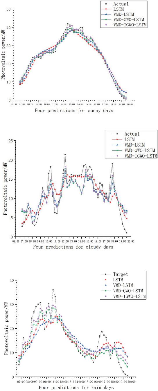
Figure 5 Comparison of four model predictions in different weather.
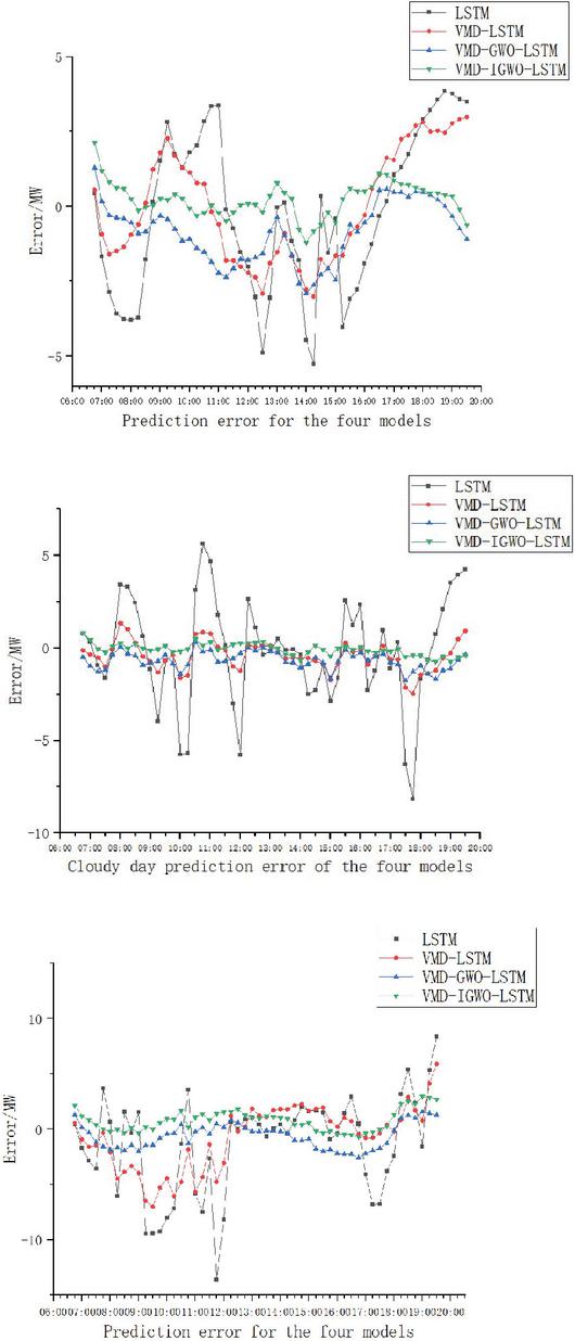
Figure 6 Comparison of prediction errors of four models in different weather.
Through Figures 5, 6, Tables 2, 3 and 4 it can be observed that that by substituting each intrinsic modal component obtained after the decomposition of the variational modes into the optimized combination model for training combination, each component can be predicted more accurately than the original sequences by the optimized combination model. A single prediction model LSTM, GWO algorithm and IGWO algorithm optimized LSTM neural network model are compared, there will be a phenomenon of over-prediction. In terms of prediction accuracy, the accuracy of the LSTM neural network optimized with the GWO and the IGWO is greatly improved, indicating that the optimization of the GWO and the IGWO improves the prediction accuracy of the model. Compared with the traditional method of manually adjusting the parameters, optimization using the GWO and the IGWO can explore the parameter space more comprehensively and can find better parameter combinations, which makes the neural network model more adapted to the characteristics of the PV power prediction task, can avoid the prediction error caused by the inaccuracy of manually adjusting the parameters, and can significantly improve the accuracy of the PV power prediction.
Tables 2, 3 and 4 show the prediction evaluation metrics of the four models, which are selected as root mean square error (RMSE), mean absolute error (MAE) and prediction error (MAPE). Based on the comparison of the prediction metrics, it can be seen that the VMD-LSTM optimized by IGWO has the highest overall prediction accuracy, and the prediction model using decomposed sequences does not exhibit obvious error transfer phenomena. From the actual data, the PV prediction has a certain lag because there is a certain time delay between the PV power generation prediction process and the actual power generation and the predicted value. This may be due to weather changes, sunshine intensity and other factors that affect the efficiency of PV power generation. That is, changes in actual power generation are not immediately reflected in the forecast. The PV output power on a sunny day is less affected by environmental factors and is more stable and can be predicted according to a regular pattern. On the other hand, the environmental factors on cloudy days change more rapidly, which leads to an increase in the difficulty of PV power prediction. As can be seen from Figure 5, the error between the test results of the model and the prediction results of the actual junction compared with the sunny day is relatively large in the case of cloudy weather conditions, partly because the sampling time interval is too large, and the data changes due to the change of cloudy clouds blocking the sun, resulting in a decrease in solar radiation. Therefore, it is necessary to reduce the sampling interval and improve the smoothness of the data, thereby improving the accuracy of the prediction.
Table 2 Four model prediction errors for sunny days
| Mould | E/MW | E/MW | E/MW |
| LSTM | 2.6405 | 2.2578 | 7.2007% |
| VMD-LSTM | 1.8466 | 1.6634 | 5.3654% |
| VMD-GWO-LSTM | 1.3189 | 1.0723 | 4.3622% |
| VMD-IGWO-LSTM | 0.62152 | 0.48874 | 1.5334% |
Table 3 Four model prediction errors for cloudy days
| Mould | E/MW | E/MW | E/MW |
| LSTM | 2.9238 | 2.2178 | 16.6838% |
| VMD-LSTM | 0.8577 | 0.66672 | 5.8907% |
| VMD-GWO-LSTM | 0.50491 | 0.41188 | 3.436% |
| VMD-IGWO-LSM | 0.31815 | 0.26585 | 2.1998% |
Table 4 Four model prediction errors for rain days
| Mould | E/MW | E/MW | E/MW |
| LSTM | 4.856 | 3.621 | 21.6% |
| VMD-LSTM | 3.11 | 2.532 | 15.8% |
| VMD-GWO-LSTM | 1.49 | 1.282 | 5.8% |
| VMD-IGWO-LSM | 1.15 | 0.881 | 4.9% |
In addition, a prediction model using decomposed sequences can decompose the PV sequences into intrinsic modal components and utilize these components for prediction. This approach can better capture the vibration modes with different frequencies and amplitudes, thus improving the accuracy of the prediction. At the same time, due to the use of a model that decomposes the sequence, the transfer of errors between the different components is not obvious, which helps to maintain the precision of the prediction. Judging from the data of photovoltaic power stations, the PV output power on sunny days is more stable less affected by environmental factors and can be predicted based on the law. The environmental factors change faster on cloudy days, which leads to an increase in the difficulty of PV power prediction. From Figures 3a and 3b. It is clear that that the model’s prediction results differ greatly in the case of large changes in weather conditions on cloudy days, partly because the sampling interval is too large and the shading of the sun by cloud cover on cloudy days leads to a decrease in the solar radiation caused by the changes in the data, so it is necessary to reduce the sampling time and improve the smoothing degree of the data so as to increase the accuracy of the prediction.
5 Conclusions
In this paper, a VMD-IGWO-LSTM prediction algorithm model is proposed, and after simulation using real data, the established model exhibits smaller values of RMSE, MSE, and MAE for short-term prediction of PV output power compared to the three prediction models, LSTM, VMD-LSTM, and VMD-GWO-LSTM. This indicates that the proposed model has a certain improvement in the short-term prediction accuracy of PV output power, which is of reference significance for the practical application.
Acknowledgments
This research was supported by Hunan Provincial Natural Science Foundation (2022JJ50122).
Conflict of Interest
We all declare that we have no conflict of interest in this paper.
Availability of Data and Materials
All data generated or analysed during this study are included in this article.
References
[1] Xue, Yang, Li, Jinxing, Yang, Jiangtian, Li, Qing, Ding, Kai. Short-term prediction of photovoltaic power based on similar day analysis and improved whale algorithm for optimizing LSTM network model [J/OL]. Southern Power Grid Technology, 1–9 [2023-11-23].
[2] Xue, Yang, Li, Jinxing, Yang, Jiangtian, Li, Qing, Ding, Kai. Short-term prediction of photovoltaic power based on similar day analysis and improved whale algorithm for optimizing LSTM network model [J/OL]. Southern Power Grid Technology, 1–9 [2023-11-23].
[3] Dai Jing, Wang Jianxiao, Zhang Zhaohua et al. Morphological characteristics and key technologies of electrically new power systems [J/OL]. New Power System, 2023, 1(2):161–183.
[4] Liu, Chen, Huang, Yihu. Research on maximum power point tracking technology for locally shaded photovoltaic [J]. Electrical Automation, 2023, 45(05): 64–66+71.
[5] Shi Y. Application of energy storage system in new energy generation system [J]. Industrial Innovation Research, 2023, (20): 96–98.
[6] Xu Libin, Cheng Ruofa, Yang Jiajing, Liu Lubing. Improved INC algorithm for rapid change of light intensity[J]. New Technology of Electrical Engineering and Electricity, 2020, 39(08): 56–65.
[7] Alaas Zuhair, Eltayeb Galal eldin A., Al Dhaifallah Mujahed, Latifi Mohsen. A new MPPT design using PV-BES system using modified sparrow search algorithm based ANFIS under partially shaded conditions [J]. Neural Computing and Applications, 2023, 35 (19): 14109–14128.
[8] Guo Jinzhi, Pan Zijun, Yuan Shaojun, et al. A variable step-size MPPT algorithm based on improved conductivity increment method[J]. Electrical Drives, 2022, 52(20): 50–56.
[9] Liu Bangyin, Duan Shanxu, Liu Fei, Xu Pengwei. Maximum power point tracking of photovoltaic array based on improved perturbation observation method[J]. Journal of Electrotechnology, 2009, 24(06): 91–94.
[10] Wang Jinyu, Wang Yuxin, Wang Haisheng. Photovoltaic maximum power point tracking based on quantum CS-P&O algorithm[J]. Power Technology, 2022, 46(07): 789–792.
[11] Chepuri Venkateswara Rao; Rayappa David Amar Raj; Kanasottu Anil Naik. A novel hybrid image processing-based reconfiguration with RBF neural network MPPT approach for improving global maximum power and effective tracking of PV system [J]. International Journal of Circuit Theory and Applications, 2023, 51 (9): 4397–4426.
[12] Lv GuanXi; Bai Di. Research on MPPT control strategy based on the Perturbation observation method [J]. Journal of Physics: Conference Series, 2023, 2474 (1).
[13] Gao, Jian, Guo, Qian, Weidong. Typical fault analysis and diagnosis of photovoltaic modules based on their I-V output characteristics [J/OL]. China Test, 1–6 [2023-11-23].
[14] Ran Chengke, Xia Xiangyang, Yang Mingsheng, et al. Photovoltaic power prediction by BP network based on day type and fusion theory[J]. Journal of Central South University (Natural Science Edition), 2018, 49(09): 2232–2239.
[15] Zhou Liang, Wu Meina, Hu An. Fast modeling of photovoltaic arrays under localized shading and characterization of extreme point distribution[J]. Journal of Electrotechnology, 2021, 36(S2): 572–581.
[16] Shi Ji-Ying, Xue Fei, Qin Zi-Jian, et al. A 3-step photovoltaic maximum power point tracking algorithm[J]. Journal of Tianjin University (Natural Science and Engineering Technology Edition), 2016, 49(05): 485–490.
[17] Mirjalili S, Lewis A. The whale optimization algorithm[J]. Advances in Engineering Software, 2016, 95: 51–67.
[18] Zhao YN, Ye L, Zhu QW. Characterization and processing methods of wind abandonment anomaly data clusters in wind farms[J]. Power System Automation, 2014, 38(21): 39–46.
[19] Li Terrible Yong, Zhang Weibin, Zhao Xinzhe, et al. Improved whale algorithm to optimize support vector regression for photovoltaic maximum power point tracking[J]. Journal of Electrotechnology, 2021, 36(09): 1771–1781.
[20] Hou Shuaihu, Zhao Hui, Yue Youjun, Wang Hongjun. MPPT tracking study of photovoltaic system under localized shading based on IDBO-IP&O algorithm [J/OL]. Complex Systems and Complexity Science, 1–9 [2023-11-23].
[21] Li Hongyan, Wang Lei, An Pingjuan, Yang Zhaoxu, Zhao Tianyue, Liu Bao. Study of photovoltaic MPPT under localized shading based on improved viscous bacteria algorithm [J]. Journal of Solar Energy, 2023, 44 (10): 129–134.
[22] Guo, Kunli, Liu, Luyu, Cai, Weizheng. Research on photovoltaic multi-peak MPPT based on hybrid algorithm [J]. Power Technology, 2021, 45 (08): 1040–1043.
Biographies

Zhiwei Xu was born in Hunan, China, in 1978. He received the M.S. and Ph.D. degrees in 2006 and 2014, respectively, from the College of Electrical and Information Engineering, Hunan University (HNU), Changsha, China. He is currently a associate Professor of Mechanical Engineering with the Hunan Institute of Engineering, Xiangtan, China. His current research interests include wind power generator and its control, power electronic transformer system, special motor and control.

Kexian Xiang was born in 2000 in Hunan, China. He graduated from the School of Applied Technology of Hunan University of Engineering in 2022 and is now a graduate student at Hunan University of Engineering. His current research interests include power electronic transformer systems and photovoltaic power forecasting.

Bin Wang was born in Xiangtan, Hunan in 1997 and graduated with a bachelor’s degree from Hunan Institute of Engineering. His main research direction is new energy and smart grid.

Xianguo Li was born in Shandong, China, in 1999. He is a Master’s student at Hunan University of Engineering, Xiangtan, China in 2023. His supervisor is Zhiwei Xu, Associate Professor, Department of Mechanical Engineering, Hunan University of Engineering, Xiangtan, China, and his research interests are in the area of new energy and smart grids.
Distributed Generation & Alternative Energy Journal, Vol. 39_3, 507–530.
doi: 10.13052/dgaej2156-3306.3936
© 2024 River Publishers
