Research on Estimation Methods for State of Charge and Core Temperature of Energy Storage Lithium Batteries

Jun Su^{1, 2,}*, Hanhan Liu¹, Zhiquan Liu¹ and Chaolong Tang¹

¹School of Electrical Engineering and Automation, Xiamen University of Technology, Xiamen, 361024, China
²Xiamen Key Laboratory of Frontier Electric Power Equipment and Intelligent Control, Xiamen University of Technology, Xiamen, 361024, China
E-mail: junsu1989@163.com
*Corresponding Author

Received 09 October 2024; Accepted 28 August 2025

Abstract

The State of Charge (SOC) and thermal conditions of lithium batteries are essential factors in the Battery Management System (BMS). Precise assessment of the SOC and core temperature of lithium batteries is crucial for the development of the BMS. This study utilizes the Square Root Cubature Kalman Filter (SRCKF) method along with the electro-thermal coupled model of lithium batteries to achieve accurate estimations of the battery’s SOC and core temperature. Initially, this research determines the parameters of the electro-thermal coupled model using the Forgetting Factor Recursive Least Squares method and the Hybrid Pulse Power Characterization tests, establishing the lithium battery’s electro-thermal coupled model. In order to validate the accuracy of SRCKF estimates, simulations were carried out under conditions defined by the Urban Dynamometer Driving Schedule, comparing the accuracy of its estimations with those of the Extended Kalman Filter and the Unscented Kalman Filter under identical conditions. The simulation outcomes demonstrate that the SRCKF can precisely estimate the battery’s SOC and core temperature, thus effectively meeting the requirements of the BMS in practical application scenarios. This study utilizes the open-source experimental dataset of the LG18650HG2 lithium battery.

Keywords: LG18650HG2 lithium battery, state of charge and core temperature estimation, square root cubature kalman filter, electro-thermal coupling model.

1 Introduction

Lithium batteries are extensively utilized in domains like electric vehicles and energy storage units [1–4]. Within these sectors, the State of Charge (SOC) and the thermal conditions of these batteries emerge as essential parameters for tracking their operational status within the Battery Management System (BMS). The SOC serves as an essential measure of the charging and discharging condition of a battery. This parameter is fundamental to BMS, facilitating precise control over a battery’s charging and discharging activities. Concurrently, the temperature denotes the thermal state of the battery and is similarly critical to the BMS, as it guides thermal management procedures.

In battery operation, differences arise between the core and surface temperatures due to the more effective cooling of the surface during charge and discharge cycles. When using temperature sensors, it is common for surface readings to be lower compared to those at the core. Depending solely on surface temperature to evaluate a battery’s thermal condition may lead to a dangerous scenario, even if the surface temperature appears to be within safe operational limits. However, the core temperature surpasses the battery’s maximum operational temperature. Battery surface temperatures can be tracked using temperature sensors integrated within the BMS, while the core temperature requires a thermocouple sensor implanted into the battery’s core structure for accurate measurement. In real-world scenarios like electric vehicles and energy storage systems, to ensure battery safety, built-in sensors are not used to measure core temperature. In practical scenarios, it is not feasible to acquire SOC information of a battery directly via sensors. Because it is impossible to obtain SOC values from a battery by directly measuring them through sensors, it must be calculated by the BMS based on collected voltage and current data. Therefore, building corresponding models that use charging/discharging data and surface temperature readings from the BMS to estimate SOC and core temperature is crucial for accurately managing battery operation.

In existing research, battery electro-thermal coupling models mainly into two categories: those based on electrochemical-thermal dynamics and those using equivalent circuit-thermal approaches [5–9]. The electrochemical-thermal coupling model mainly integrates the battery’s electrochemical mechanism with thermal modeling. Although the electrochemical-thermal model provides an in-depth portrayal of the battery’s electrochemical characteristics, the model’s complexity and computational demands generally prevent its direct use in BMS. Conversely, the equivalent circuit-thermal coupling model, establishes a coupling relationship between the battery’s equivalent circuit model and the lumped parameter thermal model through the heat produced and the battery’s temperature. This category of model is a lumped parameter model with fewer parameters, facilitates derivation of state-space equations, demands lower computational effort, and can also effectively represent the battery’s physical properties, making it more applicable for practical scenarios in BMS for electric vehicles and energy storage systems. The electro-thermal coupling model used in this thesis combines a Second-order Resistor-Capacitor Equivalent Circuit Model (2RC-ECM) with a lumped parameter Dual-State Thermal Model (2STM).

While the electro-thermal coupling model can compute the core temperature of a battery directly, relying solely on the state-space equations of the electro-thermal coupling model for estimating the core temperature still lacks sufficient accuracy. Since the electro-thermal coupling model cannot directly estimate the battery’s SOC, it is necessary to combine it with corresponding algorithms for indirect calculation of the SOC. The simplest approach to estimate the SOC is through ampere-hour integration, but as an open-loop control method, ampere-hour integration tends to have significant calculation deviations and cannot promptly correct forecast errors. Therefore, in current research, more precise filtering algorithms and intelligent algorithms are used to estimate battery SOC and core temperature [10]. Among the widely studied intelligent algorithms, including Deep Learning Feed-Forward Neural Network (DLFFNN), Convolution Neural Network (CNN) and Long Short-Term Memory neural network (LSTM) [11, 12], a large amount of operational data is required as the training set, and the demands on hardware are high, rendering them unsuitable for the current practical needs of BMS. A notable filtering algorithm for estimating SOC and core temperature is the Kalman filter [13, 14], which is based on the minimum mean square error criterion and is a linear discrete system filtering algorithm that uses estimates from the previous moment and observations from the current moment to calculate the optimal state estimates for the current moment. Researchers have developed advanced versions of the Kalman filter, such as the Extended Kalman Filter (EKF), Unscented Kalman Filter (UKF) and Cubature Kalman Filter (CKF), to enable its application in nonlinear systems [15–18]. Kalman filters do not require accumulating large data sets as neural networks do, making them more suitable for the current practical needs of BMS. This study performs a simulation analysis using the Square Root Cubature Kalman Filter (SRCKF) algorithm integrated with an electro-thermal coupling model. It evaluates the estimation accuracy against that of the EKF and UKF under identical working conditions.

The layout of this paper is as follows: Section 2 introduces the electro-thermal coupling model; Section 3 explains the parameter identification for the electro-thermal coupling model; Section 4 presents the estimation principles of the battery’s SOC and core temperature using the SRCKF, along with an analysis of the simulation experiment results; Section 5 conclusions.

2 Electro-Thermal Coupling Model

This study utilizes an electro-thermal model that integrates a 2RC-ECM with a lumped parameter 2STM. Specifically, the 2RC-ECM is used to calculate the battery’s SOC, while the 2STM is utilized to calculate the core temperature of the battery.

2.1 Equivalent Circuit Model

The model representing the battery’s electrochemical behavior employs circuit components to illustrate the phenomena, forming an nth-order equivalent circuit model by connecting n parallel Resistor-Capacitor (RC) loops in series. This model replicates the polarization effects and external physical properties of batteries during charging and discharging processes. With an increase in series RC loops, the model requires more parameters to be identified, thereby enhancing its complexity. Higher-order models of three or more orders may experience overfitting during the parameter identification process, resulting in a relatively limited improvement in simulation accuracy. Based on the above discussion, this paper uses the 2RC-ECM, considering the influence of temperature by using resistance and capacitance parameters under multiple temperature conditions. The 2RC-ECM is shown in Figure 1.

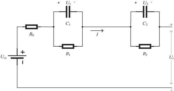
Figure 1 Schematic diagram of 2RC-ECM.

Using Kirchhoff’s principles of current and voltage, the voltage of 2RC-ECM can be expressed mathematically.

$$\{\begin{array}{c}\frac{d{U}_1}{dt}=-\frac{U_1}{R_1{C}_1}+\frac{I}{C_1}\hfill \\ \frac{d{U}_2}{dt}=-\frac{U_2}{R_2{C}_2}+\frac{I}{C_2}\hfill \\ U_t=U_{oc}-U_1-U_2-I{R}_0\hfill \\ U_{oc}=f_{ocv}(SOC)\hfill \end{array}$$

(1)

Herein, $U_{oc}$ denotes the battery’s Open Circuit Voltage (OCV), $U_t$ signifies the terminal voltage, $R_0$ represents the ohmic internal resistance, $R_1$ represents the resistance associated with electrochemical polarization, $C_1$ stands for the capacitance of electrochemical polarization, $R_2$ represents the concentration polarization resistance, $C_2$ stands for the concentration polarization capacitance. The I refers to the current of battery’s charging and discharging process, is described with a positive value for discharging and a negative value for charging in the equivalent circuit model. $U_1$ and $U_2$ correspond to the electrochemical and concentration polarization voltages, respectively.

2.2 Dual-State Thermal Model

To develop a lumped parameter dual-state thermal model for lithium batteries, the following assumptions are considered: (1) Heat is uniformly generated from the battery’s core; (2) The temperature remains consistent across the axial direction of the battery; (3) The heat only disperses outward along the radial axis. Based on these assumptions, this study employs the 2STM to characterize the thermal properties of cylindrical lithium batteries, as depicted in Figure 2.

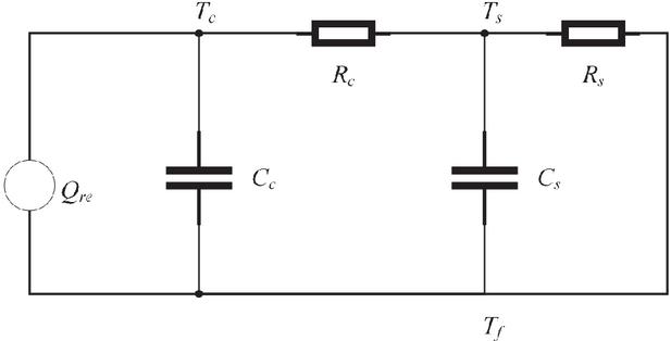
Figure 2 Schematic diagram of 2STM.

In the 2STM, the heat generated during battery operation, denoted as $Q_{re}$, and $Q_{re}$ is calculated using Bernardi’s heat generation formula, with a specific mathematical expression.

$$\{\begin{array}{c}{Q}_{re}=\underset{1}{\underbrace{\left(U_{oc}-U_t\right)I}}+\underset{2}{\underbrace{IT\frac{d{U}_{oc}}{dT}}}\hfill \\ T=\frac{T_s+T\mathrm{c}}{2}\hfill \end{array}$$

(2)

In Equation (2), the term $(U_{oc}-U_t)I$, denotes the battery’s irreversible heat, which mainly includes the Joule heat generated by ohmic resistance and the heat from polarization reactions during charging and discharging. The second part, $IT(d{U}_{oc}/dT)$, denotes the battery’s reversible heat, mainly the entropic heat change occurring within the battery electrodes. T represents the battery’s average temperature, and $d{U}_{oc}/dT$ denotes the entropic heat coefficient of the battery.

The mathematical formulation of the 2STM.

$$\{\begin{array}{c}{C}_c\frac{d(T_c-T_f)}{dt}=Q_{re}+\frac{T_s-T_c}{R_c}\hfill \\ C_s\frac{d(T_s-T_f)}{dt}=\frac{T_f-T_s}{R_s}-\frac{T_s-T_c}{R_c}\hfill \end{array}$$

(3)

Wherein, $T_c$ denotes the battery’s core temperature, $T_s$ signifies the surface temperature, $T_f$ represents the environmental temperature. $C_c$ represents the combined thermal capacity of the core, $C_s$ refers to the lumped heat capacity of the surface, $R_c$ is the equivalent thermal resistance for conduction in the core, $R_s$ describes the thermal resistance for surface convection.

2.3 Electro-Thermal Coupling Model

By integrating the 2RC-ECM and 2STM, an electro-thermal coupling model that facilitates parameter exchange can be developed. Figure 3 demonstrates the core operational concept of the presented model.

The open circuit voltage $U_{oc}$ of the battery is determined using the measured battery current $I$, and terminal voltage $U_t$, and the parameters obtained from online identification from the 2RC-ECM. The calculated $U_{oc}$ is then used in the Bernardi heat generation formula to compute the battery’s heat generation $Q_{re}$.

By inputting the battery heat generation $Q_{re}$ and environmental temperature $T_f$ into the 2STM, the battery surface temperature $T_s$ and core temperature $T_c$ at the next moment can be obtained. The battery’s working temperature is determined by calculating its average temperature $T$.

Update the parameters of the 2RC-ECM based on the working temperature T of the battery.

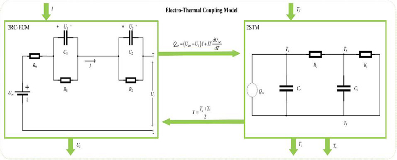
Figure 3 Electro-thermal coupling model.

3 Electro-thermal Coupled Model Parameter Identification

The electro-thermal coupled model integrates the 2RC-ECM and the 2STM through parameter exchange. To simplify the process of model parameter identification, the environmental temperature recorded during the experiment can be directly used as the battery’s working temperature. This means the 2STM would no longer need to pass the battery working temperature to adjust temperature-related parameters within the 2RC-ECM, thereby achieving the goal of decoupling the electro-thermal coupled model. After decoupling, parameter identification can be performed individually on the 2RC-ECM and 2STM. If the model was not decoupled and all parameters were attempted to be identified simultaneously, it would not only result in a significant computational load but might also result in parameters becoming unidentifiable, reducing the accuracy of parameter identification.

The experimental data used in this paper comes from the open-source experimental dataset of the LG18650HG2 type lithium-ion battery provided by the University of McMaster, Canada [19]. The LG18650HG2 battery has a standard rated capacity of 3.0Ah, a rated voltage of 3.6V, a maximum charge voltage of 4.2V, a discharge cutoff voltage of 2V, and a maximum discharge current of 20A, the standard charging current is 1.5A, while the fast charging current is 4.0A. The LG18650HG2 battery weighs 45g, with a charging temperature range of 0^∘C to 50^∘C and a discharge temperature range of $-$20^∘C to 75^∘C.

The parameters to be identified in the 2RC-ECM are $R_0$, $R_1$, $R_2$, and $C_1$, $C_2$. For the 2STM, the parameters include $R_c$, $R_s$, $C_c$, and $C_s$. The identification of model parameters utilizes the Hybrid Pulse Power Characterization (HPPC) tests from the open-source experimental dataset of the LG18650HG2.

By using the test data from the LG18650HG2 open dataset, the open-circuit voltage curve and temperature entropy coefficient curve for the LG18650HG2 can be obtained. Figure 4 shows the curve of the open circuit voltage, and Figure 5 displays the entropy heat coefficient curve.

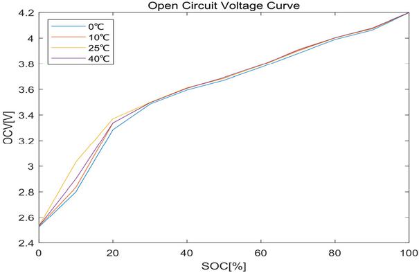
Figure 4 Open circuit voltage curve.

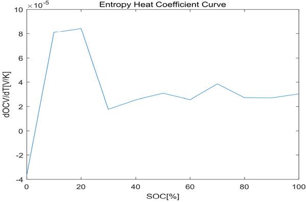
Figure 5 Entropy heat coefficient curve.

3.1 2RC-ECM Parameter Identification

Throughout the cycles of charging and discharging in a lithium battery, each model parameter undergoes continuous changes. To identify the parameters of the 2RC-ECM in real time and reduce the computational time for parameter recognition, the Forgetting Factor Recursive Least Squares (FFRLS) method is utilized for parameter identification [20]. The basic computational principle is shown in the following mathematical expression:

$$\{\begin{array}{c}{\widehat{\theta }}_k={\widehat{\theta }}_{k-1}+K_k[y_k-{\phi }_k^{\mathrm{T}}{\widehat{\theta }}_{k-1}]\hfill \\ K_k=\frac{P_{k-1}{\phi }_k}{\lambda +{\phi }_k^{\mathrm{T}}{P}_{k-1}{\phi }_k}\hfill \\ P_k=\frac{1}{\lambda }(P_{k-1}-K_k{\phi }_k^{\mathrm{T}}{P}_{k-1})\hfill \end{array}$$

(4)

Wherein, $K_k$ is the gain term, $\lambda$ is the forgetting factor, typically ranging $0.95<\lambda <1$. $P_k$ denotes the correction matrix for the predicted value at the current moment.

To achieve parameter identification of the battery model, Equation (4) of the 2RC-ECM needs to be discretized and converted it into a corresponding difference equation by applying the least squares methodology, as illustrated in Equation (9).

$\{\begin{array}{c}y=U_{oc}-U_t\hfill \\ y(k)=-{\theta }_{1}y(k-1)-{\theta }_{2}y(k-2)+{\theta }_{3}I(k)+{\theta }_{4}I(k-1)+{\theta }_{5}I(k-2)\hfill \\ \phi (k)={[-y(k-1)-y(k-2)I(k)I(k-1)I(k-2)]}^{\mathrm{T}}\hfill \\ \theta (k)={[{\theta }_1{\theta }_2{\theta }_3{\theta }_4{\theta }_5]}^{\mathrm{T}}\hfill \end{array}$

(5)

By replacing Equation (9) into Equation (4) of the FFRLS, the numerical value of $\theta (k)={[{\theta }_1{\theta }_2{\theta }_3{\theta }_4{\theta }_5]}^{\mathrm{T}}$ for the least squares form of the 2RC-ECM can be computed directly. The parameters of the 2RC-ECM, $R_0$, $R_1$, $R_2$, $C_1$, $C_2$, can be obtained through Equations (16) and (20). $\mathrm{\Delta }T$ represents the sampling time of the dataset is 0.1s.

$$\{\begin{array}{c}{R}_0=\frac{{\theta }_3-{\theta }_4+{\theta }_5}{1-{\theta }_1+{\theta }_2}\hfill \\ {\tau }_1=R_1{C}_1,{\tau }_2=R_2{C}_2\hfill \\ {\tau }_1{\tau }_2=\frac{\mathrm{\Delta }{T}^2(1-{\theta }_1+{\theta }_2)}{4(1+{\theta }_1+{\theta }_2)}=a\hfill \\ {\tau }_1+{\tau }_2=\frac{\mathrm{\Delta }T(1-{\theta }_2)}{1+{\theta }_1+{\theta }_2}=b\hfill \\ R_0+R_1+R_2=\frac{{\theta }_3+{\theta }_4+{\theta }_5}{1+{\theta }_1+{\theta }_2}=c\hfill \\ R_0{\tau }_1+R_0{\tau }_2+R_1{\tau }_2+R_2{\tau }_1=\frac{\mathrm{\Delta }T({\theta }_3-{\theta }_5)}{1+{\theta }_1+{\theta }_2}=d\hfill \end{array}$$

(6)

$$\{\begin{array}{c}{\tau }_1=\frac{b+\sqrt{b^2-4a}}{2},{\tau }_2=\frac{b-\sqrt{b^2-4a}}{2}\hfill \\ R_1=\frac{{\tau }_{1}c-{\tau }_2{R}_0-d}{{\tau }_1-{\tau }_2},R_2=c-R_1-R_0\hfill \\ C_1=\frac{b+\sqrt{b^2-4a}}{2R_1},C_2=\frac{b-\sqrt{b^2-4a}}{2R_2}\hfill \end{array}$$

(7)

The parameters of the 2RC-ECM identified by the FFRLS are shown in Figures 6, 7, 8, 9, and 10.

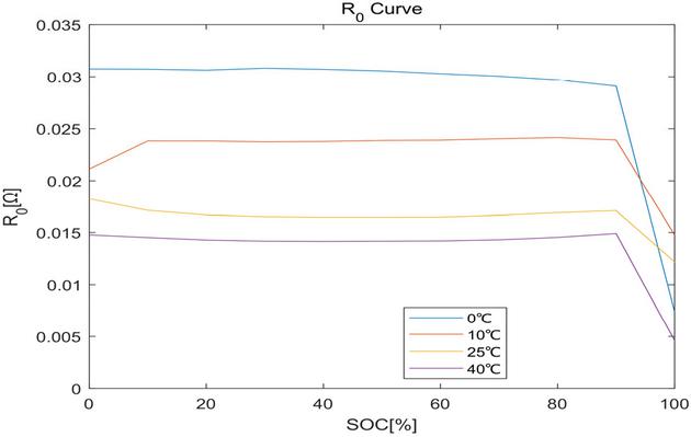
Figure 6 $R_0$ curve.

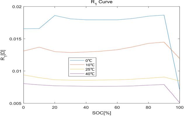
Figure 7 $R_1$ curve.

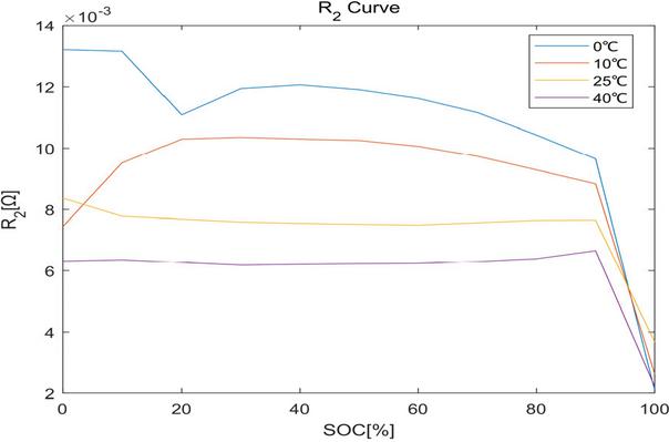
Figure 8 $R_2$ curve.

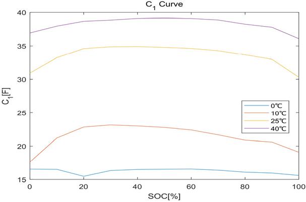
Figure 9 $C_1$ curve.

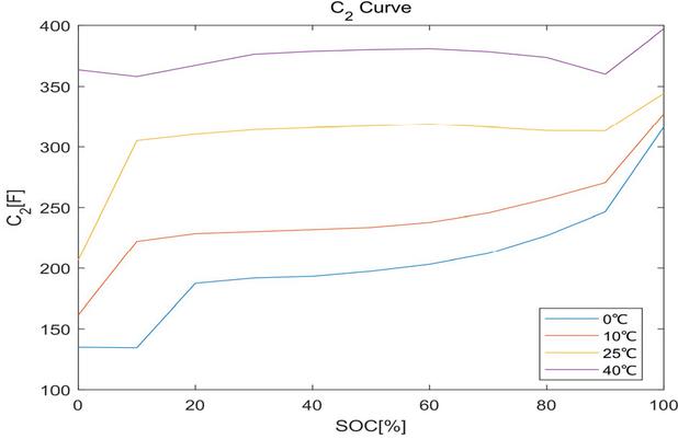
Figure 10 $C_2$ curve.

3.2 Parameter Identification of 2STM

The parameter identification of the 2STM, similar to the 2RC-ECM, also employs the FFRLS, discretizing equation of the 2STM.

$$T_c(k+1)=T_c(k)+\frac{T_s(k)+T_c(k)}{R_c{C}_c}+\frac{Q_{re}(k)}{C_c}\mathrm{\Delta }T$$	(8)
$$T_s(k+1)=T_s(k)+\frac{T_c(k)-T_s(k)}{R_c{C}_s}\mathrm{\Delta }T+\frac{T_f(k)-T_s(k)}{R_s{C}_s}\mathrm{\Delta }T$$	(9)

Throughout the entire period of sampling, the temperature of the surrounding environment stayed mostly unchanged, i.e., $T_f(k+1)=T_f(k)$. Considering the challenges in obtaining the $T_c$, the process for identifying parameters in the 2STM model was streamlined by using alternative methods, Equations (21) and (22) can be combined to eliminate the $T_c$, resulting in an expression for the $T_s$:

$T_s(k+2)$	$=\left(2-{\displaystyle \frac{\mathrm{\Delta }T}{C_s{R}_c}}-{\displaystyle \frac{\mathrm{\Delta }T}{C_c{R}_c}}-{\displaystyle \frac{\mathrm{\Delta }T}{C_s{R}_s}}\right)T_s(k+1)$
	$+\left({\displaystyle \frac{\mathrm{\Delta }T}{C_s{R}_c}}+{\displaystyle \frac{\mathrm{\Delta }T}{C_c{R}_c}}+{\displaystyle \frac{\mathrm{\Delta }T}{C_s{R}_s}}-{\displaystyle \frac{\mathrm{\Delta }{T}^2}{C_s{C}_c{R}_c{R}_s}}\right)T_s(k)$
	$+{\displaystyle \frac{\mathrm{\Delta }{T}^2}{C_s{C}_c{R}_c}}{Q}_{re}(k)+{\displaystyle \frac{\mathrm{\Delta }{T}^2}{C_s{C}_c{R}_c{R}_s}}{T}_f(k)$	(10)

The thermal capacity of the lithium battery’s outer layer, particularly the aluminum-plastic film, defines its $C_s$. The $C_s$ of the metal material remains relatively constant during usage. Therefore, the $C_s$ is derived through calculations based on the technical details provided within the manufacturer’s documentation. Given the known value of $C_s$, we only need to identify the $C_c$, $R_c$, and $R_s$. The battery heat generation $Q_{re}$ can then be calculated using the Bernardi equation. The difference equation, derived through the least squares methodology, is computed using the specific equation represented by Equation (3.2):

$\{\begin{array}{c}{T}_s(k+2)-T_s(k+1)\hfill \\ ={\theta }_1\mathrm{\Delta }{T}^2{Q}_{re}(k)+{\theta }_2\mathrm{\Delta }{T}^2(T_f(k)-T_s(k))+{\theta }_3(T_s(k+1)-T_s(k))\hfill \\ y(k)=T_s(k+2)-T_s(k+1)\hfill \\ \phi (k)={[Q_{re}(k)T_f(k)-T_s(k)T_s(k+1)-T_s(k)]}^{\mathrm{T}}\hfill \\ \theta (k)={[{\theta }_1{\theta }_2{\theta }_3]}^{\mathrm{T}}\hfill \end{array}$

(11)

Using data specified by the manufacturer, the $C_s$ is determined to be 4.5(J$\cdot$K^-1). Incorporating the dual-state thermal model’s difference equation, presented in the least squares format as Equation (29), into the FFRLS framework outlined in Equation (4), the numerical values of $\theta (k)={[{\theta }_1{\theta }_2{\theta }_3]}^{\mathrm{T}}$ can be determined. Then, using Equation (30), the values of $C_c,R_c$, and $R_s$ can be calculated.

$$\{\begin{array}{c}{R}_s=\frac{{\theta }_1}{{\theta }_2}\hfill \\ C_c=\frac{1}{{\theta }_1}\left(\frac{1-{\theta }_3}{\mathrm{\Delta }T}-\frac{1}{R_s{C}_s}\right)-C_s\hfill \\ R_c=\frac{1}{{\theta }_2{R}_s{C}_c{C}_s}\hfill \end{array}$$

(12)

The identified parameters of the 2STM based on the FFRLS are illustrated in Table 1.

Table 1 2STM parameters

Temperature [∘C]	$R_s$ [K$\cdot$W-1]	$R_c$ [K$\cdot$W-1]	$C_c$ [J$\cdot$K-1]	$C_s$ [J$\cdot$K-1]
0	1.64	2.61$\times$10-4	3.63$\times$104	4.5
10	2.93	3.51$\times$10-4	4.69$\times$104	4.5
25	4.21	2.70$\times$10-4	5.63$\times$104	4.5
40	7.42	3.90$\times$10-4	5.43$\times$104	4.5

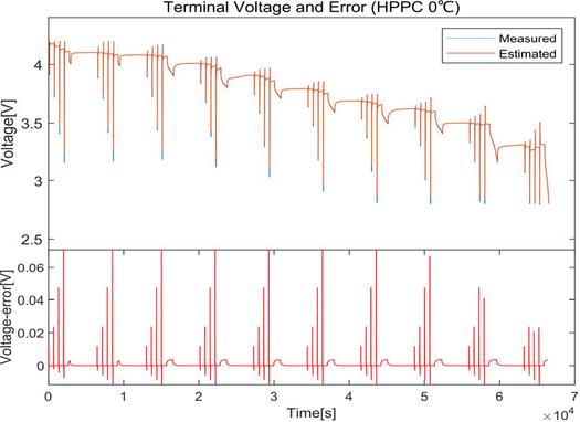
Figure 11 HPPC 0^∘C terminal voltage and error.

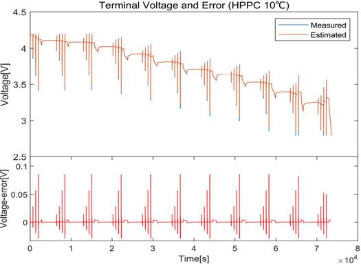
Figure 12 HPPC 10^∘C terminal voltage and error.

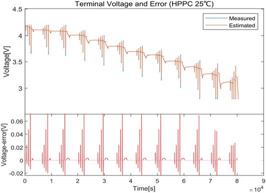
Figure 13 HPPC 25^∘C terminal voltage and error.

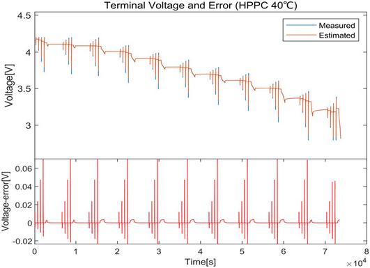
Figure 14 HPPC 40^∘C terminal voltage and error.

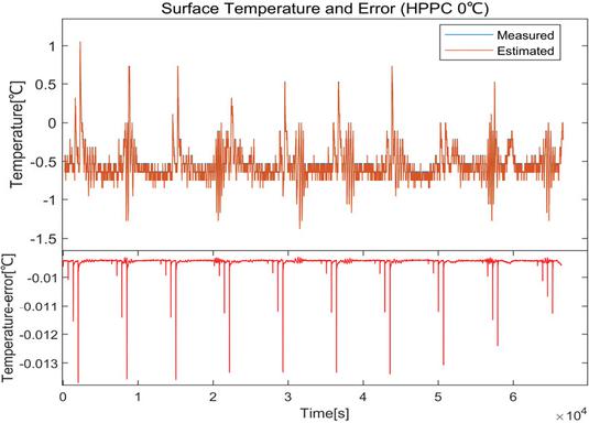
Figure 15 HPPC 0^∘C surface temperature and error.

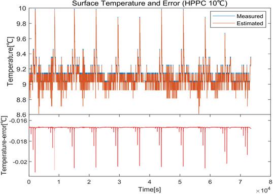
Figure 16 HPPC 10^∘C surface temperature and error.

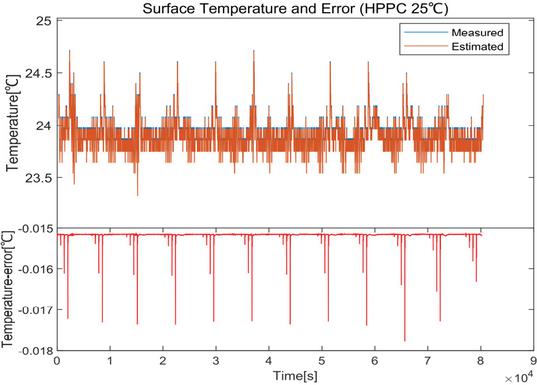
Figure 17 HPPC 25^∘C surface temperature and error.

Figure 18 HPPC 40^∘C surface temperature and error.

3.3 Model Parameter Accuracy Verification

Evaluating the precision of the electro-thermal coupling model’s parameter identification focuses on comparing predicted terminal voltage and surface temperature values against the corresponding experimental data. As the error decreases, the model’s ability to accurately identify parameters improves. The terminal voltage values obtained through measurement and estimation under HPPC conditions at ambient temperatures of 0^∘C, 10^∘C, 25^∘C, and 40^∘C, along with the associated errors, are depicted in Figures 11 to 14. Figures 15 to 18 display the measured versus predicted battery surface temperature data under HPPC testing, along with the associated error metrics. The fluctuations in terminal voltage error for the electro-thermal coupling model range from $-$0.029V to 0.086V, the maximum deviation observed in terminal voltage reached 0.086V, indicating minor discrepancies. The fluctuation range for surface temperature errors is between $-$0.0245^∘C and $-$0.0094^∘C, with a peak absolute error observed at 0.0245^∘C. Considering the discrepancies in terminal voltage and surface temperature within the electro-thermal model, it can be inferred that the parameters estimated by the FFRLS are essentially accurate.

4 Analysis of Simulation Results for Estimating Lithium Battery State of Charge and Core Temperature

Using surface temperature information gathered by the BMS, the electro-thermal model estimates core temperature directly. The estimation of core temperature relies on BMS sensor data, which can be affected by inaccuracies in surface temperature, current, and voltage readings. Additionally, the electro-thermal model is unable to derive the battery’s SOC directly from voltage and current measurements. To estimate the battery’s SOC indirectly, it integrates a modified Kalman filter method. To improve precision in estimating both the SOC and core temperature of the battery, the SRCKF algorithm can be employed in conjunction with the established electro-thermal coupling model for a more precise estimation of the battery’s SOC and core temperature. This study uses the SRCKF method in conjunction with an electro-thermal coupling model, using Urban Dynamometer Driving Schedule (UDDS) test data of the LG18650HG2 open-source experimental dataset at environmental temperatures of 0^∘C, 10^∘C, 25^∘C, and 40^∘C for the simulation testing of SOC and core temperature, and compares it with the EKF and UKF under the same conditions.

To determine the battery’s SOC and core temperature, the Kalman filter algorithm is employed after transforming the electro-thermal model into a state-space representation. This study presents two distinct sets of state equations for characterizing the electro-thermal coupling model: the first set is the electrical parameter state equation, and the second set is the thermal parameter state equation. The $I$ serves as the system input for the electrical parameter state equation, with the SOC, $U_1$ and $U_2$ as the state variables, and the $U_t$ as the system output. Similarly, the $Q_{re}$ and $T_f$ are taken as the system inputs for the thermal parameter state equation, with the $T_c$ and $T_s$ as the state variables, the $T_s$ also serves as the system output. After discretizing the two sets of state-space equations, considering the impact of model and measurement errors, and incorporating system measurement noise $v_k$, $v_{(T)k}$ and process noise $w_k$, $w_{(T)k}$. Equation (33) represents the state-space formulation for electrical variables, while Equation (36) represents the corresponding thermal variables.

$$\{\begin{array}{c}{x}_{k+1}=f(x_k,u_k)+w_k=A_k{x}_k+B_k{u}_k+w_k\hfill \\ y_k=g(x_k,u_k)+v_k=C_k{x}_k+D_k{u}_k+v_k\hfill \end{array}$$	(13)
$$\{\begin{array}{c}{x}_{(T)k+1}=f(x_{(T)k},u_{(T)k})+w_{(T)k}=A_{(T)k}{x}_{(T)k}+B_{(T)k}{u}_{(T)k}+w_{(T)k}\hfill \\ y_{(T)k}=g(x_{(T)k},u_{(T)k})+v_{(T)k}=C_{(T)k}{x}_{(T)k}+D_{(T)k}{u}_{(T)k}+v_{(T)k}\hfill \end{array}$$	(14)

In Equation (33), the state variable $x_k$, input variable $u_k$, and output $y_k$ are respectively:

$$\{\begin{array}{c}{x}_k={[SOC(k)U_1(k)U_2(k)]}^{\mathrm{T}}\hfill \\ u_k={[I(k)]}^{\mathrm{T}}\hfill \\ y_k={[U_t(k)]}^{\mathrm{T}}\hfill \end{array}$$

(15)

In Equation (36), the state variable $x_{(T)k}$, input variable $u_{(T)k}$, and output $y_{(T)k}$ are respectively:

$$\{\begin{array}{c}{x}_{(T)k}={[T_c(k)T_s(k)]}^{\mathrm{T}}\hfill \\ u_{(T)k}={[Q_{re}(k)T_f(k)]}^{\mathrm{T}}\hfill \\ y_{(T)k}={[T_s(k)]}^{\mathrm{T}}\hfill \end{array}$$

(16)

In Equations (33) and (36), the input matrix $A_k$ and $A_{(T)k}$, control matrix $B_k$ and $B_{(T)k}$, observation matrix $C_k$ and $C_{(T)k}$, transmission matrix $D_k$ and $D_{(T)k}$ in the state space equation are respectively:

$$\{\begin{array}{c}{A}_k=\left[\begin{array}{ccc}1& 0& 0\\ 0& e^{\frac{-\mathrm{\Delta }t}{R_1{C}_1}}& 0\\ 0& 0& e^{\frac{-\mathrm{\Delta }t}{R_2{C}_2}}\end{array}\right]\hfill \\ B_k=\left[\begin{array}{c}-\frac{\eta \mathrm{\Delta }t}{C_m}\\ R_1(1-e^{\frac{-\mathrm{\Delta }t}{R_1{C}_1}})\\ R_2(1-e^{\frac{-\mathrm{\Delta }t}{R_2{C}_2}})\end{array}\right]\hfill \\ C_k=[f_{ocv}(SOC)-1-1]\hfill \\ D_k=[-R_0]\hfill \end{array}$$

(17)

$$\{\begin{array}{c}{A}_{(T)k}=\left[\begin{array}{cc}1-\frac{\mathrm{\Delta }t}{R_c{C}_c}& \frac{\mathrm{\Delta }t}{R_c{C}_c}\\ \frac{\mathrm{\Delta }t}{R_c{C}_s}& 1-\frac{\mathrm{\Delta }t}{R_c{C}_s}-\frac{\mathrm{\Delta }t}{R_s{C}_s}\end{array}\right]\hfill \\ B_{(T)k}=\left[\begin{array}{cc}\frac{\mathrm{\Delta }t}{C_c}& 0\\ 0& \frac{\mathrm{\Delta }t}{R_c{C}_s}\end{array}\right]\hfill \\ C_{(T)k}=[01]\hfill \\ D_{(T)k}=[00]\hfill \end{array}$$

(18)

Herein, $C_m$ is the rated capacity of the LG18650HG2 battery, which is 3Ah. $\eta$ is the Coulomb efficiency of the LG18650HG2 battery, typically 100%. $\mathrm{\Delta }t$ is the sampling time of the dataset, which is 0.1s.

4.1 Principle of Square Root Cubature Kalman Filter Algorithm

The CKF algorithm utilizes spherical-radial cubature for Gaussian integration, applying cubature points to estimate state mean and covariance amidst additional system noise. The transformation of random variables through nonlinear functions yields an accurate approximation of their probability distribution. In the traditional CKF approach, it is essential for the covariance matrix to maintain both positive definiteness and symmetry during iterations. During the computation with the traditional CKF, applying square root and inverse operations to the covariance matrix can lead to a loss of its positive definiteness and symmetry, thereby causing errors in the CKF during the iteration process.

To address the issue where the covariance matrix potentially losing its positive definiteness and symmetry during CKF computations, and to enhance the algorithm’s robustness, the SRCKF method is enhanced by incorporating concepts from square root filtering techniques. The SRCKF approach applies QR decomposition, an orthogonal triangular method, to derive the square root of the covariance matrix, mitigating the issue of losing positive definiteness and symmetry during computation, thereby ensuring the continuity of SRCKF during the iteration process.

The steps involved in executing the SRCKF algorithm are listed below:

(1) Initialize the system state and specify the structure of the covariance for estimation errors.

$$\{\begin{array}{c}{\widehat{x}}_0=E(x_0)\hfill \\ P_0=E[(x_0-{\widehat{x}}_0){(x_0-{\widehat{x}}_0)}^{\mathrm{T}}]\hfill \\ {\widehat{x}}_{(T)0}=E(x_{(T)0})\hfill \\ P_{(T)0}=E[(x_{(T)0}-{\widehat{x}}_{(T)0}){(x_{(T)0}-{\widehat{x}}_{(T)0})}^{\mathrm{T}}]\hfill \end{array}$$

(19)

(2) Calculate the cubature points.

$$[1]=\{\left(\begin{array}{c}1\\ 0\\ \mathrm{⋮}\\ 0\end{array}\right),\left(\begin{array}{c}0\\ 1\\ \mathrm{⋮}\\ 0\end{array}\right),\mathrm{\dots },\left(\begin{array}{c}0\\ 0\\ \mathrm{⋮}\\ 1\end{array}\right),\left(\begin{array}{c}-1\\ 0\\ \mathrm{⋮}\\ 0\end{array}\right),\left(\begin{array}{c}0\\ -1\\ \mathrm{⋮}\\ 0\end{array}\right),\mathrm{\dots },\left(\begin{array}{c}0\\ 0\\ \mathrm{⋮}\\ -1\end{array}\right)\}$$

(20)

$$\{\begin{array}{c}{P}_k=S_k{S}_k^{\mathrm{T}}\hfill \\ {\zeta }_j=\sqrt{\mathrm{n}}{[1]}_j\hfill \\ X_{j,k}=S_k{\zeta }_j+{\widehat{x}}_k,j=1,2,\mathrm{\dots },2n\hfill \\ P_{(T)k}=S_{(T)k}{S}_{(T)k}^{\mathrm{T}}\hfill \\ X_{(T)j,k}=S_{(T)k}{\zeta }_j+{\widehat{x}}_{(T)k}\hfill \end{array}$$

(21)

(3) Forward the cubature points and estimate the anticipated value for the state parameter.

$$\{\begin{array}{c}{X}_{j,k+1}^{\ast }=f(X_{j,k},u_k)\hfill \\ {\overline{x}}_{k+1}=\frac{1}{2n}\sum _{j=1}^{2n}{X}_{j,k+1}^{\ast }\hfill \\ X_{(T)j,k+1}^{\ast }=f(X_{(T)j,k},u_{(T)k})\hfill \\ {\overline{x}}_{(T)k+1}=\frac{1}{2n}\sum _{j=1}^{2n}{X}_{(T)j,k+1}^{\ast }\hfill \end{array}$$

(22)

(4) Determine the root of the forecasted error covariance structure.

$$\{\begin{array}{c}{S}_{Q,k}=\mathit{chol}(Q_k)\hfill \\ {\chi }_{k+1}^{\ast }=\frac{1}{\sqrt{2n}}[X_{1,k+1}^{\ast }-{\overline{x}}_{k+1},X_{2,k+1}^{\ast }-{\overline{x}}_{k+1},\mathrm{\dots },X_{2n,k+1}^{\ast }-{\overline{x}}_{k+1}]\hfill \\ {\overline{S}}_{k+1}=\mathit{Tria}([{\chi }_{k+1}^{\ast }{S}_{Q,k}])\hfill \\ S_{(T)Q,k}=\mathit{chol}(Q_{(T)k})\hfill \\ {\chi }_{(T)k+1}^{\ast }=\frac{1}{\sqrt{2n}}[X_{(T)1,k+1}^{\ast }-{\overline{x}}_{(T)k+1},\hfill \\ X_{(T)2,k+1}^{\ast }-{\overline{x}}_{(T)k+1},\mathrm{\dots },X_{(T)2n,k+1}^{\ast }-{\overline{x}}_{(T)k+1}]\hfill \\ {\overline{S}}_{(T)k+1}=\mathit{Tria}([{\chi }_{(T)k+1}^{\ast }{S}_{(T)Q,k}])\hfill \end{array}$$

(23)

(5) Update the cubature points.

$$\{\begin{array}{c}{X}_{j,k+1}={\overline{S}}_{k+1}{\zeta }_j+{\overline{x}}_{k+1}\hfill \\ X_{(T)j,k+1}={\overline{S}}_{(T)k+1}{\zeta }_j+{\overline{x}}_{(T)k+1}\hfill \end{array}$$

(24)

(6) Forward the cubature nodes and compute the expected observation result.

$$\{\begin{array}{c}{Y}_{j,k+1}=g(X_{j,k+1},u_{k+1})\hfill \\ {\overline{y}}_{k+1}=\frac{1}{2n}\sum _{j=1}^{2n}{Y}_{j,k+1}\hfill \\ Y_{(T)j,k+1}=g(X_{(T)j,k+1},u_{(T)k+1})\hfill \\ {\overline{y}}_{(T)k+1}=\frac{1}{2n}\sum _{j=1}^{2n}{Y}_{(T)j,k+1}\hfill \end{array}$$

(25)

(7) Determine the square root of the covariance matrix related to measurement noise.

$$\{\begin{array}{c}{\gamma }_{k+1}=\frac{1}{\sqrt{2n}}[Y_{1,k+1}-{\overline{y}}_{k+1},Y_{2,k+1}-{\overline{y}}_{k+1},\mathrm{\dots },Y_{2n,k+1}-{\overline{y}}_{k+1}]\hfill \\ S_{R,k+1}=\mathit{chol}(R_{k+1})\hfill \\ S_{\mathrm{YY},k+1}=\mathit{Tria}([{\gamma }_{k+1}{S}_{R,k+1}])\hfill \\ {\gamma }_{(T)k+1}=\frac{1}{\sqrt{2n}}[Y_{(T)1,k+1}-{\overline{y}}_{(T)k+1},\hfill \\ Y_{(T)2,k+1}-{\overline{y}}_{(T)k+1},\mathrm{\dots },Y_{(T)2n,k+1}-{\overline{y}}_{(T)k+1}]\hfill \\ S_{(T)R,k+1}=\mathit{chol}(R_{(T)k+1})\hfill \\ S_{(T)\mathrm{YY},k+1}=\mathit{Tria}([{\gamma }_{(T)k+1}{S}_{(T)R,k+1}])\hfill \end{array}$$

(26)

(8) Determine the root of the cross-variance structure.

$\{\begin{array}{c}{P}_{\mathrm{XY},k+1}={\chi }_{k+1}{\gamma }_{k+1}^{\mathrm{T}}\hfill \\ {\chi }_{k+1}={\displaystyle \frac{1}{\sqrt{2n}}}[X_{1,k+1}-{\overline{x}}_{k+1},X_{2,k+1}-{\overline{x}}_{k+1},\mathrm{\dots },X_{2n,k+1}-{\overline{x}}_{k+1}]\hfill \\ P_{(T)\mathrm{XY},k+1}={\chi }_{(T)k+1}{\gamma }_{(T)k+1}^{\mathrm{T}}\hfill \\ {\chi }_{(T)k+1}={\displaystyle \frac{1}{\sqrt{2n}}}[X_{(T)1,k+1}-{\overline{x}}_{(T)k+1},\hfill \\ X_{(T)2,k+1}-{\overline{x}}_{(T)k+1},\mathrm{\dots },X_{(T)2n,k+1}-{\overline{x}}_{(T)k+1}]\hfill \end{array}$

(27)

(9) Kalman gain.

$$\{\begin{array}{c}{K}_{k+1}=\left(\frac{P_{\mathrm{XY},k+1}}{S_{\mathrm{YY},k+1}^{\mathrm{T}}}\right)S_{\mathrm{YY},k+1}^{-1}\hfill \\ K_{(T)k+1}=\left(\frac{P_{(T)\mathrm{XY},k+1}}{S_{(T)\mathrm{YY},k+1}^{\mathrm{T}}}\right)S_{(T)\mathrm{YY},k+1}^{-1}\hfill \end{array}$$

(28)

(10) Revise the predicted state estimate and determine the root value for the updated error variance.

$$\{\begin{array}{c}{\widehat{x}}_{k+1}={\overline{x}}_{k+1}+K_{k+1}(y_{k+1}-{\overline{y}}_{k+1})\hfill \\ S_{k+1}=\mathit{Tria}([{\chi }_{k+1}^{\ast }-K_{k+1}{\gamma }_{k+1}{K}_{k+1}{S}_{R,k+1}])\hfill \\ {\widehat{x}}_{(T)k+1}={\overline{x}}_{(T)k+1}+K_{(T)k+1}(y_{(T)k+1}-{\overline{y}}_{(T)k+1})\hfill \\ S_{(T)k+1}=\mathit{Tria}([{\chi }_{(T)k+1}^{\ast }-K_{(T)k+1}{\gamma }_{(T)k+1}{K}_{(T)k+1}{S}_{(T)R,k+1}])\hfill \end{array}$$

(29)

In these equations, $E(x_0)$ represents the mathematical expectation, $Q=\mathit{diag}([{10}^{-9}{10}^{-9}{10}^{-9}])$ and $Q_{(T)}=\mathit{diag}([{10}^{-6}{10}^{-6}])$ are the process noise covariance matrices, $R=\mathit{diag}([\mathrm{1\; 1\; 1}])$ and $R_{(T)}=\mathit{diag}([{10}^{-5}{10}^{-5}])$ are the measurement noise covariance matrices. $\mathit{Tria}()$ denotes the QR decomposition of the enclosed matrix, while chol() refers to the Cholesky factorization of the matrix inside the parentheses. The initial value $x_0=[1;0;0]$ and $P_0=\mathit{diag}([{10}^{-5}{10}^{-5}{10}^{-5}])$, $P_{(T)0}=\mathit{diag}([{10}^{-5}{10}^{-5}])$.

4.2 Simulation Results and Analysis

Due to the absence of core temperature measurements in the LG18650HG2 open-source dataset, it is necessary to utilize the actual measurements of $T_f$ and $T_s$ from the LG18650HG2 dataset, along with the parameters of the electro-thermal coupling model $C_s$, $R_s$, $R_c$. According to Equation (3), the theoretical value of the core temperature is derived and evaluated against the algorithm simulation value. The simulation outcomes of the battery’s SOC and core temperature under the UDDS drive cycle at environmental temperatures of 0^∘C, 10^∘C, 25^∘C, and 40^∘C are shown in Figures 19, 20, 21, 22 and 23, 24, 25, 26.

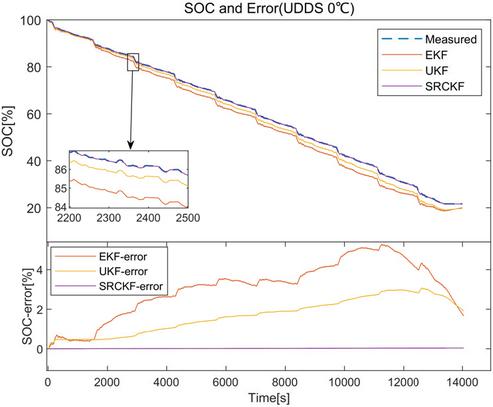
Figure 19 UDDS 0^∘C SOC and error.

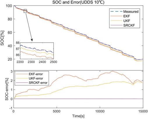
Figure 20 UDDS 10^∘C SOC and error.

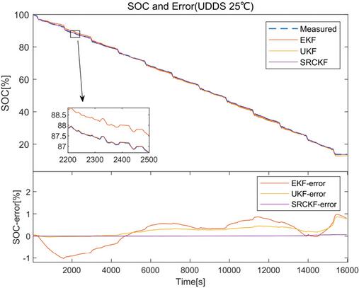
Figure 21 UDDS 25^∘C SOC and error.

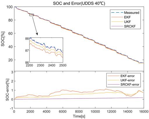
Figure 22 UDDS 40^∘C SOC and error.

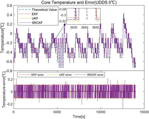
Figure 23 UDDS 0^∘C core temperature and error.

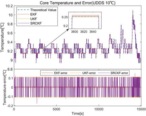
Figure 24 UDDS 10^∘C core temperature and error.

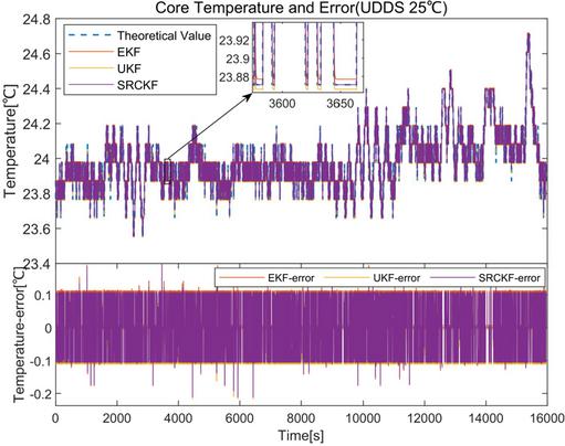
Figure 25 UDDS 25^∘C core temperature and error.

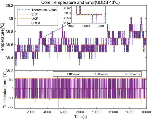
Figure 26 UDDS 40^∘C core temperature and error.

Metrics used for assessing SOC errors are outlined in Table 2.

Table 2 SOC error evaluation metrics

	Error Metrics (SOC)
Algorithm	MAE	MAPE	RMSE
EKF(UDDS 0∘C)	3.08%	7.79%	3.37%
EKF(UDDS 10∘C)	1.93%	4.27%	2.06%
EKF(UDDS 25∘C)	0.49%	1.21%	0.56%
EKF(UDDS 40∘C)	0.71%	1.71%	0.75%
UKF(UDDS 0∘C)	1.69%	4.48%	1.89%
UKF(UDDS 10∘C)	1.16%	3.09%	1.29%
UKF(UDDS 25∘C)	0.25%	0.82%	0.31%
UKF(UDDS 40∘C)	0.51%	1.37%	0.54%
SRCKF(UDDS 0∘C)	0.02%	0.02%	0.05%
SRCKF(UDDS 10∘C)	5.81$\times$10-4%	1.53$\times$10-3%	8.14$\times$10-4%
SRCKF(UDDS 25∘C)	0.01%	0.05%	0.02%
SRCKF(UDDS 40∘C)	0.09%	0.27%	0.11%

Table 3 provides an overview of metrics used for assessing errors in core temperature.

Table 3 Core temperature error evaluation metrics

	Error Metrics (Core Temperature)
Algorithm	MAE	MAPE	RMSE
EKF(UDDS 0∘C)	0.009∘C	0.122%	0.016∘C
EKF(UDDS 10∘C)	0.007∘C	0.081%	0.012∘C
EKF(UDDS 25∘C)	0.011∘C	0.047%	0.021∘C
EKF(UDDS 40∘C)	0.009∘C	0.022%	0.015∘C
UKF(UDDS 0∘C)	0.007∘C	0.106%	0.013∘C
UKF(UDDS 10∘C)	0.006∘C	0.063%	0.001∘C
UKF(UDDS 25∘C)	0.008∘C	0.034%	0.018∘C
UKF(UDDS 40∘C)	0.007∘C	0.016%	0.012∘C
SRCKF(UDDS 0∘C)	0.003∘C	0.072%	0.013∘C
SRCKF(UDDS 10∘C)	0.001∘C	0.014%	0.009∘C
SRCKF(UDDS 25∘C)	0.005∘C	0.021%	0.018∘C
SRCKF(UDDS 40∘C)	0.002∘C	0.006%	0.012∘C

Analysis of all simulation outcomes reveals that SRCKF demonstrates superior accuracy in estimating SOC and core temperature. The maximum error of SOC estimation for UDDS under four different ambient temperature conditions by SRCKF does not exceed 0.19%, and the estimated maximum deviation for core temperature does not surpass 0.28^∘C. The Mean Absolute Errors (MAE) for all SOC estimations by SRCKF doesn’t surpass 0.09%, the Root Mean Square Error (RMSE) for all SOC estimations by SRCKF doesn’t surpass 0.11%, and the Mean Absolute Percentage Error (MAPE) of all SOC estimations by SRCKF does not exceed 0.27%. The MAE of all core temperature estimations by SRCKF does not exceed 0.005^∘C, the RMSE does not exceed 0.018^∘C, and the MAPE does not exceed 0.072%. Comparative analysis indicates that SRCKF achieves an average SOC estimation accuracy improvement of 94% over UKF and 96% over EKF. SRCKF demonstrates a 58% average improvement in core temperature estimation accuracy over UKF, and 68% over EKF.

5 Conclusions

By integrating the SRCKF algorithm with the electro-thermal coupling framework, effective real-time estimation of SOC and core temperature of the battery is achieved. The outcomes from simulations, using the open-access LG18650HG2 dataset, demonstrate findings under chosen UDDS scenarios, SRCKF achieves an average enhancement of 94% and 58% in SOC and core temperature accuracy, respectively, over UKF, and an average enhancement of 96% and 68% over EKF. In comparison to conventional EKF and UKF algorithms, the SRCKF algorithm demonstrates enhanced estimation precision and greater robustness. The dataset utilized for these simulation experiments was derived from the LG18650HG2 lithium battery, with future plans for extending the testing and validation of the SRCKF algorithm to encompass various other lithium battery types.

References

[1] Peng Y, Huang F, Xie X, et al. A Predictive Approach for Lithium-Ion Battery SOH using LSTM Neural Networks Enhanced by Health Matrix Optimization. DGAEJ. Published online October 28, 2024:831-850. doi:10.13052/dgaej2156-3306.3947.

[2] Dar U, Siddiqui AS, Bakhsh FI. Design and Control of an Off Board Battery Charger for Electric Vehicles. DGAEJ. Published online April 25, 2022. doi:10.13052/dgaej2156-3306.3744.

[3] Zhou Y, Wang F, Xin T, Wang X, Liu Y, Cong L. Discussion on International Standards Related to Testing and Evaluation of Lithium Battery Energy Storage. DGAEJ. Published online November 30, 2021. doi:10.13052/dgaej2156-3306.3732.

[4] Kumar P, Das V, Singh AK, Karuppanan P. Levelized Cost of Energy-Based Economic Analysis of Microgrid Equipped with Multi Energy Storage System. DGAEJ. Published online May 18, 2023. doi:10.13052/dgaej2156-3306.38411.

[5] Chen L, Hu M, Cao K, et al. Core temperature estimation based on electro-thermal model of lithium-ion batteries. Int J Energy Res. 2020;44(7):5320–5333. doi:10.1002/er.5281.

[6] Li D, Yang L, Li C. Control-oriented thermal-electrochemical modeling and validation of large size prismatic lithium battery for commercial applications. Energy. 2021;214:119057. doi:10.1016/j.energy.2020.119057.

[7] Liu Y, Tang S, Li L, et al. Simulation and parameter identification based on electrochemical- thermal coupling model of power lithium ion-battery. Journal of Alloys and Compounds. 2020;844:156003. doi:10.1016/j.jallcom.2020.156003.

[8] Saw LH, Ye Y, Tay AAO. Electro-thermal characterization of Lithium Iron Phosphate cell with equivalent circuit modeling. Energy Conversion and Management. 2014;87:367–377. doi:10.1016/j.enconman.2014.07.011.

[9] Zhu J, Knapp M, Darma MSD, et al. An improved electro-thermal battery model complemented by current dependent parameters for vehicular low temperature application. Applied Energy. 2019;248:149–161. doi:10.1016/j.apenergy.2019.04.066.

[10] How DNT, Hannan MA, Hossain Lipu MS, Ker PJ. State of Charge Estimation for Lithium-Ion Batteries Using Model-Based and Data-Driven Methods: A Review. IEEE Access. 2019;7:136116–136136. doi:10.1109/ACCESS.2019.2942213.

[11] Vidal C, Malysz P, Kollmeyer P, Emadi A. Machine Learning Applied to Electrified Vehicle Battery State of Charge and State of Health Estimation: State-of-the-Art. IEEE Access. 2020;8:52796–52814. doi:10.1109/ACCESS.2020.2980961.

[12] Singirikonda S, Obulesu YP. Lithium-Ion Battery State of Charge Estimation Using Deep Neural Network. DGAEJ. Published online March 3, 2023. doi:10.13052/dgaej2156-3306.3833.

[13] Dai H, Zhu L, Zhu J, Wei X, Sun Z. Adaptive Kalman filtering based internal temperature estimation with an equivalent electrical network thermal model for hard-cased batteries. Journal of Power Sources. 2015;293:351–365. doi:10.1016/j.jpowsour.2015.05.087.

[14] Hu L, Hu R, Ma Z, Jiang W. State of Charge Estimation and Evaluation of Lithium Battery Using Kalman Filter Algorithms. Materials. 2022;15(24):8744. doi:10.3390/ma15248744.

[15] Xie J, Wei X, Bo X, et al. State of charge estimation of lithium-ion battery based on extended Kalman filter algorithm. Front Energy Res. 2023;11:1180881. doi:10.3389/fenrg.2023.1180881.

[16] Guo Y, Chen Y. Study on SOC Estimation of Li-ion Battery Based on the Comparison of UKF Algorithm and AUKF Algorithm. J Phys: Conf Ser. 2023;2418(1):012097. doi:10.1088/1742-6596/2418/1/012097.

[17] Tian Y, Huang Z, Tian J, Li X. State of charge estimation of lithium-ion batteries based on cubature Kalman filters with different matrix decomposition strategies. Energy. 2022;238:121917. doi:10.1016/j.energy.2021.121917.

[18] Zhang S, Zhang C, Jiang S, Zhang X. A comparative study of different adaptive extended/unscented Kalman filters for lithium-ion battery state-of-charge estimation. Energy. 2022;246:123423. doi:10.1016/j.energy.2022.123423.

[19] Naguib M. LG 18650HG2 Li-ion Battery Data and Example Deep Neural Network xEV SOC Estimator Script. Published online March 5, 2020. doi:10.17632/CP3473X7XV.3.

[20] Yu C, Huang R, Zhang Y. Online Identification of Lithium Battery Equivalent Circuit Model Parameters Based on a Variable Forgetting Factor Recursive Least Square Method. In: The Proceedings of the 16th Annual Conference of China Electrotechnical Society. Vol. 891. Lecture Notes in Electrical Engineering. Springer Nature Singapore; 2022:1286–1296. doi:10.1007/978-981-19-1532-1_136.

Biographies

Jun Su received the bachelor’s degree in electrical engineering from Staffordshire University in 2012, the master’s degree in electrical energy systems from Cardiff University in 2014, and the philosophy of doctorate degree in Electrical Engineering from Auckland University of Technology in 2020. He is currently working as an lecturer at School of Electrical Engineering and Automation, Xiamen University of Technology. His research areas include electric vehicles and new energy grid optimization, intelligent distribution network, relay protection.

Hanhan Liu received the bachelor’s degree in Electrical Engineering and Automation from North China Institute of Science and Technology in 2021. He is currently studying for a master’s degree at Xiamen University of Technology. His research areas include battery management system technology.

Zhiquan Liu received the bachelor’s degree in Electrical Engineering and Automation from Xiamen University of Technology in 2023. He is currently studying for a master’s degree at Xiamen University of Technology. His research areas include power quality monitoring.

Chaolong Tang received the bachelor’s degree in Electrical Engineering and Automation from Xiamen University of Technology in 2023. He is currently studying for a master’s degree at Xiamen University of Technology. His research areas include photovoltaic power generation technology.

Distributed Generation & Alternative Energy Journal, Vol. 41_1, 51–82
doi: 10.13052/dgaej2156-3306.4113
© 2026 River Publishers