An Adaptive Filter Algorithm Based on Hyperbolic Tangent Function for Power Quality Enhancement in Distribution Network
Jeetendra Kumar1, Salauddin Ansari1, Om Hari Gupta1, Arun Kumar Singh1 and Vijay K. Sood2,*
1National Institute of Technology, Jamshedpur, Jharkhand 831014, India
2Ontario Tech University, Oshawa, Canada
E-mail: jeetkumaree11@gmail.com; salauddinansari.ee@gmail.com; omhari.ee@nitjsr.ac.in; aksingh.ee@nitjsr.ac.in; vijay.sood@ontariotechu.ca
*Corresponding Author
Received 22 December 2024; Accepted 20 January 2025
Abstract
Static compensators (or DSTATCOMs) are commonly used in the integration of renewable energy sources (RES) into the grid to provide a variety of functions such as reactive power compensation, harmonic elimination, zero voltage regulation (ZVR), power factor correction (PFC), grid current balancing, etc. Considering the recent trends on integration of the RES to the grid, an enhanced control structure is needed. In this paper, a hyperbolic tangent function based adaptive filter (HTFAF) is applied for effective operation of the static compensator. This adaptive filter’s (HTFAF) update rule is based on a cosine function and follows the stochastic gradient descent principle. The HTFAF is used to estimate the peak values of the active and reactive segments of load current. These peak values are used to precisely determine reference grid currents. The control structure for the DSTATCOM is designed to provide harmonics-free, sinusoidal, balanced grid currents under both linear and non-linear, as well as balanced and unbalanced loads. Furthermore, the system has the ability of operate in either PFC or ZVR modes. The proposed control structure is also compared with existing control structure LMF and LMS and found to be superior. The MATLAB/Simulink environment is used for the design of a grid-connected DSTATCOM and its control logic. The performance of the system is also validated using the OPAL-RT real-time simulator.
Keywords: Power quality, DSTATCOM, distribution network, utility grid, power factor, non-linear load.
Nomenclature
| RES | Renewable energy sources |
| ZVR | Zero voltage regulation |
| PFC | Power factor correction |
| LMF | Least mean fourth |
| LMS | Least mean square |
| EPLL | Enhanced phase-locked loop |
| NN | Neural Network |
| DNLMS | Decorrelation Normalized LMS |
| PCC | Point of Common Coupling |
| DC-link voltage | |
| Line and phase voltage of the distribution network | |
| Modulation index | |
| DC-link capacitance | |
| DC-link voltage | |
| Interfacing inductance | |
| Fundamental time | |
| Resistance of the ripple filter | |
| Capacitance of the ripple filter | |
| PF | Power factor |
| V | Point of common coupling voltage |
| u, u, u | Active unit templates in phase a, b and c respectively |
| u, u, u | Reactive-unit templates in phase a, b and c respectively |
| Active weight component of the phase-a load current, | |
| Step size of the filter | |
| Scaling filter | |
| Norm penalty factor | |
| Sparse penalty factor | |
| e | Error between the phase-a load current and the fundamental load current |
| i | Current flowing through phase-a load |
| Average active weight of load currents | |
| Reactive weight component of phase ‘a’ load current | |
| Average reactive weight of load currents | |
| Loss component | |
| Proportional and integral gains of the PI controller | |
| Reference DC-link voltages | |
| Reactive loss component | |
| Net active weight of active segment | |
| Net active weight of reactive segment | |
| Active and Reactive segments of 3-phase reference grid currents | |
| , , | Reference 3-phase grid currents in phase-a, -b and -c |
| , , | Sensed 3-phase grid current in phase-a, -b and -c |
| P | Grid power |
| v, i | Grid voltage and current respectively |
1 Introduction
The unfavorable effects on the environment due to the carbon emissions, resulting from extreme use of traditional energy sources, such as oil, natural gas, coal, has pushed the energy sector to shift towards more clean and sustainable energy means [1]. Moreover, the concept of zero carbon emissions is gaining interest, which is most likely to capture the forthcoming energy market. Renewable sources like solar, wind, hydro and biomass are the best options in terms of availability and cleanliness. Power converters are the key structures, which are used to interface and integrate these RES to the utility grid [2]. The power converters in the distribution network used for grid integration are generally known as distribution static compensators (DSTATCOM), also known as active power filters. Therefore, proper control of DSTATCOM is necessary to achieve the required objectives [3]. Power quality issues are dominant in the distribution network, which must be addressed effectively [4]. The DSTATCOMs are configured to mitigate multiple power quality issues at a time. Moreover, DSTATCOMs are also used for integrating the electric vehicles and establishing power transfer between the vehicle and grid, broadly known as vehicle-to-grid and grid-to-vehicle application.
Numerous control schemes have been suggested in the literature, demanding their efficiency in meeting various objectives [5]. Broadly, the control techniques are divided into either frequency-based or time-based. Some of the frequency-based algorithms include Fourier Series [6], Discrete Fourier Transform [7], Fast Fourier Transform, Recursive Discrete Fourier Transform, Kalman Filter-based algorithms [8], etc. Likewise, some of the time-based control techniques are power balance theory, single-phase PQ theory [9], single-phase DQ theory, least mean square (LMS) [10], least mean fourth (LMF) [11], enhanced phase-locked loop (EPLL) based algorithm [12], etc. Owing to the simple structure, time-based algorithms are usually utilized for power quality enhancement. On the other hand, frequency-based algorithms exhibit more complex structures which result in sluggish performance. Additionally, the burden on the processor is comparatively lesser in the case of time-based algorithms than frequency-based ones.
Based on the synchronous reference frame theory, the PLL-based algorithm is commonly utilized for DSTATCOM operation, which performs satisfactorily under ideal grid conditions. However, under abnormal grid conditions such as voltage distortion, sags, and swells, the performance deteriorates. Therefore, PLL-less control structures with advanced system performance are attracting control engineers. Typically, the loads on the distribution network are highly nonlinear and unpredictable, which necessitates estimating load requirements. Therefore, fast and precise evaluation of the peak of load currents is becoming inevitable. The Neural Network (NN) based structures are considered as most efficient structures, the weights of which are updated during each sampling period. Consequently, the peaks of load currents are estimated with the help of NN-based structures with various weight update rules. With fixed step size, leaky LMS [13], LMS [14], and Decorrelation Normalized LMS (DNLMS) [15] have been reported in the literature. A small step size helps achieve the result with a reduced steady-state error. However, it results in sluggish system performance. On the contrary, a significant step size enhances the speed of estimation and, at the same time, increases the steady-state error. A variable step-size leaky LMS control has been presented in [16]. Various NN-based control algorithms have been reported with a similar concept in the literature. In some cases, for achieving balanced sinusoidal grid currents, the fundamental positive sequence components from the load currents and grid voltages are estimated using adaptive filters [17]. An NN-based adaptive linear element-LMS logic is implemented on the distribution static compensator used for integration of wind energy conversion system [18]. In [19], a mixed step size normalized least LMF scheme is used for DSTATCOM integrated electric vehicle station. For achieving fast convergence rate, a modified proportionate affine projection algorithm is proposed for DSTATCOM [20]. A widely linear reduced complexity quaternion LMS adaptive control logic is suggested for PV-DSTATCOM [21]. Another adaptive technique known as Wiener variable step size, is proposed for PV-DSTATCOM in [22].
Broadly, generalized integrator (GI) based adaptive filters such as second-order generalized integrator (SOGI) [23], third-order generalized integrator [24], modified SOGI [25] have been used for this purpose. A Kalman filter-based control structure has been suggested in [25]. Likewise, a complex coefficient filter is utilized for power quality enhancement in grid-connected inverters [26]. Recently, a model predictive control technique has been introduced for grid integration. The NN-based control algorithms are the simplest and have the best dynamic performance from the previously discussed control scheme. Although the control techniques have been provided satisfactory performance, these control techniques need improvement to provide better performance in terms of accuracy and performance speed. Moreover, the control technique must be robust in terms of handling disturbances.
Considering the design of robust control logic for DSTATCOM, control structure including hyperbolic tangent function-based adaptive filter (HTFAF) structure is presented in this article. The design characteristics of the adaptive filter are as follows.
• The filter structure’s update rule originated from a logarithmic-hyperbolic cosine function-based cost function by implementing a stochastic gradient descent concept [27].
• The derivation is based on minimizing the cost function, which is based on the error signal.
• The HTFAF is used for estimating the peak of the load currents, which determines the load requirement by the system.
The control structure is designed by focusing on the following objectives:
1. Fast and accurate calculation of load current components (active and reactive).
2. Rejection of harmonics from grid currents to achieve total harmonics distortion of the grid current below the limit specified in IEEE 519 standard [24].
3. For achieving balanced grid currents even when the unbalanced load is applied to the system.
4. Regulating the DC-link voltage to ensure that the system performs at a desirable level.
5. For operating the DSTATCOM in PFC mode.
6. For operating the DSTATCOM in ZVR mode.
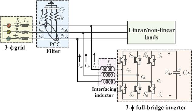
Figure 1 Block diagram of 3-phase grid consociated DSTATCOM.
The control structure is designed for 3-phase grid interfaced DSTATCOM. For software simulation, MATLAB/Simulink environment is preferred. The control structure is designed to operate the system separately under PFC mode or ZVR mode. Linear and nonlinear loads are connected to the system for verifying the performance of the control scheme. Comparative performance of HTFAF is presented with LMS and LMF under unbalanced nonlinear load. Simulated results of the system are observed under balanced and unbalanced linear as well as nonlinear loads and voltage sag.
2 Configuration of Test System
The block diagram of a 3-phase grid interfaced static compensator is shown in Figure 1. The loads are attached to a 3-phase source and DSTATCOM. Depending on the nature of the load, the loads can draw either linear or nonlinear currents. Most of the domestic loads draw nonlinear currents due to their electronic nature. The harmonics contents in the load currents have detrimental effects on the power system equipment. Harmonics are responsible for causing electromagnetic interference in nearby communication networks and heating in the transformers.
The reactive power and harmonics are supplied through a capacitor-supported 3-phase full-bridge inverter. The inverter operates as DSTATCOM and offers reactive power compensation. The DSATCOM is attached at the Point of Common Coupling (PCC) along with filtering elements. For meeting the purpose of supplying ripple-free currents, interfacing inductors are used. Ripple filters are employed at the PCC to eliminate voltage sags.
3 Design of Test System
The rating of DSTATCOM is dependent on the reactive power it must supply. Depending on the reactive power rating, the DC-link voltage, DC-link capacitor, ripple filters, and interfacing inductors are designed. Here, the design parameters are considered for designing a DSTATCOM for compensating a load of 25 kVA at 0.8 pf.
3.1 DC-link Voltage Calculation
The DC-link voltage is dependent on the voltage of the 3-phase grid, which is considered as 415 V. The DSTATCOM’s DC-link voltage is set to be greater than double the peak of phase voltage. Thus, based on the distribution network’s voltage, the DC-link voltage is computed as,
| (1) |
where is the DC-link voltage, is the line voltage of the distribution network, and m is the modulation index.
3.2 DC-link Capacitor Calculation
The DC-link capacitor is dependent on the maximum allowable DC link voltage ripple and switching frequency.
| (2) |
Considering (variation of energy during dynamics) as 10% 0.1, ‘’ (DC link voltage) as 700 V and ‘’ as 680 V, ‘a’ (overloading factor) as 1.2, ‘t’ as 35 ms, ‘I’ as 34.78 A, now after putting this value in (1), the DC-link capacitor comes out to be,
| (3) |
3.3 Calculation of Interfacing Inductor
The inductor used for an interface is decided by the switching frequency and the maximum current ripple allowed via the inductor. It is calculated as,
| (4) |
Considering ‘m’ as 1, ‘’ as 700 V, ‘b’ as 1.2, ‘’ as 5 kHz, and current ripple as 15% of the phase current. Therefore, the interfacing inductor comes out to be,
| (5) |
3.4 Calculation of Ripple Filters
The ripple filter is a high pass filter of first-order with a tuning frequency of half that of the switching frequency. The ripple filters are meant to remove the noise from the PCC voltages. For effective operation of ripple filters, the time constant must be significantly less as compared with the fundamental time () as,
| (6) |
It can be considered that .
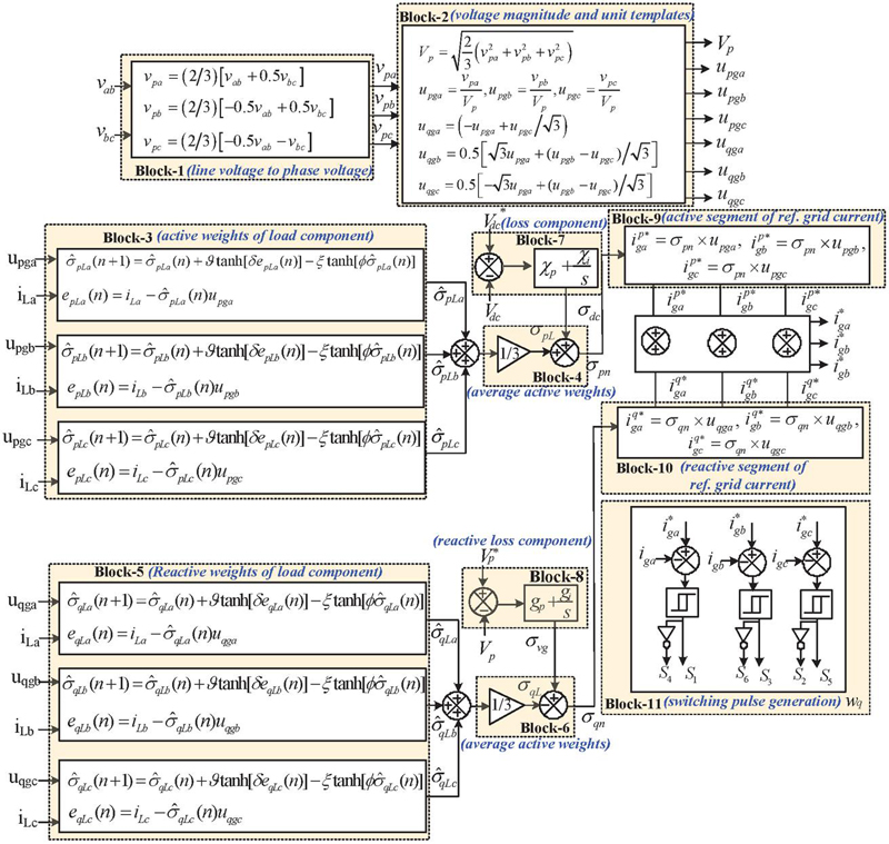
Figure 2 Control logic for grid interfaced inverter highlighting each part of calculation involved in generating the switing pulses for inverterWhere is the resistance, is the capacitance of the ripple filter, and is the period of the switching pulse. Considering the switching frequency as 5 kHz and as 5 , the is obtained as 5 F.
4 Control Structure for Grid Connected DSTATCOM
Static compensators are the grid-connected inverters, which are substantially utilized for connecting renewable sources into the grid. The significant advantages of these compensators include reduction of harmonics, reactive power compensation, balancing of grid currents, etc. Depending on the required mode of operation, they are configured to achieve PFC at the grid side or ZVR. During the system’s operation in PFC mode, only the active power is drawn, and the reactive power is zero. The power factor (PF) on the utility grid is quite close to unity. On the contrary, in ZVR mode, reactive power is drawn along with the active power to stabilize the PCC voltage, which is required for the satisfactory performance of the system. The overall control structure for both modes is shown in Figure 2. The design procedure follows the following steps.
4.1 Determination of Unit Templates
In the first step, the active and reactive segments of the unit vectors are determined, which are in-phase and in quadrature, respectively, with the grid voltages. The line voltages (v, v) are perceived at the PCC and the phase voltages (v, v, v) are calculated as highlighted in Block 1 of Figure 2 and the equations are given as per [29],
| (7) | |
| (8) | |
| (9) |
The value of PCC voltage (V) is calculated as highlighted in Block 2 of Figure 2 and the equation is given as,
| (10) |
The unit templates are determined as highlighted in Block 2 of Figure 2 and equations are given as follows,
| (11) |
The in-phase or active unit templates (u, u, u) are in-phase with the grid voltages. The reactive or quadrature-unit templates (u, u, u) are calculated with the help of the in-phase unit templates (u, u, u) as highlighted in Block 2 of Figure 2 and equations are given as follows,
| (12) | |
| (13) | |
| (14) |
These unit templates, are employed to calculate the reference active and reactive segments of grid currents.
4.2 Estimation of Active and Reactive Load Component
The HTFAF is utilized to estimate the active and reactive weight components of load currents highlighted in Block 3 and Block 5) of Figure 2. The HTFAF is based on single-layer NN logic, consisting of input and output layers. The filter’s inputs are the currents flowing through the load. The load components are the weights of the neurons. The weight update rule of HTFAF [27] is written as,
| (15) |
Where, is the active weight component of the phase-a load current, is the step size of the filter, is the scaling filter, is the norm penalty factor and is the sparse penalty factor. The norm penalty factor is less than or equal to the multiplication of step size () and scaling filter ().
The e is the error between the phase-a load current and the fundamental load current or the output, which can be written as,
| (16) |
where i is the current flowing through phase-a load.
The weight is calculated based on the error value. The weight is calculated considering the error minimization logic. Likewise, the weights of phases ‘b’ and ‘c’ are determined as,
| (17) |
and
| (18) |
where and are the active weights of the ‘b’ and ‘c’ phase load currents, and are the error values that can be written as,
| (19) | |
| (20) |
where and are the load currents of ‘b’ and ‘c’ phases,
Now, the average active weight of load currents is estimated as highlighted in Block 4 of Figure 2 and equation is given as,
| (21) |
Like the determination of the active weight component of the load current, the reactive weight component of the load current is also calculated highlighted in Block 5 of Figure 2. The reactive weight component of phase ‘a’ load current () is calculated as,
| (22) |
where is the error signal in phase-a, which is determined as,
| (23) |
The reactive weights of the phase’s ‘b’ and ‘c’ ( and ) are calculated as,
| (24) |
and
| (25) |
where and are the error signals in phase-a and phase-b, respectively, as defined as,
| (26) | |
| (27) |
Now, the average reactive weight of load currents is estimated as highlighted in Block 6 of Figure 2 and equation is given as,
| (28) |
4.3 Calculation of Loss Component
For the proper operation of the DSTATCOM, the DC-link voltage must be kept at the required value. In this article, the DC-link voltage is maintained by using a PI controller. The reference DC-link voltage is set at a nominal value, 700 V. This voltage is match with the sensed DC-link voltage, and an error signal is generated. The error is minimized by choosing the controller gains (proportional and integral). The loss component of the DSTATCOM is provided by the output of the PI controller as highlighted in Block 7 of Figure 2. The governing equation of the loss component is presented as,
| (29) |
where, are the loss component, , and are the proportional and integral gains of the PI controller. The and is the reference and sensed DC-link voltages.
4.4 Calculation of Reactive Loss Component
For the stable function of the system, it is necessary to keep the PCC voltage at the required value. The calculated PCC magnitude (V) is matched with the reference PCC voltage. The error value is sent to a PI controller with proportional and integral gains ( and ) as highlighted in Block 8 of Figure 2. The output of the PI controller is the reactive loss component (), which can be written as,
| (30) |
The reactive loss component is considered in the control structure under ZVR mode. It is zero under the system’s PFC mode.
4.5 Calculation of Net Weight of Active Segment
The net active weight signifies the peak of the in-phase or active component of the reference grid currents. This component is calculated as,
| (31) |
4.6 Calculation of Net Weight of Reactive Segment
The net weight of the reactive segment () is determined as,
| (32) |
The net weight of the reactive segment denotes the peak of the reactive part of reference grid currents.
4.7 Reference Current Generation
The reference grid currents consist of active and reactive parts, that is measured by multiplying the net weights of active and reactive segments with in-phase and quadrature unit templates, respectively as,
| (33) |
where, denotes the 3-phase reference grid currents, and are the active and reactive segments of 3-phase reference grid currents. The active 3-phase reference currents are calculated as highlighted in Block 9 of Figure 2 and the equations are written as,
| (34) |
The reactive 3-phase reference currents are calculated as highlighted in Block 10 of Figure 2 and the equations are written as,
| (35) |
4.8 Switching Pulse Generation
The reference grid currents (, , ) are matched with the sensed 3-phase grid currents (, , ), and error signals are produced. The error signals are sent to the hysteresis current controller with a band of 0.01. The current error signal of one phase is given to the hysteresis band, and the switching pulses for one leg are generated. Likewise, six switching pulses (S to S) are generated for the 3-phase inverter as highlighted in Block11 of Figure 2.
5 Simulation Results
The system presented in Figure 1 is simulated using the Simscape block set in the MATLAB/Simulink. The control structure is designed and implemented for producing switching pulses for the IGBT switches of the compensator. Linear and nonlinear loads are examined to present the efficacy of the proposed control structure. Resistive loads are considered to realize the linear load. The specification used for modeling the system are listed in Appendix.
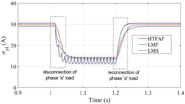
Figure 3 Comparison of HTFAF with LMS and LMF filters.
5.1 Comparative Analysis of Proposed HTFAF Filter with Exciting LMF and LMS Filter
A comparison of the estimated average active weight of load current () using HTFAF [27] with LMS [10] and LMF [11] filters is presented in Figure 3. The condition unbalanced nonlinear is considered for verifying the dynamic functioning of the filters. Phase-a of three phases balanced nonlinear load is disconnected to implement the unbalanced load on the system. As depicted in Figure 3, a balanced non-linear load is employed from 0.9 s to 1 s. At 1 s, the unbalanced non-linear load is connected. Phase-a load is again connected at 1.2 s and a balanced non-linear load is connected. It can be seen that estimated load component, , using LMS shows more chattering than LMF and HTFAF. Estimated using LMF shows less chattering than LMS. Estimated using HTFAF shows negligible chattering as compared to LMS and LMF. Furthermore, when the unbalanced non-linear load is applied, HTFAF acts faster and more accurately than LMS and LMF. Therefore, the HTFAF estimates the weights of load current active and reactive segments.
5.2 Case-I (Performance Assessment Under Unbalanced and Balanced Linear Loads)
In this case, a linear load is applied to the system and the system performance is scrutinized when it is balanced and unbalanced.
Simulated system results for this condition are presented in Figures 4 and 5. In Figure 4, gate pulses to the converter are not given at the starting, and load unbalancing is applied at 0.3 s by opening phase-a of the linear load. Once the phase ‘a’ linear load is opened at 0.3 s, the current flowing through phase-a becomes zero. As the DSTATCOM is not operated yet, phase ‘a’ grid current is zero and the other two phases are carrying currents, which are identical to the load currents between 0.3 s to 0.5 s.
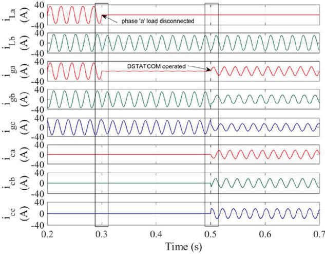
Figure 4 System performance under nonlinear unbalnced load with and without DSTATCOM operation.
The 3-phase VSC currents are zero up to 0.5 s. At 0.5 s, gate pulses to the converter are given, and the 3-phase VSC currents start to flow, which balances the grid current. Therefore, due to the implementation of the control structure, 3-phase balanced grid currents are achieved even when the applied linear load is unbalanced, which is observed in Figure 4.
In Figure 5, when a balanced linear load is connected, currents in all three phases are sinusoidal until 0.3 s, as shown. When the phase-a linear load is detached to create unbalancing at 0.3 s, the current in that phase becomes zero. Despite that, the currents in the other two phases remain to flow. From the grid currents (i), it can be perceived that the grid currents are balanced despite the load is unbalanced. The DC voltage follows the reference value perfectly, even under an unbalanced load.
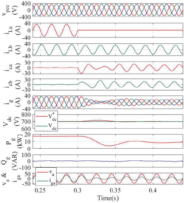
Figure 5 System performance under 3-phase linear balanced and unbalanced loads (PFC mode).
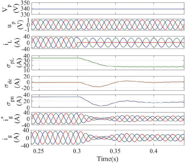
Figure 6 Reference currents determination under unbalanced and balanced linear loads.
When the phase-a linear load is detached at 0.3 s, the effective load on the system decreases, and the grid currents flow with low magnitude, which is observed from the grid currents and the grid power (P). The reactive power of the grid is nearly zero throughout the period. It verifies that the PF of the supply side is almost unity. The grid voltage is scaled down (v) and compared with the grid current (i). It shows no phase delay between the grid voltage and grid current.
Moreover, there is no variation in the PCC voltage during this variation of linear unbalance load. Simulation results showing the calculation procedure of reference grid currents are displayed in Figure 6. The magnitude of the PCC voltage is maintained. The unit templates are perfectly sinusoidal with unit values. With the detachment of phase-a linear load, the active average load weight () decreases, the DC loss component () varies to sustain the DC-link voltage and the net active component also decreases. Perfectly sinusoidal and balanced reference grid currents are determined. Furthermore, it can be perceived that the actual grid currents (i) are following the reference currents (). Estimation of load weights at linear balanced and unbalanced loads using HTFAF are displayed in Figure 7. It can be perceived that the phase-a load weight () becomes zero when the phase-a linear load is separated at 0.3 s. However, the phases ‘b’ and ‘c’ (, ) contribute to the average load weight calculation. Therefore, the average active weight of load current () is reduced upon applying an unbalanced load. Thus, simulated results confirm the satisfactory operation of the system under linear balanced as well as unbalanced loads.
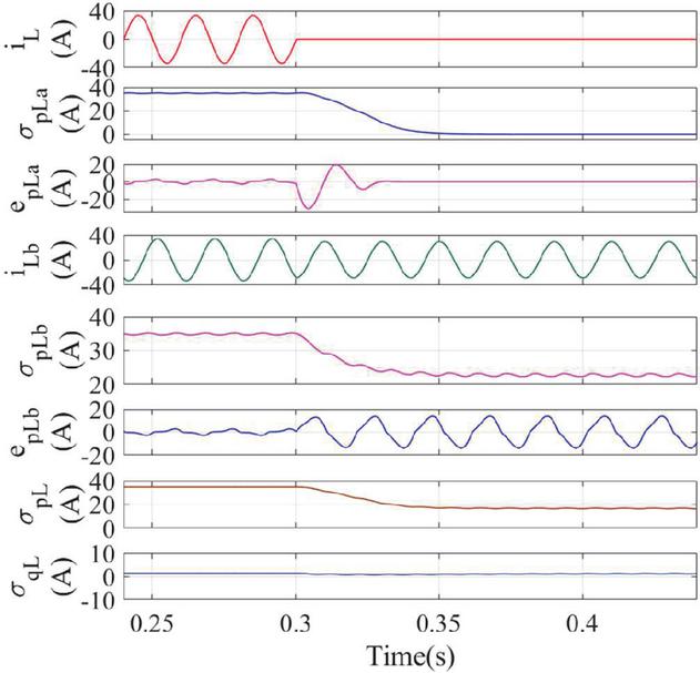
Figure 7 Estimation of weights using HTFAF for balanced and unbalanced linear loads.
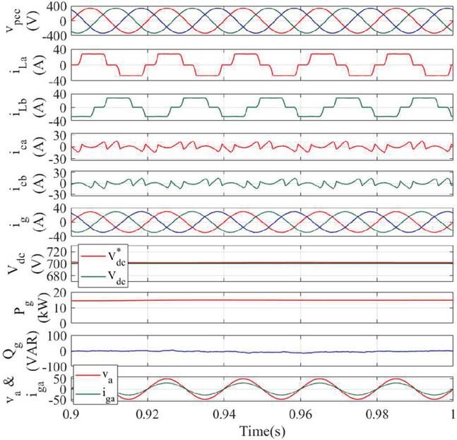
Figure 8 Performance of the system under 3-phase nonlinear balanced load (PFC mode).
5.3 Case-II (Performance Assessment Under Balanced Nonlinear Load)
A nonlinear balanced load (diode bridge rectifier (DBR) with an RL load) is applied in this case, and simulation outcomes are presented in Figure 8. From the results, it can be noticed that the load currents are of quasi square wave nature, which contains harmonics. Even if the load currents are nonlinear, the grid currents are sinusoidal, which verifies that the grid currents’ harmonics contents are negligible compared to the load currents. The load’s harmonics and reactive power requirement are supplied by the DSTATCOM as observed from the DSTATCOM currents. DC-link voltage is perfectly tracking the reference value. The reactive power is nearly zero, proving that the PF is nearly unity.
5.4 Case-III (Performance Assessment Under Unbalanced and Balanced Nonlinear Load)
At first, the system is under a 3-phase balanced nonlinear load (i.e., up to 1 s) without firing the switches of the converter. In the absence of switching pulses, the phase-a load is disconnected at 1 s, as shown in Figure 9.
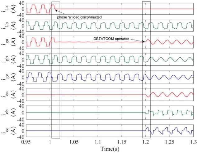
Figure 9 System performance under nonlinear unbalanced load with and without DSTATCOM operation.
In this condition, phase-a load current becomes zero, and currents flow in the other two phases. Since DSTACOM is not operated yet, the phase-a grid current is zero, and currents in the other two phases are identical. It shows that an unbalanced load draws unbalanced currents from the grid (i.e., between 1 to 1.2 s). Now, the switching pulses are sent to the converter at 1.2 s. Due to the DSTATCOM operation with the proposed control structure, sinusoidal and balanced grid currents flow in the system even though the load is unbalanced.
In Figure 10, an unbalanced nonlinear load is applied at 1 s and again, it is made balanced at 1.2 s. The results show that upon detachment of phase-a non-linear load, the current in phase-a get to be zero whereas the current is flowing in phase-b between 1 s to 1.2 s. The grid currents are noticed as balanced and sinusoidal. It is due to the supply of nonlinearity by the DSATCOM to keep the balanced grid currents. Due to the system’s reduced loading, the grid power is reduced to meet the load requirement. Moreover, the unity PF at the supply end is attained, which can be validated from zero reactive grid power, as observed in Figure 10. Simulated results for demonstrating the reference currents generation are depicted in Figure 11.
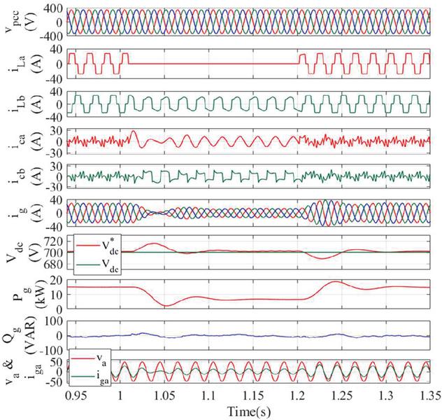
Figure 10 Performance of the system under 3-phase nonlinear unbalanced load.
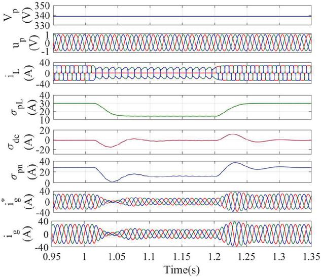
Figure 11 Reference currents determination under balanced and unbalanced nonlinear loads.
In Figure 11, the average active weight of the load is illustrated, which reduces with phase-a load disconnection. The DC loss weight is adjusted to track the reference DC link voltage. The net active weight reduces, which shows the decrement in the grid current peak. The estimation of active load weights using HTFAF is presented in Figure 12. In this figure, the performance of the implemented filter is shown, which verifies the effective operation of the filter and the system when it is applied.
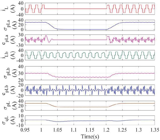
Figure 12 Estimation of weight using HTFAF for balanced and unbalanced nonlinear loads.
5.5 Case-IIV (Performance Assessment Under Voltage Sag (ZVR Mode))
A voltage sag command is applied, and the system performance is assessed. Simulated results, for this event, are depicted in Figure 13, Figures 14, and 15. In Figure 13, balanced voltage sag is applied at 0.5 s when the system is loaded by a nonlinear balanced load. ZVR mode of operation is included. Under the voltage dip in PCC, the DSTATCOM delivered the reactive power to stabilize the PCC voltage. Therefore, the DSTATCOM provides the active and reactive components of currents. Adding a reactive segment with the active segment increases the magnitude of resultant grid currents. The actual grid currents are tracking the reference currents satisfactorily. Due to the reactive power supply, a clear phase shift is noticed between the grid phase voltage and currents.
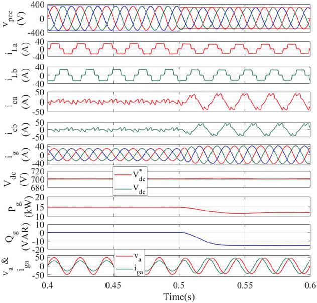
Figure 13 Performance of the system under voltage sag (ZVR Mode).
In this case, the PF is not unity. Even in this condition, the weights of the load currents are estimated perfectly using HTFAF. Simulated results of reference currents generation under voltage sag utilizing the suggested control structure are presented in Figure 14.
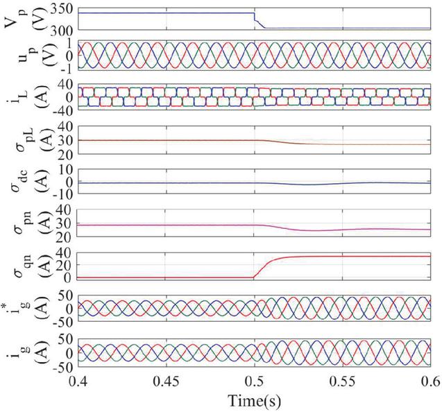
Figure 14 Determination of reference currents under voltage sag.
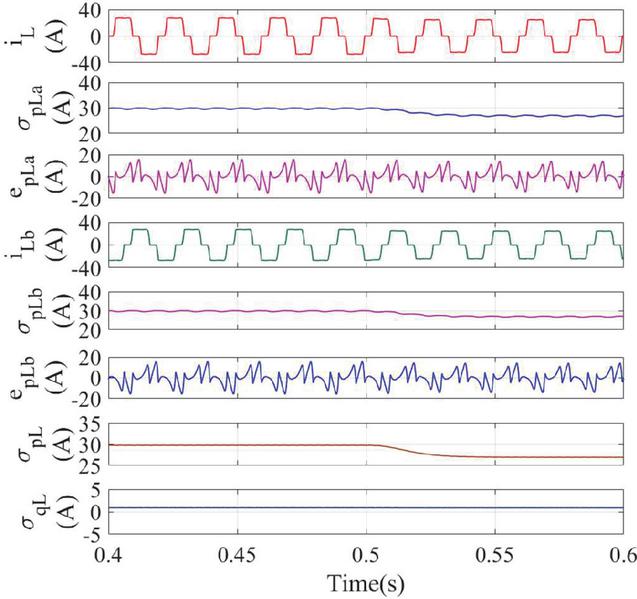
Figure 15 Estimation of weights using HTFAF for voltage sag.
The result exhibits that once the voltage sag is applied at 0.5 s, the magnitude of PCC voltage is reduced. The net reactive weight increased, which shows the increase in the grid current peak. The reference grid currents, and sensed grid currents are presented that show their expected behavior under voltage sag. Simulated results of the weights using HTFAF are shown in Figure 15 under voltage sag conditions. In Figure 15, the performance of the implemented filter is shown, which verifies the effective operation of the filter and the system when voltage sag is applied.
6 Real-Time Results
The test system shown in Figure 1 along with the control structure presented in Figure 2 is conducted in a real-time simulator (OP4510) and results are obtained in order to validate the result in actual electrical conditions. The prototype shown in Figure 16 consists of OPAL-RT (OP4510) for the test system real-time simulation, host PC to interface RT-LAB software (loaded in host PC) and DAC (Digital to Analog Card) for communication with the real time environment and DSO for capturing the real-time results. The RT-LAB is used to compile the model to executable code which is run on OPAL-RT simulator. Then, central processing unit of OPAL-RT run this executable code and produces real time result. The real time results obtained from the OPAL-RT are taken in the DSO as depicted in the Figure 16.
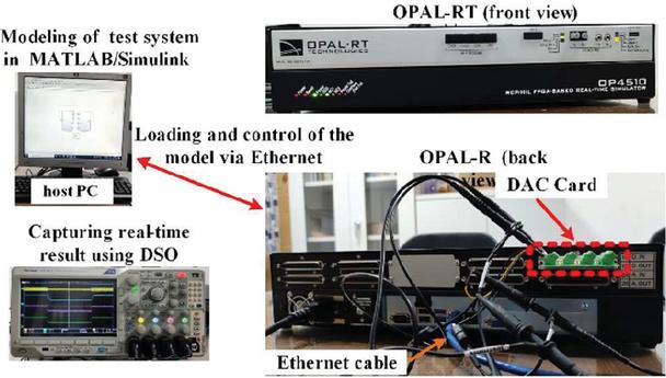
Figure 16 Prototype of the system.
The system performance is obtained for both nonlinear and linear loads with unbalanced and balanced events. Figures 17 and 18 show the system performance under linear balanced and unbalanced loads before and after applying switching pulses to the converter. It is seen that when gate pulses are not given to the converter, the grid currents are identical to the load. Hence, an unbalanced load draws unbalanced currents from the grid and the compensating currents or DSTATCOM currents from the VSC are zero. On the other hand, when the gate pulses are given to the VSC, the compensating currents start to flow, and balanced grid currents are achieved under an unbalanced linear load.
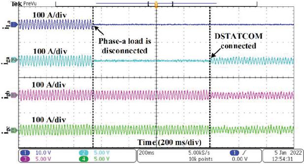
Figure 17 Real-time results showing the phase-a load current and 3-phase grid currents under linear balanced and unbalanced loads.
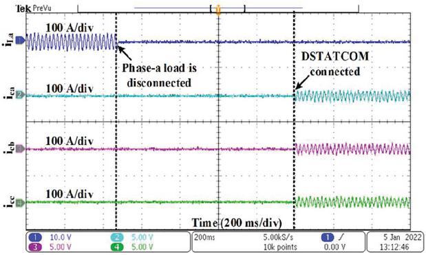
Figure 18 Real-time results showing the phase-a load current and 3-phase VSC currents under linear balanced and unbalanced loads.
Similarly, Figures 19 and 20 show the system performance under nonlinear balanced and unbalanced load before and after applying switching pulses to the converter. It is seen that before the application of gate pulses to the converter, the nonlinear unbalanced load draws nonlinear unbalanced currents from the grid. However, when the DSTATCOM is operated, nonlinear unbalanced load draws balanced and sinusoidal currents from the grid and the DSTATCOM provides the compensating currents.
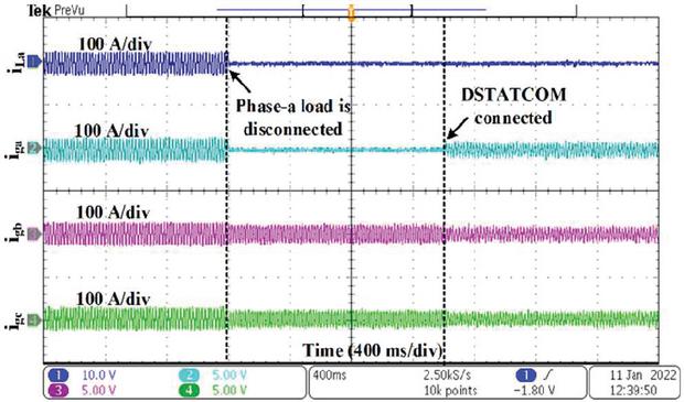
Figure 19 Real-time results showing the phase-a load current and 3-phase grid currents under nonlinear balanced and unbalanced loads.
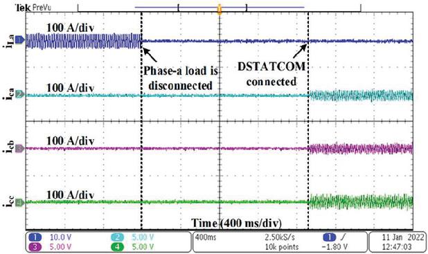
Figure 20 Real-time results showing the phase-a load current and 3-phase VSC currents under nonlinear balanced and unbalanced loads.
7 Conclusion
A hyperbolic tangent function-based adaptive filter (HTFAF) has been used for fast and accurate operation of static compensator. Extensive simulation results have been presented under two operating conditions as PFC and ZVR. The performance of the proposed control structure under PFC mode has been verified by applying linear/nonlinear balance/unbalance loads. The ZVR mode of operation has been demonstrated for the proposed control structure at balanced voltage sag and filter performance. Moreover, the control structure is also compared with exiting control structure LMF and LMS. The simulation results have been found satisfied in all the tested conditions. The grid connected static compensator and control structure has been designed using MATLAB/Simulink environment. The performance of the system is also validated using the OPAL-RT real-time simulator. From the results, it has been observed that the compensation currents have been supplied by the DSTATCOM to satisfy the nonlinearity of load and balance the grid currents.
Appendix
This declaration is not applicable.
Competing Interests
Authors declare that they have not any competing interest.
Funding
This work has not been funded by any organization.
Availability of Data and Materials
The data can be available from the authors upon reasonable request.
References
[1] Z. Salameh, “Factors Promoting Renewable Energy Applications,” Renew. Energy Syst. Des., pp. 1–32, 2014, doi: 10.1016/B978-0-12-374991-8.00001-5.
[2] B. Singh, P. Jayaprakash, D. P. Kothari, A. Chandra, and K. Al Haddad, “Comprehensive study of dstatcom configurations,” IEEE Trans. Ind. Informatics, vol. 10, no. 2, pp. 854–870, 2014, doi: 10.1109/TII.2014.2308437.
[3] A. Medina-Rios and H. A. Ramos-Carranza, “An Active Power Filter in Phase Coordinates for Harmonic Mitigation,” IEEE Trans. Power Deliv., vol. 22, no. 3, pp. 1991–1993, 2007, doi: 10.1109/TPWRD.2007.899985.
[4] M. H. J. Bollen, Understanding power quality problems: Voltage sags and interruptions. IEEE Press, 1999.
[5] M. P. Kazmierkowski, “Power Quality: Problems and Mitigation Techniques [Book News],” IEEE Industrial Electronics Magazine, vol. 9, no. 2. John Wiley & Sons, WS, UK, p. 62, 2015, doi: 10.1109/MIE.2015.2430111.
[6] S. Vanga and S. N. V. Ganesh, “Comparison of Fourier Transform and Wavelet Packet Transform for quantification of power quality,” 2012 Int. Conf. Adv. Power Convers. Energy Technol. APCET 2012, 2012, doi: 10.1109/APCET.2012.6302048.
[7] J. Ma, X. Wang, Y. Zhang, Q. Yang, and A. G. Phadke, “A novel adaptive current protection scheme for distribution systems with distributed generation,” Int. J. Electr. Power Energy Syst., vol. 43, no. 1, pp. 1460–1466, Dec. 2012, doi: 10.1016/j.ijepes.2012.07.024.
[8] M. A. Mostafa, “Kalman filtering algorithm for electric power quality analysis: Harmonics and voltage sags problems,” LESCOPE’07 – 2007 Large Eng. Syst. Conf. Power Eng., pp. 159–165, 2007, doi: 10.1109/LESCPE.2007.4437371.
[9] J. Bangarraju, V. Rajagopal, S. R. Arya, and B. Subhash, “Enhancement of PQ Using Adaptive Theorybased Improved Linear Tracer SinusoidalControl Strategy for DVR,” J. Green Eng., vol. 7, no. 1, pp. 189–212, Jan. 2017, doi: 10.13052/JGE1904-4720.7129.
[10] M. Srinivas, I. Hussain, and B. Singh, “Combined LMS-LMF-Based Control Algorithm of DSTATCOM for Power Quality Enhancement in Distribution System,” IEEE Trans. Ind. Electron., vol. 63, no. 7, pp. 4160–4169, Jul. 2016, doi: 10.1109/TIE.2016.2532278.
[11] B. Singh and S. R. Arya, “Implementation of single-phase enhanced phase-locked loop-based control algorithm for three-phase DSTATCOM,” IEEE Trans. Power Deliv., vol. 28, no. 3, pp. 1516–1524, 2013, doi: 10.1109/TPWRD.2013.2257876.
[12] S. R. Arya and B. Singh, “Performance of DSTATCOM using leaky LMS control algorithm,” IEEE J. Emerg. Sel. Top. Power Electron., vol. 1, no. 2, pp. 104–113, 2013, doi: 10.1109/JESTPE.2013.2266372.
[13] R. K. Agarwal, I. Hussain, and B. Singh, “Application of LMS-based NN structure for power quality enhancement in a distribution network under abnormal conditions,” IEEE Trans. Neural Networks Learn. Syst., vol. 29, no. 5, pp. 1598–1607, 2018, doi: 10.1109/TNNLS.2017.2677961.
[14] S. Pradhan, I. Hussain, B. Singh, and B. Ketan Panigrahi, “Performance improvement of grid-integrated solar PV system using DNLMS control algorithm,” IEEE Trans. Ind. Appl., vol. 55, no. 1, pp. 78–91, 2019, doi: 10.1109/TIA.2018.2863652.
[15] A. Bag, B. Subudhi, and P. Ray, “An Adaptive Variable Leaky Least Mean Square Control Scheme for Grid Integration of a PV System,” IEEE Trans. Sustain. Energy, vol. 11, no. 3, pp. 1508–1515, 2020, doi: 10.1109/TSTE.2019.2929551.
[16] D. J. Hogan, F. J. Gonzalez-Espin, J. G. Hayes, G. Lightbody, and R. Foley, “An adaptive digital-control scheme for improved active power filtering under distorted grid conditions,” IEEE Trans. Ind. Electron., vol. 65, no. 2, pp. 988–999, 2017, doi: 10.1109/TIE.2017.2726992.
[17] Z. Xin, X. Wang, Z. Qin, M. Lu, P. C. Loh, and F. Blaabjerg, “An Improved Second-Order Generalized Integrator Based Quadrature Signal Generator,” IEEE Trans. Power Electron., vol. 31, no. 12, pp. 8068–8073, 2016, doi: 10.1109/TPEL.2016.2576644.
[18] G. S. Chawda and A. G. Shaik, “Enhancement of Wind Energy Penetration Levels in Rural Grid Using ADALINE-LMS Controlled Distribution Static Compensator, ” IEEE Transactions on Sustainable Energy, vol. 13, no. 1, pp. 135–145, Jan. 2022. doi: 10.1109/TSTE.2021.3105423.
[19] C. Balasundar, C. K. Sundarabalan, S. N. Santhanam, J. Sharma and J. M. Guerrero, “Mixed Step Size Normalized Least Mean Fourth Algorithm of DSTATCOM Integrated Electric Vehicle Charging Station,” IEEE Transactions on Industrial Informatics, 2022. doi: 10.1109/TII.2022.3211958.
[20] A. Dash, U. R. Muduli, S. Prakash, K. A. Hosani, S. R. Gongada and R. K. Behera, “Modified Proportionate Affine Projection Algorithm Based Adaptive DSTATCOM Control With Increased Convergence Speed, ” IEEE Access, vol. 10, pp. 43081–43092, 2022. doi: 10.1109/ACCESS.2022.3169618.
[21] S. Kumar, D. Jaraniya, R. R. Chilipi and A. Al-Durra, "Optimal Operation of WL-RC-QLMS and Luenberger Observer Based Disturbance Rejection Controlled Grid Integrated PV-DSTATCOM System”, IEEE Transactions on Industry Applications, vol. 58, no. 6, pp. 7870–7880, Nov.–Dec. 2022. doi: 10.1109/TIA.2022.3199401.
[22] S. K. Sahoo, S. Kumar and B. Singh, “Wiener Variable Step Size With Variance Smoothening Based Adaptive Neurons Technique for Utility Integrated PV-DSTATCOM System, ” in IEEE Transactions on Industrial Electronics, vol. 69, no. 12, pp. 13384–13393, Dec. 2022. doi: 10.1109/TIE.2021.3134077.
[23] C. Zhang, X. Zhao, X. Wang, X. Chai, Z. Zhang, and S. Member, “A Grid Synchronization PLL Method Based on Mixed Second- and Third-Order Generalized Integrator for DC Offset Elimination and Frequency Adaptability,” vol. 6, no. 3, pp. 1517–1526, 2018, doi: 10.1109/JESTPE.2018.2810499.
[24] C. M. Hackl, S. Member, and M. Landerer, “Modified Second-Order Generalized Integrators With Modified Frequency Locked Loop for Fast Harmonics Estimation of Distorted Single-Phase Signals,” IEEE Trans. Power Electron., vol. 35, no. 3, pp. 3298–3309, 2020, doi: 10.1109/TPEL.2019.2932790.
[25] R. Panigrahi, P. C. Panda, and B. Subudhi, “A Robust Extended Complex Kalman Filter and Sliding-mode Control Based Shunt Active Power Filter,” Electr. Power Components Syst., pp. 520–532, 2014, doi: 10.1080/15325008.2013.871609.
[26] X. Guo and J. M. Guerrero, “Abc-frame complex-coefficient filter and controller based current harmonic elimination strategy for three-phase grid connected inverter,” J. Mod. Power Syst. Clean Energy, vol. 4, no. 1, pp. 87–93, 2016, doi: 10.1007/s40565-016-0189-4.
[27] I K. Kumar, S. S. Bhattacharjee, and N. V George, “Joint Logarithmic Hyperbolic Cosine Robust Sparse Adaptive Algorithms,” vol. 68, no. 1, pp. 526–530, 2021, doi:10.1109/TCSII.2020.3007798.
[28] IEEE, “IEEE Std 519-2014: IEEE Recommended Practice and Requirements for Harmonic Control,” ANSI/IEEE Std. 519, vol. 2014, pp. 5–9, 2014.
[29] H. Akagi, E. H. Watanabe, and M. Aredes, Instantaneous Power Theory and Applications to Power Conditioning, 2nd ed. Hoboken, New Jersey, US: John Wiley & Sons, Inc., 2017.
Biographies

Jeetendra Kumar received his BE degree in Electrical & Electronics Engineering from Anna University, Chennai, Tamil Nadu, India, in 2011 and his MTech degree in Control & Instrumentation from Motilal Nehru National Institute of Technology, Allahabad, Uttar Pradesh, India, in 2016. Presently, he is pursuing a PhD at the Department of Electrical Engineering, NIT Jamshedpur, Jharkhand, India. He is an Assistant Professor in the Department of Electrical Engineering at the Government Engineering College, Bhojpur, India. His areas of interest are renewable energy and power quality enhancement.

Salauddin Ansari received his BE degree in Electrical & Electronics Engineering from Rajiv Gandhi Proudyogiki Vishwavidyalaya, Bhopal, Madhya Pradesh, India, in 2015, and his MTech and PhD degrees from the National Institute of Technology, Jamshedpur, Jharkhand, India, in 2019 and 2024, respectively. He heads the Electrical Engineering Department at Government Polytechnic, Motihari, Bihar, India. His primary research interests include microgrid protection and islanding detection.

Om Hari Gupta earned his PhD in Electrical Engineering from the IIT Roorkee, India, in 2017. He was awarded the prestigious Canadian Queen Elizabeth II Diamond Jubilee Scholarship, enabling him to conduct research at Ontario Tech University, Canada, as a visiting researcher in 2017. Since 2018, Dr. Gupta has been an Assistant Professor in the Department of Electrical Engineering at NIT Jamshedpur, India. Dr. Gupta co-founded the “Electric Power and Renewable Energy Conference (EPREC)” series and has authored/edited seven books. His academic contributions include about 90 publications, with 34 journal papers and one granted patent. He serves on the Springer Nature Journal Scientific Reports editorial board and is a Senior Member of IEEE. Additionally, he is a reviewer for numerous reputed journals, including IEEE Transactions on Power Delivery, Electric Power Systems Research, etc. His research interests encompass power system protection, microgrids, renewable energy-based distributed generation, and electric power quality.

Arun Kumar Singh has served as a Professor at the Department of Electrical Engineering, National Institute of Technology Jamshedpur, India. He received his B.Sc. (Engg.) from Kurukshetra University, Kurukshetra; M. Tech from the Banaras Hindu University, Varanasi; and PhD in electrical engineering from the Indian Institute of Technology Kharagpur, India. He has over 30 years of teaching experience and has taught subjects like Control Systems, Control & Instrumentation, Power System Operation and Control, Non-Conventional Energy, and Circuit & Network Theory. His primary research interests include control systems, control system applications in different areas & non-conventional energy. Prof. Singh is a Life Member of ISTE and a life fellow of the Institute of Engineers. He has been the Dean of Student Welfare at the National Institute of Technology.

Vijay K. Sood obtained his Ph.D. in Power Electronics from the University of Bradford, England in 1977. From 1969–76, he was employed at the Railway Technical Centre, Derby, U.K. From 1976–2007, he was a Senior Researcher at IREQ (Hydro-Québec Research Institute) in Montreal, Quebec. In 2007, he joined Ontario Tech University in Oshawa, Ontario where he is now Professor Emeritus. He is a Member of the Professional Engineers Ontario, a Life Fellow of the Institute of Electrical and Electronic Engineers (IEEE), a Fellow of the Engineering Institute of Canada (EIC) and Emeritus Fellow of the Canadian Academy of Engineering (CAE). His research interests are in the monitoring, control and protection of power systems using artificial intelligence techniques. Dr. Sood has published over 200 articles, 10 book chapters and written numerous books on HVDC Transmission and other topics.
Distributed Generation & Alternative Energy Journal, Vol. 40_1, 29–62.
doi: 10.13052/dgaej2156-3306.4012
© 2025 River Publishers