A Two-stage Optimal Dispatching Method of Distribution Network Considering the High Proportion of Distributed Renewable Energy Penetration
JinSen Liu1,*, Ning Luo1, LuDong Chen1, Fei Zheng1 and Chang Xu2
1Power Grid Planning and Research Center of Guizhou Power Grid Co., Ltd., Guiyang, 550003, GuiZhou, China
2Guizhou Power Grid Co., Ltd., Guiyang, 550000, GuiZhou, China
E-mail: bywdlwaucc@163.com
*Corresponding Author
Received 26 December 2024; Accepted 07 March 2025
Abstract
The increased incorporation of distributed renewable energy (DRE) into distribution networks has presented new obstacles to the planning and operation of these systems due to its intermittency and volatility. This research examines the integration of DRE by modeling the output characteristics of distributed energy and the load fluctuation characteristics of the distribution network with deep learning technology. Specifically, the Long Short-Term Memory (LSTM) model is adopted to create a dynamic output prediction model, which is used to analyze the impact mechanism of the dual volatility of “source and load” on distribution network planning with the incorporation of DRE. Thus, a dual-phase optimization approach for day-ahead and intra-day planning is suggested to improve distribution network decisions from both safety and economic perspectives. The aim is to improve the system’s capacity for renewable energy utilization, financial benefits, and operational reliability. Additionally, a real-time optimization method and a model validation framework are developed.
Keywords: DRE, distribution network, output prediction, optimization method.
1 Introduction
China has to accelerate the transformation of energy production and consumption, support the development of new energy installations, and ease the transfer to low-carbon power producing companies in order to achieve carbon peaking and carbon neutrality. According to data published by the National Energy Administration in 2024, the total installed capacity of wind power in the country has grown to around 440 GW, representing a notable 20.7% annual increase [1].
Large-scale wind power curtailment is still a major problem in some areas of China, despite the country’s wind power installations growing quickly. The worst-affected area, eastern Inner Mongolia, had a wind power utilization rate of only 90% in 2022, which was far lower than the 96.8% national average [2]. One of the biggest obstacles to China’s energy development is addressing the problem of massive wind power consumption.
The large-scale integration of DRE into distribution networks has introduced dual uncertainties in “source-load” dynamics, affecting the safe and stable supply of electricity and the market-based consumption of DRE. Meanwhile, high-energy-consuming loads typically exhibit characteristics such as rapid response capabilities, large adjustment capacities, and good operational stability [3]. In the context of large-scale DRE integration encountering curtailment in distribution networks, high-energy-consuming loads can promptly adjust to changes in wind power, therefore locally utilizing the restricted wind energy and enhancing wind power utilization rates.
Therefore, under the premise of increasing wind power capacity and expanding high-energy-consuming enterprises, conducting feasibility and quantitative studies on load-side resource participation in distributed wind power peak shaving can effectively achieve the complementary and coordinated development of distributed wind power and high-energy-consuming enterprises in distribution networks [4].
At present, relevant studies have been conducted both domestically and internationally to address the issue of large-scale wind power curtailment by incorporating load-side resources and thermal power units into distribution network optimization scheduling [5–7]. Reference [8] presents price-based and incentive-based demand response, developing an optimization scheduling model for wind power utilization that incorporates several demand response types, and validates the model’s efficacy through case studies. References [9, 10] consider both the demand side and supply side, involving adjustable loads and conventional power sources in coordinated grid optimization scheduling, thereby forming a source-load coordinated operation mode to improve wind power consumption levels and economic efficiency. Reference [11] achieves effective coordination of various demand-side resources through optimized power system scheduling, enabling regulation resources with different response speeds to function optimally within their respective time scales, significantly improving scheduling efficiency and response capabilities. Reference [12] introduces a novel method of integrating electrochemical energy storage into a heat storage electric boiler system, achieving effective synergy between energy storage technology and heat storage boilers, thereby consuming wind power while enhancing grid stability. This method opens new avenues for addressing renewable energy consumption challenges and brings innovative ideas and possibilities for energy transition and power system optimization.
Reference [13] suggests a demand-responsive multi-stage scheduling strategy for studies on employing high-energy-consuming loads to help overcome DRE consumption issues. In order to resolve the mismatch between the regulation characteristics of high-energy-consuming loads and wind power output characteristics, this model thoroughly examines ways for various high-energy-consuming load types to participate in demand response. This allows wind power and multiple high-energy-consuming load types to operate together. In order to effectively manage power allocation and trading between high-energy-consuming loads and wind power, Reference [14] thoroughly examines power coordination and trading models between renewable energy and high-energy-consuming loads. It then suggests a coordinated scheduling strategy based on the fundamental idea of energy internet users. By suggesting a novel load-source control technique based on the operating characteristics of high-energy-consuming loads, Reference [15] tackles wind power curtailment difficulties. By rolling optimization of energy and power across several time scales, this technique maximizes wind power consumption while achieving coordinated control of demand and supply. A multi-objective optimization scheduling method is proposed in Reference [16], which investigates the effects of source-load coordination on wind power consumption and economic operation. An efficient guide for creating wind power consumption scheduling strategies is provided by the fuzzy membership function, which is utilized to determine the ideal solution for the multi-objective model, which is designed to optimize wind power consumption and reduce system operation costs.
The aforementioned studies emphasize the optimization of system resources while focusing on wind power consumption through the lens of source-load coordination. However, there are a number of shortcomings in the research, such as a failure to pay enough attention to time scales and a failure to consider the regulatory differences among various types of high-energy-consuming loads over various time horizons.
In order to improve wind power forecasting accuracy as the temporal scale shrinks, this study uses the Long Short-Term Memory (LSTM) model to define the “source-load” characteristics of renewable energy and demand inside the distribution network. The feasibility of their participation in reducing wind power curtailment is investigated, and several types of high-energy-consuming loads are identified and modeled based on their modifiable characteristics.
Second, a day-ahead and intra-day two-stage wind power consumption model that involves high-energy-consuming loads is constructed. This model is established by taking into full consideration the applicability of shiftable, interruptible, and power-variable high-energy-consuming loads for various time scales.
A number of different kinds of high-energy-consuming loads and the operational restrictions of generation entities are taken into consideration when developing the model in order to achieve the goal of minimizing the total cost of the system. Ultimately, simulation analysis is performed via case studies to validate the suggested model, illustrating its crucial function in enhancing DRE consumption and ensuring the sustainable and healthy advancement of the distribution network.
2 LSTM-Based “Source-Load” Output Fluctuation Prediction Model
The extensive implementation of renewable energy has rendered precise output forecasting for wind and photovoltaic (PV) production systems a crucial technology for energy scheduling and optimization. Owing to the significant unpredictability of meteorological variables like wind velocity and solar irradiation, conventional forecasting techniques frequently fall short of achieving the necessary precision. Consequently, deep learning techniques, especially those utilizing neural network architectures, have proven to be viable solutions for tackling these difficulties. This research utilizes the LSTM network to forecast the output of DRE devices. LSTM, a specific variant of Recurrent Neural Network (RNN), proficiently captures long-term dependencies in time series data. This renders it especially appropriate for predicting output data with significant temporal correlations, such as wind power and photovoltaic energy.
2.1 Long Short-Term Memory Model
The forget gate, input gate, and output gate are the three gating mechanisms that make up the LSTM model. The current input data and the hidden state from the previous time step are sent to each gate as inputs. The LSTM can efficiently capture the temporal characteristics of wind power and solar output data thanks to these gates, which enable it to selectively update or delete information.
Define the historical output dataset of wind power or solar generation as , where denotes the output value at time step . The operational concepts of the LSTM model can be articulated by the subsequent mathematical equations.
(1) Forget Gate
The amount of data from the previous cell state that needs to be discarded is controlled by the forget gate . The forget gate’s output is a number between 0 and 1, which represents the degree of forgetfulness:
| (1) |
Here, represents the activation function of the sigmoid, and represent the forget gate’s weights and bias, respectively, while shows that the current input and the previous hidden state have been concatenated.
(2) Input Gate
How much of the current input data is used to update the cell state is determined by the input gate :
| (2) |
This formula uses the sigmoid function to control the strength of information updating.
(3) Candidate Memory Cell
The candidate memory cell is employed to create fresh memory and determine what data should be added to the cell state :
| (3) |
This formula employs the tanh activation function to transform the current input data into a new candidate memory state.
(4) Cell State
The cell state is fundamental to the LSTM, transmitting long-term dependence information from the past to the present. The input gate’s and forget gate’s complementary functions enable the cell state update:
| (4) |
In this context, and govern the weights of historical and current information within the cell state.
(5) Output Gate
At the current time step, the hidden state is defined by the output gate :
| (5) |
The hidden state at the present time step is computed using the subsequent formula:
| (6) |
The concealed state , produced by the LSTM, may be utilized for computations in the subsequent time step or for the ultimate prediction task.
3 Modeling of High-Energy-Consumption Load Characteristics in Distribution Networks
In forecasting wind power and PV output, LSTM can identify intricate patterns in time-series data. Meteorological data, including wind speed and sun irradiation, in conjunction with historical output data, serve as inputs to the LSTM. During the training phase, the model acquires the ability to forecast future outputs based on historical output patterns.
Assume our objective is to forecast the wind power or PV production at the subsequent time step . The model’s input could include meteorological data (e.g., wind velocity, solar irradiance, temperature) and historical output data spanning the present and preceding time steps. Upon training the LSTM network, it acquires the time-series characteristics pertinent to the system and produces the forecasted output:
| (7) |
In this context, represents the anticipated value at a subsequent time, while is the regression layer that converts the hidden state into the definitive prediction output.
3.1 Model Training and Optimization
The LSTM model’s training method involves minimizing prediction error. The Backpropagation Through Time (BPTT) technique is used to optimize parameters for a time series dataset of wind power or solar output . The prevalent loss function is the Mean Squared Error (MSE), defined as:
| (8) |
Here, stands for the model’s anticipated value, for the wind power or photovoltaics’ actual output value, and T for the samples.
By refining the weights and biases of the LSTM, the model can progressively enhance its predictive accuracy. Upon completion of training, the LSTM model is capable of executing real-time predictions of wind and photovoltaic output, hence facilitating optimization of power system dispatch and informed decision-making.
4 Modeling of High-Energy-Consumption Load Characteristics in Distribution Networks
4.1 Classification of High-Energy-Consumption Loads
High-energy-consumption loads (HECL) exhibit substantial regulatory capacity and robust adjustment capabilities, together with attributes such as interruptibility, transferability, and grouped switching. When substantial wind power generation varies, modifications can be implemented utilizing high-energy-demand loads. By synchronizing and optimizing HECL with traditional power sources, the variability in wind power output may be efficiently controlled [17]. Transferable loads, interruptible loads, and variable power loads are examples of HECL that are included in system regulation. Since they all belong to different high-energy-consumption categories, transferable and interruptible loads are essentially the same.
(1) Transferable Loads
Transferable loads can regulate the startup and shutdown sequence of production lines in accordance with directives from the dispatching authority. The power system must sustain equilibrium between demand and generation to provide supply stability and reliability. Transferable loads facilitate load transfer by modifying generator output or reallocating load to adapt to fluctuations in the power grid. Their operational duration can be altered flexibly, interruptions are permissible, and the total operating time is not predetermined; nonetheless, the cumulative operational time must remain constant. Given the transferable time interval , the corresponding operational characteristic diagram is as follows:
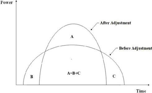
Figure 1 Power transferable load operating characteristic diagram.
The corresponding mathematical model is:
| (9) |
In the equation, indicates the load being scheduled by the system at time t, xi(t) is the variable for the adjustment state, where xi(t) 0 signifies non-participation in system regulation, and xi(t) 1 denotes participation in regulation. At time t, represents the load power of the i-th load unit involved in system scheduling.
(2) Interruptible Loads
Interruptible loads denote electrical loads within the power system that possess flexibility and adjustability, enabling them to be temporarily curtailed or diminished in response to system demands or fluctuating operating conditions. Generally, interruptible loads are managed by commercial and industrial customers who may have entered into specific agreements with power system operators. These agreements provide the decrease or cessation of power use during times of excessive system demand or emergencies, thereby mitigating system load stress and ensuring grid stability.
This adaptability allows power system operators to more efficiently manage the supply-demand equilibrium and execute control actions as necessary to maintain stable grid operations. The diagram of operational characteristics is as follows:
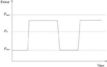
Figure 2 Interruptible load operation characteristic diagram.
The corresponding mathematical model is:
| (10) |
represents the cumulative modification of the high-energy-consumption interruptible load at time t. denotes the total count of interruptible HECL, xi(t) signifies the switching state variable of the i-th interruptible high-energy-consumption load, and shows the i-th interruptible high-energy-consumption load’s switching load magnitude at time t.
(3) Variable Power Loads
Variable power loads denote electrical loads whose power consumption is not fixed but can be modified and varied as required. These loads can attain continuous power regulation by modifying operational parameters or control systems to align with system operational requirements or dispatch directives, hence managing load variations and system alterations. In contrast to fixed loads, variable power loads provide more flexibility. Moreover, variable power loads can enhance flexibility and services by engaging in the energy market or entering agreements with power system operators, so aiding grid operation and stability.
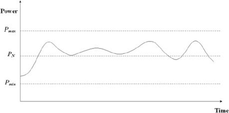
Figure 3 Power variable load operation characteristics.
Figure 3 demonstrates that when wind power output varies, HECL can promptly and consistently adjust to mitigate these changes, rendering them appropriate for intra-day optimization dispatch. The relevant mathematical model is:
| (11) |
In the equation: denotes the cumulative adjustment quantity of variable HECL at time t; represents the aggregate quantity of variable HECL; represents the switching state variable of the j-th high-energy consumption load. denotes the switching quantity of the j-th variable high-energy consumption load at time t.
4.2 Principle of Coordinated Consumption of High-Energy-Consumption Loads and DRE
Wind power generation demonstrates variability, unpredictability, and challenges in peak regulation. As the scale of wind power increases, the fluctuation of its output also intensifies, sometimes ranging from near-zero production to full rated capacity. Substantial fluctuations in wind power output increase the regulatory requirements for thermal power units. When the regulatory capacity of thermal power units is inadequate to address wind power variability, HECL may be adjusted to conform to real-time supply-demand balance needs [18].
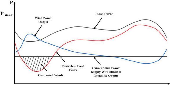
Figure 4 Schematic showing high-load capacity absorbing obstructed wind power.
Figure 4 illustrates the mechanism by which high-energy-consuming loads absorb the wind power that cannot be fully integrated. The shaded area represents the curtailed wind power under the traditional dispatching mode (Equation (13)). When high-energy-consuming loads participate in regulation, their regulation power PHECL(t) (such as the power reduction of interruptible loads or the power increase of variable loads) can fill the gap between the wind power output and the load demand (Equation (15)), thereby reducing the curtailed wind power. For example, when the wind power output surges suddenly, the system can absorb the excess wind power locally by increasing the electricity demand of variable power loads (Figure 3) or adjusting the operation period of shiftable loads (Figure 1).
The corresponding load in the conventional dispatch mode is:
| (12) |
In the equation, denotes the active load of high-energy-consumption devices in the system that do not engage in regulation, whereas represents the output of load. denotes the output of wind power.
When traditional peak-shaving resources fail to mitigate wind power oscillations, as illustrated in the shaded region of the image, wind power is curtailed, and the curtailed energy is:
| (13) |
In the equation, denotes the active load of high-energy-consumption devices in the system that do not engage in regulation.
When traditional peak-shaving resources fail to mitigate wind power oscillations, as illustrated in the shaded region of the image, wind power is curtailed, and the curtailed energy is:
| (14) |
After HECL participate in regulation, the curtailed wind power energy is
| (15) |
It can be seen that . The upward adjustment capability of HECL can follow the output of DRE to achieve consumption in situations where the grid’s peak-shaving capacity is insufficient.
Different categories of HECL exhibit variances in their involvement in regulatory approaches, necessitating a comprehensive investigation based on their operating characteristics.
4.3 Day-Ahead and Intra-Day Two-Stage Optimization Coordination Mechanism for DRE and High-Energy-Consumption Loads in Distribution Networks
Wind power capacity has grown due to the carbon peak strategy and new energy generation technology. However, wind power integration into the grid faces increasing challenges, and standard scheduling methods cannot guarantee system safety and cost efficiency [19]. For day-ahead and intra-day planning, the two-stage optimization scheduling approach uses information from many time scales to overcome renewable energy production uncertainty and unpredictability. Managing and improving grid operations enhances adaptability. Figure 5 shows the two-stage optimization scheduling model for day-ahead and intra-day operations using HECL in the distribution network.
With an hourly scheduling interval, the day-ahead scheduling plan operates on a 24-hour cycle. Taking into consideration the limitations of all power-producing organizations, the 24-hour scheduling plan is created using day-ahead wind power and load forecasts. Thermal power units take a significant amount of time to start or stop operating, thus the day-ahead plan has to specify their operational state beforehand. Additionally, the day-ahead scheduling plan must determine the dispatch quantity of shiftable and interruptible HECL for intra-day operations because they cannot be reliably changed over short time periods.
A 4-hour scheduling plan is improved at each iteration by the intra-day scheduling plan, which operates with a 15-minute scheduling interval. Intra-day optimization scheduling determines the dispatch quantities of power-adjustable, HECL, which may be continuously modified over brief periods of time, to compensate for reduced wind output brought on by inaccurate forecasts in the day-ahead plan. At the same time, the intra-day optimization scheduling uses 15-minute wind power predictions for the day to generate output plans for traditional thermal power units.
When it comes to day-ahead and intra-day operations, the two-stage optimization scheduling strategy that was discussed before is the one that optimizes the benefits of various HECL processes. In order to facilitate the adjustment of varied HECL to scheduling plans across a variety of time scales, this approach makes use of the negative correlation that exists between the accuracy of wind power output forecasts and time scale. The precision of scheduling plans is improved as a result of this, wind power variability is reduced, the usage of wind power within the system is encouraged, and overall system expenditures are reduced.
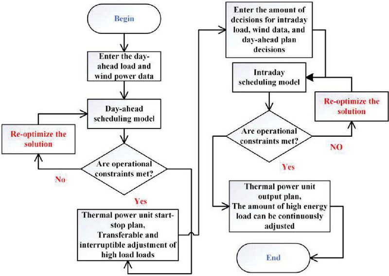
Figure 5 Flowchart of the optimization scheduling process.
5 Day-Ahead and Intra-Day Two-Stage Optimization Scheduling Model
The day-ahead and intra-day optimization scheduling models have been constructed by making use of the two-stage optimization scheduling strategy that was previously discussed for HECL. The day-ahead scheduling specifies the start/stop condition of the unit as well as the quantity of interruptible and shiftable HECL that will be dispatched for intra-day scheduling. Within the day, the intra-day scheduling makes adjustments to the power-variable, HECL dispatch in order to match with fluctuations in wind power output, which ultimately results in the most efficient application of wind energy.
5.1 Day-Ahead Optimization Scheduling Model
5.1.1 Objective function of the day-ahead optimization scheduling
The day-ahead scheduling plan functions with a 1-hour time interval across a 24-hour cycle. It thoroughly evaluates the operational limitations of diverse power producing entities and the short-term power forecasting outcomes for wind energy and load. In this way, it determines the start/stop status and output reference for conventional thermal power units for the next day and creates the electricity consumption schedule for high-energy-demanding, interruptible, and shiftable loads throughout the intra-day period. By include wind curtailment as a cost element in the total system expense, the day-ahead scheduling plan aims to reduce the system cost as a whole. The exact model looks like this:
| (16) | |
| (17) | |
| (18) | |
| (19) | |
| (20) | |
| (21) | |
| (22) |
In Equations (16)–(22), the following variables are defined: : Operating cost of thermal power units; : Cost of starting and stopping thermal power units; : Wind curtailment penalty cost for the system; ; ; : The unit dispatch cost for interruptible, shiftable, and power-variable HECL, respectively; : The quantity of thermal power units; : The thermal power units’ output over time t; The unit wind curtailment penalty cost for wind farms; : The anticipated wind turbine power production at that moment t; : the wind turbines’ real power production at any given moment t; : The number of periods with wind curtailment.
These elements are used to build the optimization model, which aims to control wind curtailment, thermal power unit operation, and HECL allocation while optimizing the overall system cost. This ensures cost reduction, grid operating efficiency, and the best possible integration of renewable energy.
5.2 Day-Ahead Optimization Scheduling Constraints
5.2.1 System power balance constraint
At each given time t, the system power balancing constraint makes sure that the total power generation from all sources equals the total power consumption. This restriction is stated as:
| (23) |
Where: denotes the output power of thermal power units at time t; denotes the wind power generated at time t; is the active power prediction for the conventional load at time t; is the dispatch power of interruptible HECL at time t post-optimization; is the shiftable HECL’s dispatch power at time t following optimization; is the power-variable HECL’s dispatch power at time t following optimization.
5.2.2 Spinning reserve constraint
Wind power installations, while generating energy, must retain a specific reserve capacity to accommodate abrupt load variations or equipment malfunctions. To guarantee the power system can swiftly adapt and sustain stable operation during unforeseen fluctuations in wind power output, limitations on both positive and negative spinning reserve capacity are implemented. These constraints guarantee the proposed model’s efficacy in real applications.
| (24) | |
| (25) |
In the equations, and are the thermal power units’ maximum and minimum output powers, respectively; and are the positive spinning reserve for load and wind power output forecast errors, respectively, at time ; and are the negative spinning reserve for load and wind power output forecast errors, respectively, at time .
5.2.3 Wind power output constraints
| (26) |
Where is the wind farm’s anticipated active electricity output at that moment.
5.2.4 Thermal power unit operating condition constraints
Constraints on the Initiation and Termination of Thermal Power Units:
| (27) |
This limitation restricts the frequency of start-up and shut-down activities of the thermal power units during the schedule period.
| (28) |
Constraints on the ramp rate of thermal power units:
| (29) | |
| (30) |
In Equations (28)–(30), The unit’s operating state variable at time t is denoted by , where 0 denotes that the device is turned off and 1 denotes that it is operating; The unit’s maximum permitted number of start-up and shutdown operations within the scheduling period is denoted by Mk; At time t, represents the thermal power unit’s output power; is the thermal power unit’s upward ramp rate; is the thermal power unit’s downward ramp rate.
5.2.5 Interruptible high-energy-consumption load scheduling constraints
Operating power upper and lower limit constraints:
| (31) |
In the equation, and are the lower and upper limits of the interruptible high-energy-consumption load power, respectively.
Regulation power upper and lower limit constraints:
| (32) |
In the equation, and are the adjustable power’s upper and lower bounds for the i-th interruptible high-energy-consumption load per unit of time, respectively.
Regulation duration constraint:
| (33) |
In the equation, is the regulation duration for the i-th interruptible high-energy-consumption load, while and are the shortest and longest durations for the i-th interruptible high-energy-consumption load’s participation in system regulation, respectively.
Regulation frequency constraint:
| (34) |
In the formula, is the maximum allowed regulation frequency for the interruptible high-energy-consumption load.
5.2.6 Transferable high-energy-consumption load scheduling constraints
Power upper and lower limit constraints:
| (35) |
Continuous operation time constraint:
| (36) |
5.2.7 Power-variable high-energy-consumption load scheduling constraints operating power upper and lower limit constraints
| (37) |
In the formula, and are the lower and upper limits of the power for the power-variable high-energy-consumption load, respectively.
Response speed constraint:
| (38) |
In the equation, and are the ramp speeds that go up and down for the i-th power-variable high-energy-consumption load, respectively.
5.3 Intra-day Optimization Scheduling Model
5.3.1 Intra-day optimization scheduling objective function
Using decision variables for thermal power units determined by day-ahead scheduling and ultra-short-term wind power output projections, intra-day scheduling aims to maximize power system coordination and optimization. The goal is to maintain the steady operation of the electrical system while striking a balance between supply and demand. Optimizing the overall cost of the system is the goal function for intra-day scheduling. The switching costs for these loads and the start-stop costs for thermal power units are considered fixed values and are not included in the formula since the call quantities for interruptible and transferable HECL and the start-stop schedules for thermal power units are preset in the day-ahead scheduling. The following is an outline of the exact intra-day optimization scheduling model:
| (39) | |
| (40) | |
| (41) | |
| (42) |
5.3.2 Intra-day optimization scheduling constraints
System power balance constraint:
| (43) |
The day-ahead scheduling has the same limitations for wind power production, spinning reserve, thermal power unit operating conditions, and power-variable high-energy-consumption load scheduling.
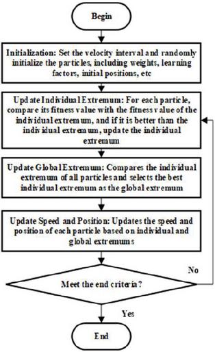
Figure 6 Flow chart of particle swarm optimization.
5.3.3 Model optimization solution method
In a multi-agent optimization system (MAOS), the particles of the Particle Swarm Optimization (PSO) algorithm possess individual memory during the search phase, enabling them to update their velocity and position via an information-sharing mechanism within the population. This information-sharing technique enables the particles to progress toward a more optimal route, hence expediting the algorithm’s convergence. The Particle Swarm Optimization algorithm comprises four primary steps: startup, evaluation, updating, and searching. The full procedure is illustrated in the diagram.
The velocity update formula and position update formula for the particle are as follows:
| (44) | |
| (45) |
Where and depict the particle’s location and velocity vectors in the d-th dimension at the k-th iteration, respectively. The impact of the velocity of the previous generation on the velocity of the present generation is indicated by the inertia weight . The particle explores new search regions faster when is greater, helping the algorithm search for the global optimum. However, too large an inertia weight may cause the algorithm to prematurely converge to a local optimum, ignoring other potentially better solutions across the global search space.
The aspect of individual learning and the social (group) learning factor affect the particle’s step size toward its own historical best position and the group’s historical best position, respectively. The individual learning factor reflects the particle’s reliance on its own experience, while the social learning factor reflects the particle’s dependence on shared information within the group.
and are arbitrary values between 0 and 1 that add unpredictability to the search procedure. symbolizes the particle’s historical best location in the d-th dimension at the k-th iteration, and symbolizes the group’s historical peak position in the d-th dimension at the k-th iteration.
The conventional Particle Swarm Optimization (PSO) algorithm, while possessing benefits such as rapid convergence and straightforward computing procedures, also encounters challenges including diminished computational accuracy and heightened parameter sensitivity. The selection of initial values profoundly influences the computation outcomes, and the rate of convergence diminishes in the later phases of repetition. The algorithm frequently becomes ensnared in local optima, particularly inside intricate, multi-modal search environments, where it may struggle to transcend a local optimum and attain the global optimum. Consequently, the inertia weight www should not remain a static constant.
In order to strike a balance between search speed and accuracy over large problem spaces, this paper suggests an improved optimization particle swarm technique that is based on the fundamental PSO algorithm. The following are the improvements:
| (46) |
Where and are the current iteration number, and are the maximum and lowest inertia weights, respectively, and is the most iterations possible. As mentioned earlier, the size of the inertia weight impacts the particle swarm algorithm’s computational output. A larger is favorable for global search, allowing the algorithm to escape from local extrema and avoid getting stuck in local optima, while a smaller is beneficial for local search, enabling the algorithm to quickly converge to an optimal solution.
With the above improvements, as the iteration number increases, the inertia weight gradually decreases. It makes it possible for the particle swarm method to have a high early global convergence ability and a later local convergence ability. Table 1 displays the parameters associated with the particle swarm.
Table 1 Particle swarm optimization algorithm parameters
| Parameter | Numeric Value |
| Maximum moment of inertia | 1.5 |
| Minimum moment of inertia | 0.4 |
| Personalized educational determinants | 1.6 |
| Group learning factor | 1.8 |
| Swarm size N | 200 |
| Maximum number of iterations | 200 |
| Maximum speed | 10 |
6 Case Study Analysis
6.1 Overview of the Case Study
In order to evaluate the feasibility and logic of the previously described paradigm, a simulation test is carried out. In this simulation, a distribution network in Northeast China, which includes six medium-sized and small thermal power plants, is selected, and the installed capacity of thermal power in the distribution network is reduced proportionally. The total installed capacity of these thermal power plants is 435 megawatts. Table 2 shows the complete operation specifications of the thermal power units in this distribution network. The total installed capacity of the decentralized wind turbines is 350 megawatts, and the unit wind curtailment penalty cost is 370 yuan per megawatt-hour. The characteristics of the high-energy-consuming devices with adjustable power, transferable function, and interruptible function are shown in Table 3. The load forecasting curves for the day-ahead and intra-day periods obtained from the Long Short-Term Memory (LSTM) model are shown in Figure 7.
Table 2 Thermal power unit operating parameters
| / | / | Climb | / | / | / | |
| Unit | MW | MW | Rate/(MW/min) | [yuan/(MW)2] | [yuan/(MW)] | yuan |
| G1 | 200 | 50 | 2.00 | 0.0375 | 20.0 | 372.5 |
| G2 | 80 | 20 | 0.80 | 0.1750 | 17.5 | 352.3 |
| G3 | 50 | 15 | 0.50 | 0.6250 | 10.0 | 316.5 |
| G4 | 35 | 10 | 0.35 | 0.0834 | 32.5 | 329.2 |
| G5 | 30 | 10 | 0.30 | 0.2500 | 30.0 | 276.4 |
| G6 | 40 | 12 | 0.40 | 0.2500 | 30.0 | 232.2 |
Table 3 Information sheet on high capacity load parameters
| The Cut-off | |||||
| Price of | |||||
| Rated | Power | Lower Power | Duration/ | the Unit | |
| The Type of Load | Power/MW | Cap/MW | Limit/MW | h | Yuan/MWh |
| Interruptible load | 110 | 180 | 95 | 4–8 | 210 |
| Shiftable loads | 105 | 150 | 80 | 2–6 | 180 |
| Variable load of power | 70 | 95 | 50 | / | 70 |
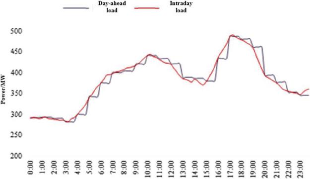
Figure 7 Load forecast curve.
The interruptible and transferable high-load energy consumption units participate in the day-ahead 24-hour optimization scheduling, while the power-variable high-load energy consumption units engage in the intra-day 15-minute optimization scheduling. The initial operating power of high-load energy-consuming equipment is its rated operating power before engaging in regulatory involvement.
6.2 Results Analysis
The day-ahead optimization scheduling method aims to minimize the overall system cost. This work employs an upgraded particle swarm optimization approach to address the two-stage optimal scheduling model for day-ahead and intra-day planning. Figure 8 depicts the wind power production curve following the integration of interruptible and transferable high-load energy consumption units in the system’s day-ahead control.
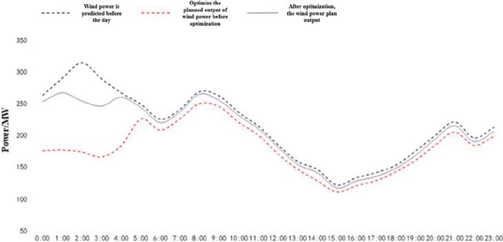
Figure 8 Wind power optimization dispatch results for the previous day.
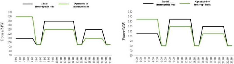
Figure 9 Interruptible and transferable operation of high energy loads.
The day-ahead wind power forecast curve in Figure 8 illustrates considerable fluctuations in wind power generation, varying between 120 and 320 MW. The optimal wind power generation is between 00:00 and 06:00, whilst the minimal output period is from 14:00 to 20:00. Therefore, the peak and trough timings of the load power forecast curve shown in Figure 6 are exactly the opposite of what they should be. This signifies that wind power production exhibits considerable unpredictability and a counter-peaking trait, which substantially exacerbates the peak control demands on conventional units within the system, significantly impeding large-scale wind power integration.
Figure 9 illustrates the electricity usage subsequent to the involvement of interruptible and transferable high-load energy consumption units in the optimization scheduling. Figure 8 illustrates that between 00:00 and 06:00, when wind power absorption is impeded, The day-ahead wind power production plan is improved by interruptible and transferable high-load energy consumption units augmenting their electricity demand to counteract the counter-peaking impacts of wind power.
In the standard scheduling mode, the total wind curtailment throughout the day-ahead scheduling period amounts to 824.48 MWh. After incorporating interruptible and transferable high-load energy consumption units into the day-ahead optimization plan, total wind curtailment for the same period decreased to 229.08 MWh, yielding an 11.56% reduction in the curtailment rate. The day-ahead wind curtailment predominantly occurs during the late-night hours from 00:00 to 04:00, when wind power is plentiful. As electricity consumption rises throughout the day and wind power variability diminishes, the phenomena of wind curtailment basically ceases to exist. This illustrates that including high-load energy consumption units into the optimization scheduling strategy can substantially alleviate the impeded absorption of wind power.
The intra-day scheduling is further improved based on the outcomes of the day-ahead optimization scheduling. Compared to the day-ahead prediction, the intra-day 15-minute wind power output projection is more accurate. Power-variable high-load energy consumption units can respond quickly to variations in wind power when they are used in intra-day optimization scheduling because of their capacity to make continuous changes at short intervals. This lessens the impact of wind curtailment brought on by variations in the intra-day and day-ahead wind power projections.
The output of power-variable high-load energy consumption units and the outcomes of intra-day wind power optimization are displayed in Figure 10.
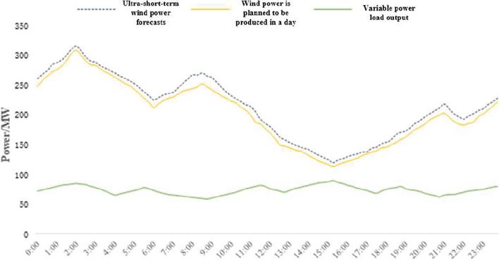
Figure 10 Intraday wind power optimization and continuous type high load energy output.
The power-variable high-load energy consumption units may actively adapt to variations in wind power production by adjusting their output during the peak wind period, which is from 00:00 to 04:00, as shown in Figure 10, which contrasts with the day-ahead wind power output plan curve. This optimizes the absorption of reduced wind power and increases the system’s capacity for wind power consumption by addressing the inadequate adjustment capabilities of thermal power plants and interruptible, transferable high-load energy consumption units. The curtailed distributed wind power in the distribution network drops from 229.08 MW (as predicted in the day-ahead schedule) to 138.97 MW (a curtailment rate of 2.7%, below the national average) when the continuously adjustable high-load energy consumption units are incorporated into the intra-day optimization scheduling. This guarantees the best possible use of wind energy resources and drastically reduces wind power curtailment.
Figures 11 and 12 show the thermal power plant’s output results from both the conventional scheduling scheme and the suggested day-ahead and intra-day two-stage optimization scheduling technique.
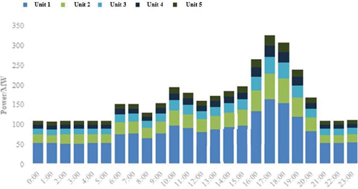
Figure 11 Thermal power unit output before optimization.
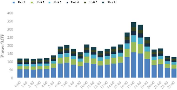
Figure 12 Optimized thermal unit output.
Figure 10 illustrates that when high-load energy consumption units abstain from system management, thermal power plants sustain their minimum production for 9 periods, resulting in significant wind power curtailment. Following the integration of high-load energy consumption units into the system regulation alongside traditional thermal power plants, as illustrated in Figure 11, the duration of times in which thermal power plants sustain their minimum output is diminished to 5. Moreover, the energy consumption of high-load units can be reduced to restrict the output of thermal power plants during periods of less wind power generation and increased load demand (16:00 to 20:00). This lowers the peak-valley load differential, improves system safety and stability, and lowers the carbon emissions and operating costs of thermal power plants.
Table 4 displays the system running expenses prior to and following optimization.
Table 4 Information on system running expenses
| Thermal | High | Wind | Total | |
| Project | Power Units | Energy Loads | Curtailment | Cost |
| Before optimization | 125.34 | 0 | 30.48 | 155.82 |
| After optimization | 117.49 | 18.66 | 8.47 | 144.62 |
Table 4 demonstrates that, subsequent to the execution of the proposed two-stage day-ahead and intra-day optimization scheduling strategy, the regulation expenses for high-load energy consumption units in the distribution network increase, whereas the operational costs of thermal power plants and wind curtailment expenses significantly decrease. As a result, the total system expense decreases by 112,000 yuan. Furthermore, the wind power curtailment administered by high-load energy consumption units increases the capacity of these units, hence enhancing the income from high-load energy products.
The proposed two-stage day-ahead and intra-day distribution network optimization scheduling strategy, which involves high-load energy consumption units, effectively lowers thermal power plant operating costs, diminishes carbon emissions, mitigates peak-regulation demands during wind power fluctuations, and enhances revenue for high-load energy consumption units, all while incurring only a slight rise in regulation costs for high-load energy consumption. This method improves the incorporation of distributed renewable energy in the distribution network.
In order to analyze the internal mechanism of the system cost change more deeply, the contribution rate of the cost change of each part to the total cost change is further calculated. The change in the total cost is 112,000 yuan, which is obtained by subtracting the total cost after optimization from the total cost before optimization. Among them, the change in thermal power cost is 78,500 yuan, and its contribution rate to the total cost change is approximately 70.09%; the change in the regulation cost of high-energy-consuming loads is 186,600 yuan, with a contribution rate of approximately 166.61%; the change in wind curtailment cost is 220,100 yuan, with a contribution rate of approximately 196.52%. It can be seen that the decrease in thermal power cost and wind curtailment cost is the main driving factor for the reduction of the total cost. Although the regulation cost of high-energy-consuming loads has increased, the increase range is relatively small, which significantly reduces the total system cost as a whole. This verifies the effectiveness of the optimized scheduling strategy proposed in this paper in terms of cost control.
7 Conclusion
This study investigated the integration of distributed renewable energy (DRE) into the distribution network under the background of the dual uncertainties of “source-load” caused by the large-scale integration of DRE. It focused on solving the problem that the insufficient peak regulation capacity of the distribution network affects the consumption of DRE. The regulatory characteristics of different high-energy-consuming load units were explored in depth, and a two-stage day-ahead and intra-day optimization scheduling strategy using high-energy-consuming load units was proposed to absorb curtailed wind power. The effectiveness of this method was verified through simulation analysis. The specific research results are as follows:
(1) Multi-type Load Collaborative Scheduling: In this study, interruptible, transferable, and variable-power high-energy-consuming load units were incorporated into the day-ahead and intra-day optimization scheduling based on their operating characteristics and those of wind power, giving full play to the multi-time-scale characteristics of high-energy-consuming load units. Some previous studies only considered the participation of a single type of high-energy-consuming load in scheduling. In contrast, this study integrates multiple types of loads, which can more comprehensively address the uncertainty of wind power. For example, during periods of low load and high wind power generation, interruptible and transferable loads can be coordinated and adjusted to better absorb wind power, while a scheduling strategy based on a single load type may not be able to respond to complex situations as flexibly.
(2) Optimization of the Scheduling Model: A two-stage day-ahead and intra-day optimization scheduling model that includes high-energy-consuming load units was established to minimize the total system cost. A collaborative scheduling strategy for curtailed wind power and high-energy-consuming loads was developed, and the effectiveness of the model was evaluated using an improved particle swarm optimization algorithm. Some previous studies did not distinguish between different time scales for scheduling optimization. In this study, through two-stage optimization scheduling, the start/stop of units and the scheduling quantity of some loads are determined in the day-ahead stage, and the variable-power loads are dynamically adjusted according to ultra-short-term wind power forecasts in the intra-day stage, enabling more precise optimization of the system cost. When dealing with wind power fluctuations and load changes, the cost control effect of this study is better.
(3) Enhancing the Consumption Capacity of Renewable Energy: Implementing the optimization scheduling strategy recommended in this study can effectively alleviate the consumption problem of renewable energy when it is integrated into the distribution network. Incorporating high-energy-consuming load units into the distribution network scheduling can ensure the consumption of DRE while reducing the system operating cost. Some previous studies used energy storage devices and other methods to consume wind power, which required substantial additional investment. In contrast, this study uses high-energy-consuming loads to consume wind power without such investment, which has an advantage in economic cost. Moreover, high-energy-consuming loads are widely distributed and have a fast adjustment response speed, which can more timely respond to wind power fluctuations and improve the efficiency of wind power consumption. In summary, compared with previous similar studies, this study has significant advantages in multi-type load collaborative scheduling, refinement of the scheduling model, and economic cost control, providing a more effective solution for the efficient consumption of DRE in the distribution network.
Acknowledgement
This study is funded by the project of Power Grid Planning Research Center of Guizhou Power Grid Co., Ltd.-Research and Application of Digital Integration Planning Technology for County Distribution Network Resources-Project 5: Research and Development and Application of Digital Integration Planning Assistant Decision System for County Distribution Network Resources (GZKJXM20222472).
References
[1] Z. Liu, S. Wang, M. Q. Lim, M. Kraft, and X. Wang. (2021). Game theory-based renewable multi-energy system design and subsidy strategy optimization. Adv. Appl. Energy, 2, page 100024.
[2] M. Zhang, Z. Yang, L. Liu, and D. Zhou. (2021). Impact of renewable energy investment on carbon emissions in China - An empirical study using a nonparametric additive regression model. Sci. Total Environ., 785, page 147109.
[3] X. Wang, Z. Y. Zhang, S. H. Zhang, and S. Q. Zhang. (2024). Game Analysis of Electricity Market With Considerations of Leasing-based Energy StorageSharing for Renewable Generators. Power Syst. Technol., 48, pages 3269–3277.
[4] X. Wang, K. Zhang, and S. H. Zhang. (2018). Joint Equilibrium Analysis of Day-ahead Electricity Market and DRX Market Considering Wind Power Bidding. Proc. CSEE, 38, pages 5738–5750+5930.
[5] L. Sigrist, E. Lobato, and L. Rouco. (2013). Energy storage systems providing primary reserve and peak shaving in small isolated power systems: An economic assessment. Int. J. Electr. Power Energy Syst., 53, pages 675–683.
[6] H. Zhou, L. Lu, M. Wei, L. Shen, and Y. Liu. (2024). Robust Scheduling of a Hybrid Hydro/Photovoltaic/Pumped-Storage System for Multiple Grids Peak-Shaving and Congestion Management. IEEE Access, 12, pages 22230–22242.
[7] J. Li, X. Li, F. Wei, P. Yan, J. Liu, and D. Yu. (2023). Research on Techno-economic Evaluation of New Type Compressed Air Energy StorageCoupled With Thermal Power Unit. Proc. CSEE, 43, pages 9171–9183.
[8] G. Cheng et al. (2021). Synergistic Performance and Combination Design of Coupling ofRenewable Energy and Thermal Power. Power Syst. Technol., 45, pages 2178–2191.
[9] A. Mnatsakanyan, H. Albeshr, A. A. Marzooqi, and E. Bilbao. (Year). Blockchain-Integrated Virtual Power Plant Demonstration. 2020 2nd International Conference on Smart Power & Internet Energy Systems (SPIES).
[10] Z. Yi, Y. Xu, H. Wang, and L. Sang. (2021). Coordinated Operation Strategy for a Virtual Power Plant With Multiple DER Aggregators. IEEE Trans. Sustain. Energy, 12, pages 2445–2458.
[11] X. Bai, Y. Fan, T. Wang, Y. Liu, X. Nie, and C. Yan. (2022). Non-intrusive load fluctuation detection based on voting variance. Electr. Power Autom. Equip., 42, pages 102–110.
[12] X. Guo, C. Cai, H. Shi, Y. Xie, and Y. Zhang. (Year). Robust based optimal operation model of virtual power plant in electricity market. 2021 China International Conference on Electricity Distribution (CICED).
[13] Y. Wang, G. Cai, D. Yang, and L. Wang. (2021). Optimization of Wind - thermal Bundled Capacity Ratio with SmallSignal Stability Constraints. Proc. CSU-EPSA, 33, pages 131–137.
[14] J. Li, F. Li, P. Wang, H. Li, and M. Chen. (2021). Analysis of Improving Transient Stability of DFIG - type Wind - thermal Binding System byCurrent - limiting SSSC. Proc. CSU-EPSA, 33, pages 68–76.
[15] Z. Wang, L. Liu, Z. Liu, S. Wang, and Z. Yu. (2014). Optimal Configuration of Wind & Coal Power Capacity and DC PlacementBased on Quantum PSO Algorithm. Proc. CSEE, 34, pages 2055–2062.
[16] L. Li et al. (2017). Impact of wind farms for wind-thermal-bundled powertransmitted system on transient out-of-step of power grid. Renew. Energy, 35, pages 884–892.
[17] J. An, S. Zhang, G. Mu, C. Zheng, and Y. Zhou. (2017). Study of dfig wind farm real power dispatching mode influence on transient stability of wind-thermalbundled power system. Acta Energ. Sol. Sin., 38, pages 1391–1396.
[18] X. Xu, H. Jia, D. Wang, D. C. Yu, and H.-D. Chiang. (2015). Hierarchical energy management system for multi-source multi-product microgrids. Renew. Energy, 78, pages 621–630.
[19] L. Yang et al. (2022). Optimal Scheduling Method for Coupled System Based on Ladder-type Ramp Rate ofThermal Power Units. Proc. CSEE, 42, pages 153–164.
Biographies
JinSen Liu graduated from the School of Electrical Engineering, Guizhou University with a bachelor’s degree. After graduation, he worked at the Power Grid Planning and Research Center of Guizhou Power Grid Co., Ltd. His main research domainds include distribution network planning and new power systems. His current professional title is an engineer.
Ning Luo graduated from from the School of Electrical Engineering, Guizhou University with a master’s degree. After graduation, she worked at the Power Grid Planning and Research Center of Guizhou Power Grid Co., Ltd. Her main research domains include distribution network planning and new power systems. Her current professional title is senior engineer.
Ludong Chen graduated from the School of Electrical Engineering, Guizhou University with a bachelor’s degree. After graduation, he worked at the Power Grid Planning and Research Center of Guizhou Power Grid Co., Ltd. His main research domains include distribution network planning and newpower systems. His current professional title is engineer.
Fei Zheng graduated from the School of Electrical Engineering, Guizhou University with a Master’s degree. After graduation, he worked at the Power Grid Planning and Research Center of Guizhou Power Grid Co., Ltd. His main research domains include distribution network planning and new power systems. His current professional title is assistant engineer.
Chang Xu graduated from the School of Urban Science and Technology, Chongqing University with a bachelor’s degree. After graduation, she worked at the Guizhou Power Grid Co., Ltd. Her main research domains include Distribution network planning and digitalization of power grid. Her current professional title is economist.
Distributed Generation & Alternative Energy Journal, Vol. 40_1, 109–140.
doi: 10.13052/dgaej2156-3306.4015
© 2025 River Publishers