Strategy Improved Pelican Algorithm Optimization ELM for Short-Term Electricity Load Forecasting

Guozhen Ma, Shiyao Hu, Ning Pang and Qiang Zhou^*

Economic and Technological Research Institute, State Grid Hebei Electric Power Co., Ltd., Shijiangzhuang, China
E-mail: 18386043022@163.com
*Corresponding Author

Received 13 January 2025; Accepted 15 February 2025

Abstract

When applying extreme learning machine (ELM) to short-term power load forecasting, its randomized weights and thresholds result in relatively low prediction accuracy and stability. Meanwhile, the pelican optimization algorithm (POA) suffers from the limitation of easily falling into local optima. To address these issues, this study proposes an improved pelican optimization algorithm (IPOA) to optimize ELM for short-term power load forecasting. The proposed method first incorporates an improved one-dimensional chaotic mapping (1-SCEC), Levy flight strategy, and adaptive weight strategy to enhance the optimization capability of POA, with the superiority of IPOA validated through two standard test functions. Subsequently, IPOA is employed to optimize ELM parameters, establishing an IPOA-ELM-based short-term power load forecasting model. The feasibility of the IPOA-ELM model is verified using actual power load forecasting data from an Australian region. Experimental results demonstrate that the proposed model achieves closer prediction results to actual loads for both weekends and weekdays, exhibiting superior prediction accuracy and stability compared to alternative methods.

Keywords: Short-term electricity load forecasting, pelican optimization algorithm, extreme learning machine, forecasting accuracy, stability, load forecasting model.

1 Introduction

Under the impetus of the “dual carbon” goals, the evolving modern power system has witnessed an increasing integration of distributed energy resources into the power grid. This integration has intensified the volatility and complexity of load sequences, further complicating power load forecasting and potentially impacting the secure and stable operation of power systems. Reliable and continuous power supply is crucial for economic development and residential life, making the establishment of accurate and stable power load forecasting models essential for improving grid dispatch efficiency.

Power load forecasting can be categorized based on time horizons into short-term, medium-term, and long-term predictions. Short-term load forecasting, focusing on predictions ranging from several hours to several days, plays a vital role in real-time grid management and power system stability enhancement. Current short-term load forecasting methodologies encompass statistical approaches and machine learning techniques. Statistical methods include time series analysis, Kalman filtering, and multivariate linear regression. While these traditional forecasting methods offer simplicity and computational efficiency, they exhibit limitations in prediction accuracy and complex data feature extraction, falling short of modern power system requirements.

With the rapid advancement of artificial intelligence and computational capabilities, researchers have increasingly adopted machine learning approaches for power load forecasting, primarily employing long short-term memory (LSTM) networks, support vector machines (SVM), and extreme learning machines (ELM). Previous studies have proposed various improvements: an enhanced chimpanzee algorithm-optimized LSTM model improved prediction accuracy but suffered from parameter redundancy and overfitting issues; an improved SVM model demonstrated optimal accuracy and stability but faced challenges in kernel parameter selection and lengthy training times. While ELM offers easy implementation and rapid learning capabilities, its randomly generated weights and thresholds result in reduced prediction accuracy and stability, making the optimization of ELM through appropriate intelligent algorithms a current research focus in short-term power load forecasting.

Based on these analyses, this study proposes a short-term power load forecasting method using an improved pelican optimization algorithm (IPOA) to optimize ELM. The methodology first enhances the traditional pelican optimization algorithm (POA) by incorporating improved one-dimensional chaotic mapping (1-SCEC) for population initialization, integrating Levy flight strategy for position updates, and introducing adaptive weight factors in the exploration phase to enhance escape from local optima. The IPOA algorithm’s performance is validated through test functions before being applied to optimize ELM’s weights and thresholds, establishing an IPOA-ELM short-term power load forecasting model. Finally, comparative experiments with other models demonstrate the effectiveness and feasibility of the proposed model in short-term power load forecasting.

2 Improved Pelican Algorithm and Its Performance Verification

2.1 Pelican Optimization Algorithm

The Pelican Optimization Algorithm, introduced by Pavel Trojovskı et al. in early 2022, is a novel intelligent algorithm inspired by pelicans’ foraging behavior. In the POA algorithm, each pelican’s position information corresponds to a potential solution. The mathematical expression for initializing the pelican population’s position is shown in the following equation:

$$X_{i,j}=l_j+\mathit{rand}(u_j-l_j),i=1,2,\mathrm{\dots },n,j=1,2,\mathrm{\dots },m$$

(1)

where $X_{i,j}$ represents the position of the i-th pelican in the j-th dimension, n denotes the number of pelicans, m is the number of variables, and $u_j$ and $l_j$ represent the upper and lower bounds of the j-th dimension problem, respectively.

At this stage, the pelican population X and the objective function matrix can be represented by the following equations, respectively:

$$X={\left[\begin{array}{c}\hfill X_1\hfill \\ \hfill \mathrm{⋮}\hfill \\ \hfill X_i\hfill \\ \hfill \mathrm{⋮}\hfill \\ \hfill X_n\hfill \end{array}\right]}_{n\times m}={\left[\begin{array}{ccccc}\hfill X_{1,1}\hfill & \hfill \mathrm{\cdots }\hfill & \hfill X_{1,j}\hfill & \hfill \mathrm{\cdots }\hfill & \hfill X_{1,m}\hfill \\ \hfill \mathrm{⋮}\hfill & \hfill \mathrm{\ddots }\hfill & \hfill \mathrm{⋮}\hfill & & \hfill \mathrm{⋮}\hfill \\ \hfill X_{i,1}\hfill & \hfill \mathrm{\cdots }\hfill & \hfill X_{i,j}\hfill & \hfill \mathrm{\cdots }\hfill & \hfill X_{i,m}\hfill \\ \hfill \mathrm{⋮}\hfill & & \hfill \mathrm{⋮}\hfill & \hfill \mathrm{\ddots }\hfill & \hfill \mathrm{⋮}\hfill \\ \hfill X_{n,1}\hfill & \hfill \mathrm{\cdots }\hfill & \hfill X_{n,j}\hfill & \hfill \mathrm{\cdots }\hfill & \hfill X_{n,m}\hfill \end{array}\right]}_{n\times m}$$

(2)

$$F=\left[\begin{array}{c}\hfill F_1\hfill \\ \hfill \mathrm{⋮}\hfill \\ \hfill F_i\hfill \\ \hfill \mathrm{⋮}\hfill \\ \hfill F_n\hfill \end{array}\right]=\left[\begin{array}{c}\hfill F(x_1)\hfill \\ \hfill \mathrm{⋮}\hfill \\ \hfill F(x_i)\hfill \\ \hfill \mathrm{⋮}\hfill \\ \hfill F(x_n)\hfill \end{array}\right]$$

(3)

where $X_i$ and $F_i$ represent the position and corresponding objective function value of the i-th pelican, respectively.

The foraging behavior of the pelican population is divided into exploration and exploitation phases:

(1) Exploration Phase During this phase, pelicans first search for prey. When prey appears within their visual range, pelicans identify the foraging area and rapidly approach the prey. The position update of pelicans during this process can be expressed by the following equation:

$$X_{i,j}^{P_1}=\{\begin{array}{cc}{X}_{i,j}+rand(P_j-I\cdot X_{i,j}),\hfill & F_P{F}_i\hfill \\ X_{i,j}+rand(X_{i,j}-P_j),\hfill & \mathrm{else}\hfill \end{array}$$

(4)

where $X_{\mathrm{i},\mathrm{j}}^{P_1}$ denotes the position of the i-th pelican in the j-th dimension during the first phase, P${}_j$ represents the position of prey in the j-th dimension, I is a random number of either 1 or 2, $F_p$ represents the objective function value of the prey, and rand is a random number between 0 and 1.

If the objective function value improves, the pelican accepts the new position; otherwise, it rejects the update. This process, known as effective pelican updating, is expressed by the following equation:

$$X_i=\{\begin{array}{cc}{X}_i^{P_1},\hfill & F_i^{P_1}{F}_i\hfill \\ X_i,\hfill & \mathrm{else}\hfill \end{array}$$

(5)

where $X_{\mathrm{i}}^{P_1}$ represents the position of the i-th pelican during the first phase, and $F_{\mathrm{i}}^{P_1}$ denotes the objective function value in the first phase.

(2) Exploitation Phase When pelicans reach the water surface, they use their wings to strike the water, enabling them to collect prey in their throat pouch. This hunting method increases the success rate in the foraging area, enhancing the local search capability of the POA algorithm. The exploitation phase can be expressed by the following equation:

$$X_{i,j}^{P_2}=X_{i,j}+R\cdot (1-t/T)\cdot (2\mathit{rand}-1)\cdot X_{i,j}$$

(6)

where $X_{\mathrm{i},\mathrm{j}}^{P_2}$ represents the position of the i-th pelican in the j-th dimension during the second phase, t is the current iteration number, T is the maximum number of iterations, and $R=0.2$.

As in the exploration phase, effective updating is used to accept or reject new positions, as expressed by the following equation:

$$X_i=\{\begin{array}{cc}{X}_i^{P_2},\hfill & F_i^{P_2}{F}_i\hfill \\ X_i,\hfill & \mathrm{else}\hfill \end{array}$$

(7)

where $X_{\mathrm{i}}^{P_2}$ represents the position of the i-th pelican in the second phase, and $F_{\mathrm{i}}^{P_2}$ denotes the objective function value in the second phase.

2.2 Improved Pelican Optimization Algorithm

While the traditional pelican algorithm offers advantages such as simple structure and high accuracy, it shares a common limitation with other swarm intelligence optimization algorithms: potentially missing optimal solutions during initialization. Additionally, the POA algorithm tends to fall into local optima during the exploration phase. Therefore, this paper proposes improvements through 1-SCEC, Levy flight strategy, and adaptive weight strategy.

(1) Improved One-dimensional Chaotic Mapping Chaotic mapping With its excellent random characteristics, can influence the entire iteration process when used for population initialization. This is particularly effective in finding global optimal solutions when multiple local solutions exist within the algorithm’s search space. Chebyshev chaotic mapping and Sine chaotic mapping are common one-dimensional chaotic mappings, with their spatial distributions shown in Figures 1 and 2, respectively.

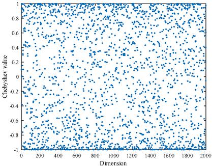
Figure 1 Spatial distribution of Chebyshev mapping.

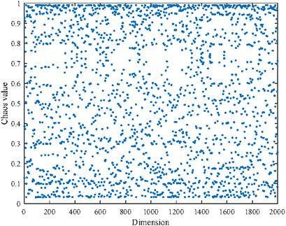
Figure 2 Spatial distribution of sine mapping

The mapping equations for Chebyshev chaotic mapping and Sine chaotic mapping are shown in the following equations:

$$x_{n+1}=\cos (k\arccos x_n),x_n\in [-1,1]$$	(8)
$$x_{n+1}=a\sin (\pi x_n)/4,x_n\in [0,1]$$	(9)

where k represents the order, typically set to 4, with the model entering a chaotic state when k exceeds 2. a is the control parameter, and $x_{n+1}$ is the output value.

While one-dimensional chaotic mapping offers simplicity and computational efficiency, it faces challenges such as uneven sequence point distribution and limited mapping parameter ranges. Therefore, this paper combines these two chaotic mappings through composite transformation to obtain an improved one-dimensional chaotic mapping, expressed by the following equation:

$x_{n+1}$	$=\cos [\pi {(1-2(\cos (\lambda \arccos (x_n))))}^2\cdot (2\exp (x_n)$
	$\mathrm{\hspace{1em}}+\exp (-x_n))+\pi (4-\lambda )/4\cdot \sin (\pi x_n)(2\exp (x_n)$
	$\mathrm{\hspace{1em}}+\exp (-x_n))],x{}_n\in [0,1]$	(10)

where $\lambda$ is the chaotic parameter valued between 0 and 4, set to 4 in this study. The mapping spatial distribution of 1-SCEC is shown in Figure 3.

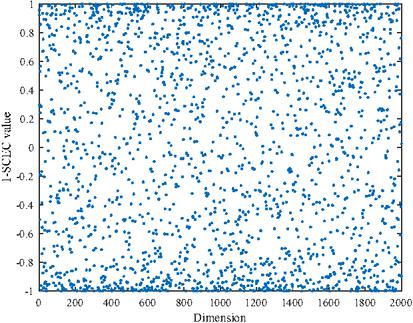
Figure 3 Spatial distribution of 1-SCEC mapping.

(2) Levy Flight Strategy The Levy flight strategy, which mimics natural flight patterns, is incorporated into the pelican algorithm to enhance the population’s natural adaptability and global search capability. Therefore, this study integrates the Levy flight strategy into the pelican position update process to improve global search capabilities and the ability to escape local optima. The calculation equations for the Levy flight strategy are shown in the following equations:

$$\mathrm{Levy}=\frac{\mu }{{|v|}^{\frac{1}{\beta }}}$$	(11)
$$\sigma ={\left(\frac{\mathrm{\Gamma }(1+\beta )\times \sin (\pi \beta /2)}{\mathrm{\Gamma }((1+\beta /2)\times \beta \times 2^{(\beta -1)/2})}\right)}^{\frac{1}{\beta }}$$	(12)

where $\beta =1.5$, and $\mu$ and v are parameters following normal distribution.

(3) Adaptive Weight Strategy The adaptive weight strategy optimizes model performance through dynamic weight adjustment while balancing global and local search capabilities. To address the tendency of pelicans falling into local optima during the exploration phase, an adaptive weight factor $\omega$ is introduced in the position update during this phase, as expressed by the following equation:

$$\omega =e^{-\frac{10t}{{\mathrm{T}}_{\max }}}$$

(13)

The new pelican position update shown in the following equation:

$$X_{i,j}^{P_1}=\{\begin{array}{cc}\omega \cdot X_{i,j}+rand(P_j-I\cdot X_{i,j}),\hfill & F_P{F}_i\hfill \\ \omega \cdot X_{i,j}+rand(X_{i,j}-P_j),\hfill & \mathrm{else}\hfill \end{array}$$

(14)

2.3 Performance Verification of Improved Pelican Optimization Algorithm

To validate the optimization effectiveness of the IPOA algorithm, experiments were conducted using Sphere and Schwefel functions, comparing against POA, dung beetle optimizer (DBO), aquila optimizer (AO), and northern goshawk optimization (NGO) algorithms. All algorithms were configured with 500 iterations and 30 dimensions. The Sphere function, visualized in Figure 4, exhibits a smooth concave surface with only a global optimum and no local optima, making it suitable for testing convergence speed. The Sphere function is expressed by the following equation:

$$f_1(x)=\sum _{i=1}^{30}{x}_i^2$$

(15)

where $x\in [-100,100]$, with an optimal solution of 0.

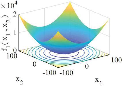
Figure 4 Sphere test function surface.

The Schwefel function, a typical deceptive problem used to test algorithms’ ability to escape local optima and find global optimal solutions, is visualized in Figure 5 and mathematically expressed by the following equation:

$$f_2(x)=\sum _{i=1}^{30}|x_i|+\prod _{i=1}^{30}|x_i|$$

(16)

where $x\in [-10,10]$, with an optimal solution of 0.

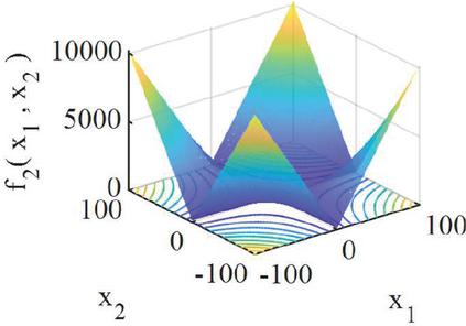
Figure 5 Schwefel test function surface.

To ensure experimental validity, ten trials were conducted for each of the five algorithms on both test functions using MATLAB. The most representative results are shown in Figures 6 and 7. Algorithm performance was evaluated using best solution (best), mean value (mean), and standard deviation (std), with comparative results presented in Table 1.

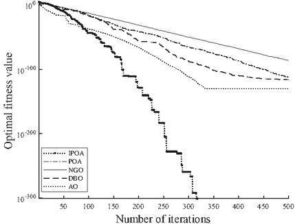
Figure 6 Sphere test results comparison.

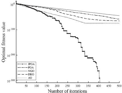
Figure 7 Schwefel test results comparison.

Table 1 Optimization results comparison

Function	Evaluation	IPOA	POA	DBO	AO	NGO
Type	Metrics	Algorithm	Algorithm	Algorithm	Algorithm	Algorithm
	best	0	$2.38\times {10}^{-113}$	$5.51\times {10}^{-155}$	$1.73\times {10}^{-162}$	$7.47\times {10}^{-90}$
Sphere	mean	0	$3.15\times {10}^{-106}$	$3.44\times {10}^{-119}$	$6.59\times {10}^{-138}$	$4.72\times {10}^{-88}$
	std	0	$6.63\times {10}^{-106}$	$9.81\times {10}^{-119}$	$2.08\times {10}^{-137}$	$5.48\times {10}^{-88}$
	best	0	$4.59\times {10}^{-57}$	$6.41\times {10}^{-80}$	$3.06\times {10}^{-79}$	$8.29\times {10}^{-47}$
Schwefel	mean	0	$2.52\times {10}^{-52}$	$2.91\times {10}^{-66}$	$5.44\times {10}^{-56}$	$2.07\times {10}^{-45}$
	std	0	$7.31\times {10}^{-52}$	$6.14\times {10}^{-66}$	$1.72\times {10}^{-55}$	$3.93\times {10}^{-45}$

The proximity of the optimal solution to 0 indicates higher algorithmic precision, with mean values describing overall algorithmic performance lower values indicating better performance. Standard deviation characterizes algorithmic stability, with smaller values demonstrating higher stability. As shown in Figures 6, 7, and Table 1, the IPOA algorithm achieves smaller optimal solutions compared to other algorithms, finding the optimal solution of 0 for both Sphere and Schwefel functions, indicating higher solving precision. Additionally, the IPOA algorithm demonstrates lower mean values and standard deviations compared to other algorithms, indicating superior overall performance and stability.

3 Short-term Power Load Forecasting Model

3.1 Extreme Learning Machine

The extreme learning machine (ELM) shares the same structure as a single-hidden layer feedforward neural network, comprising input, hidden, and output layers, with advantages of simple structure and rapid parameter optimization, as shown in Figure 8.

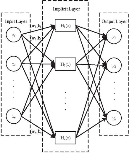
Figure 8 Structural diagram of ELM.

Given a dataset $\{x_i,t_i|x_i\in R_n,t_i\in R_n,i=1,2,\mathrm{\dots },n\}$, where $x_i$ represents input and $t_i$ represents output, and letting $g(x)$ be the activation function, the output matrix $H$ can be expressed by the following equation:

$$\mathit{H}=\left[\begin{array}{ccc}\hfill g({\omega }_1\cdot x_1+b_1)\hfill & \hfill \mathrm{\dots }\hfill & \hfill g({\omega }_l\cdot x_1+b_l)\hfill \\ \hfill \mathrm{⋮}\hfill & \hfill \mathrm{\dots }\hfill & \hfill \mathrm{⋮}\hfill \\ \hfill g({\omega }_1\cdot x_n+b_1)\hfill & \hfill \mathrm{\dots }\hfill & \hfill g({\omega }_l\cdot x_n+b_l)\hfill \end{array}\right]n\times l$$

(17)

where ${\omega }_i$ is the input weight, $b_i$ is the input threshold. n, l, and m are the number of nodes in the input layer, hidden layer, and output layer, respectively.

The weight value $\beta$ connecting hidden and output layer nodes by the following equation:

$$\mathit{\beta }=\left[\begin{array}{c}\hfill {\beta }_1^T\hfill \\ \hfill \mathrm{⋮}\hfill \\ \hfill {\beta }_i^T\hfill \\ \hfill \mathrm{⋮}\hfill \\ \hfill {\beta }_l^T\hfill \end{array}\right]l\times m$$

(18)

The output $H_i(x)$ of the i-th hidden layer by the following equation:

$$H_{\mathrm{i}}(x)=g({\omega }_i,b_i,x)=g({\omega }_{i}x+b_i)$$

(19)

The mathematical model of ELM is expressed by the following equation:

$${\mathit{T}}^{*}=\sum _{i=1}^n\mathit{\beta }g({\omega }_i,b_i,x)$$

(20)

where $T^{*}$ is the target output matrix.

Since the weights and thresholds of ELM are randomly generated, the objective function is solved by minimizing the approximate squared error, which can be expressed as the following equation:

$$\min |H\mathit{\beta }-{\mathit{T}}^{*}|$$

(21)

Finally, the optimal solution of the objective function is obtained through matrix theory, as shown in the following equation:

$${\mathit{\beta }}^{*}={\mathit{H}}^{+}{\mathit{T}}^{*}={({\mathit{H}}^{\mathrm{T}}\mathit{H})}^{-1}{\mathit{H}}^{\mathrm{T}}{\mathit{T}}^{*}$$

(22)

where $\beta$ is the optimal solution, and $H^{+}$ is the Moore-Penrose generalized inverse of matrix H.

3.2 IPOA-ELM Prediction Model

The weights and thresholds significantly influence the prediction performance of ELM, and given that the values of weight $\omega$ and threshold b are randomly generated, this leads to instability in ELM results. Therefore, this paper employs the IPOA algorithm to optimize ELM, thereby enhancing its performance in power load forecasting. The flowchart of ELM optimization using IPOA is illustrated in Figure 9.

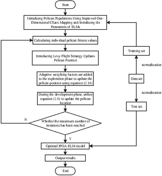
Figure 9 Flowchart of IPOA-ELM.

The specific steps of ELM optimization using IPOA algorithm are as follows:

Step 1: Collect relevant power load data and normalize the data;

Step 2: Introduce 1-SCEC in the pelican initialization phase, set the pelican population to 20, and set the maximum number of iterations to 50;

Step 3: Begin iteration by incorporating Levy flight strategy into pelican position updates. Calculate individual pelican fitness values and introduce adaptive weight factors into the pelican exploration phase, modifying the position update from Equations (4) to (14). Then pelicans enter the exploitation phase, updating positions using Equation (6). In each iteration, the current optimal position is transformed into the weights and threshold parameters of ELM, and the corresponding prediction error is calculated as the fitness value to guide the evolution direction of the population;

Step 4: Check if the model meets the termination conditions. If not, repeat the cycle; if yes, output the optimal weights and thresholds to ELM, establish the optimal IPOA-ELM power load prediction model and evaluate results.

4 Case Study

4.1 Data Preprocessing

This study selects power load data from a region in Australia from January 1, 2007 (Monday) to March 4, 2007 (Sunday) as the experimental dataset. The sampling interval is 30 minutes, resulting in 48 sampling points per day, and the data includes 5 feature factors (dry-bulb temperature, dew point temperature, wet-bulb temperature, humidity, electricity price) and power load data. To verify IPOA-ELM model’s prediction capability for weekends and weekdays, seven days of data are treated as one sample, with 57 samples in total, of which 56 are training sets and the last one serves as the test set. For the 56 training sets, the first 5 days’ load data serves as input and the last 2 days’ load data as output. The same processing applies to the final test set to test IPOA-ELM’s weekend prediction capability. For weekday prediction, 55 samples are designed, with 54 as training sets and the last one as the test set. In the 54 training sets, the first 2 days’ load data serves as input and the following 5 days’ load data as output. The same processing applies to the final test set to test IPOA-ELM’s weekday prediction capability. The sliding step is set to 1 day, i.e., using Monday to Friday data to predict Saturday to Sunday, using Tuesday to Saturday data to predict Sunday to next Monday, and so on. The load distribution for the final week is shown in Figure 10.

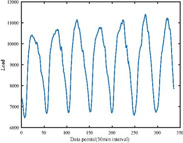
Figure 10 Load distribution profile.

To eliminate scale differences between different features, data is confined within a specific range. Before the experiment, min-max normalization is used for data preprocessing, which can be expressed by the following equation:

$$y^{\prime }=\frac{y-y_{\min }}{y_{\max }-y_{\min }}$$

(23)

where y${}^{\prime }$ is the normalized data, y is the unprocessed data, y${}_{\max }=\mathrm{\hspace{0.17em}1}$, y${}_{\min }=-1$.

4.2 Evaluation Metrics

To evaluate the performance of the proposed IPOA-ELM power load prediction model, four evaluation metrics are proposed: coefficient of determination (R2), mean absolute error (MAE), root mean square error (RMSE), and mean absolute percentage error (MAPE). These four evaluation metrics are expressed by the following equations:

$$R^2=1-\frac{{\sum }_{i=1}^n{(m_1-m_2)}^2}{{\sum }_{i=1}^n{(m_1-m^{*})}^2}$$	(24)
$$\mathit{MAE}=\frac{1}{n}\sum _{i=1}^n|(m_1-m_2)|$$	(25)
$$\mathit{RMSE}=\sqrt{\frac{1}{n}\sum _{i=1}^n{(m_1-m_2)}^2}$$	(26)
$$\mathit{MAPE}=\frac{1}{n}\sum _{i=1}^n|\frac{m_2-m_1}{m_1}|$$	(27)

where m${}_1$ is the actual value, m${}_2$ is the predicted value, m${}^{*}$ is the mean of predicted values, and n is the sample size.

4.3 Results Analysis

To demonstrate the effectiveness of the proposed IPOA-ELM power load prediction model, POA-ELM, NGO-ELM, AO-ELM, DBO-ELM, and ELM models are proposed for comparative experiments. The parameter settings for POA-ELM, NGO-ELM, AO-ELM, and DBO-ELM models are consistent with the IPOA-ELM model, while the hidden layer nodes of ELM are set to 100. The load prediction results for weekends and weekdays are shown in Figures 11 and 12, respectively. Tables 2 and 3 show the comparison of prediction accuracy results for weekends and weekdays, respectively.

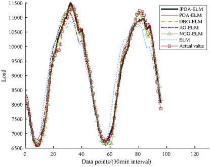
Figure 11 Weekend load prediction results.

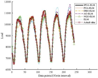
Figure 12 Weekday load prediction results.

Table 2 Comparison of prediction accuracy for weekends

Model	MAPE/%	MAE	RMSE	R2
IPOA-ELM	1.23	114.47	154.93	0.9903
POA-ELM	1.46	134.84	175.77	0.9875
DBO-ELM	1.59	152.37	194.79	0.9847
AO-ELM	2.75	251.67	295.46	0.9648
NGO-ELM	1.73	155.00	206.11	0.9829
ELM	4.47	408.16	481.60	0.9065

Table 3 Comparison of prediction accuracy for weekdays

Model	MAPE/%	MAE	RMSE	R2
IPOA-ELM	1.02	96.28	136.11	0.9902
POA-ELM	1.24	116.24	148.21	0.9883
DBO-ELM	1.64	156.40	218.94	0.9745
AO-ELM	1.94	188.98	254.11	0.9658
NGO-ELM	1.63	152.78	198.16	0.9791
ELM	4.02	397.83	474.21	0.8809

As shown in Figure 11 and Table 2, for weekends, the proposed IPOA-ELM model demonstrates better prediction performance. The coefficient of determination R2 increased by 0.28%, 0.56%, 0.74%, 2.55%, and 8.38% compared to POA-ELM, DBO-ELM, NGO-ELM, AO-ELM, and ELM, respectively. The mean absolute percentage error (MAPE) decreased by 0.23%, 0.36%, 0.5%, 1.52%, and 3.24%. The mean absolute error (MAE) decreased by 20.37, 37.9, 40.53, 137.2, and 293.69. The root mean square error (RMSE) decreased by 20.84, 39.86, 51.18, 140.53, and 326.67.

As shown in Figure 12 and Table 3, for weekdays, the proposed IPOA-ELM model continues to show better prediction performance. The coefficient of determination R2 increased by 0.19%, 1.11%, 1.57%, 2.44%, and 10.93% compared to POA-ELM, NGO-ELM, DBO-ELM, AO-ELM, and ELM, respectively. The MAPE decreased by 0.22%, 0.61%, 0.62%, 0.92%, and 3.0%. The MAE decreased by 19.96, 56.5, 60.12, 92.7, and 301.55. The RMSE decreased by 12.1, 62.05, 82.83, 118.0, and 338.1.

Furthermore, to verify the stability of the proposed model, IPOA-ELM, POA-ELM, DBO-ELM, NGO-ELM, AO-ELM, and ELM models were each run independently 10 times, and the variation curves of MAE and RMSE were used to demonstrate stability. Figures 13 and 14 show the variation curves of MAE and RMSE for each model in 10 weekend experiments, and Table 4 shows the stability analysis results for each model during weekends.

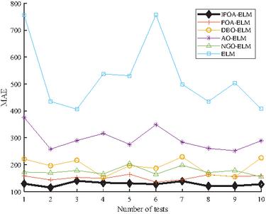
Figure 13 MAE variation curves for weekend experiments.

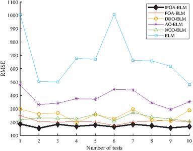
Figure 14 RMSE variation curves for weekend experiments.

Table 4 Stability analysis results for weekends

	Best	Mean	Std	Best	Mean	Std
Model	(MAE)	(MAE)	(MAE)	(RMSE)	(RMSE)	(RMSE)
IPOA-ELM	114.47	127.99	7.84	154.93	171.81	11.02
POA-ELM	134.84	152.32	9.44	175.77	206.01	17.75
DBO-ELM	152.37	193.95	29.37	194.79	251.84	37.78
AO-ELM	251.67	294.83	40.61	295.46	378.02	58.61
NGO-ELM	155.00	175.42	14.93	206.11	231.31	21.17
ELM	408.16	527.01	130.34	481.60	679.00	188.55

As shown in Figures 13, 14, and Table 4, the MAE and RMSE curves of the proposed IPOA-ELM power load prediction model are more stable. Figures 15 and 16 show the variation curves of MAE and RMSE for each model in 10 weekday experiments, and Table 5 shows the stability analysis results for each model during weekdays.

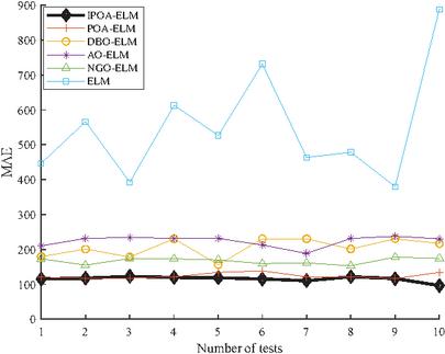
Figure 15 MAE variation curves for weekday experiments.

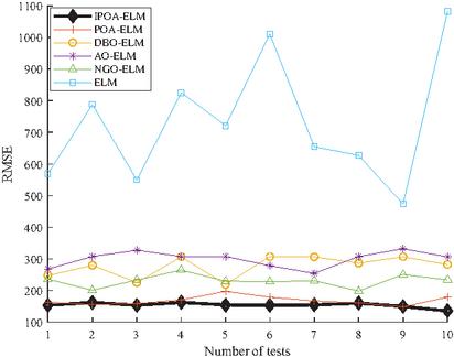
Figure 16 RMSE variation curves for weekday experiments.

Table 5 Stability analysis results for weekdays

	Best	Mean	Std	Best	Mean	Std
Model	(MAE)	(MAE)	(MAE)	(RMSE)	(RMSE)	(RMSE)
IPOA-ELM	96.28	115.28	7.58	136.11	153.91	7.55
POA-ELM	116.24	124.14	7.96	148.21	168.06	13.92
DBO-ELM	156.40	205.42	26.93	218.94	276.78	34.35
AO-ELM	188.98	223.95	15.23	254.11	299.70	24.87
NGO-ELM	152.78	166.93	9.17	198.16	230.59	19.95
ELM	397.83	548.45	159.55	474.21	730.52	198.98

As shown in Figures 15, 16, and Table 5, the MAE and RMSE curves of the IPOA-ELM model are also more stable for weekdays.

In summary, due to random weights and thresholds in ELM, its evaluation metrics show strong fluctuations and poor stability. Intelligent algorithms can effectively improve ELM’s stability in short-term power load prediction, and the proposed IPOA-ELM prediction model has the smallest standard deviation, indicating better stability for both weekends and weekdays compared to other models.

5 Conclusion

To address the problems of low prediction accuracy and poor stability of ELM in power load prediction, this paper proposes a short-term power load prediction model based on multi-strategy improved pelican optimization algorithm for optimizing ELM. The main conclusions are as follows:

(1) To address the issue of traditional pelican algorithm being prone to local optima, improvements were made by incorporating 1-SCEC, Levy flight strategy, and adaptive weight strategy. Performance verification using Sphere and Schwefel functions demonstrated that the improved pelican algorithm outperforms traditional POA, DBO, AO, and NGO algorithms in terms of both convergence accuracy and stability, effectively validating the improvement strategies.

(2) To resolve the problems of low accuracy and poor stability in ELM for short-term power load forecasting, the IPOA algorithm was employed to optimize its weights and thresholds, thereby enhancing ELM’s prediction performance. The introduction of improved chaotic mapping for population initialization, combined with Levy flight for enhanced global search capability and adaptive weight strategy to balance exploration and exploitation, effectively overcame the randomness inherent in ELM parameters.

(3) A load forecasting model based on IPOA-ELM was established and validated using actual load data from a region in Australia. Simulation results demonstrated superior performance of the proposed model in both weekday and weekend predictions. Furthermore, stability analysis through multiple independent runs showed that the proposed model exhibited minimal performance fluctuation, confirming its enhanced stability and practical significance.

Although the proposed method demonstrates favorable predictive performance and stability, the training time is relatively lengthy. Therefore, the next phase of research will focus on reducing model training time while maintaining predictive performance and stability capabilities.

References

[1] Liu J, Cong L M, Xia Y Y, et al. Short-term power load prediction based on DBO-VMD and an IWOA- BILSTM neural network combination model[J]. Power System Protection and Control, 2024, 52(08): 123–133.

[2] Li N, Jiang T, Sui X, et al. A multi-component short-term power load combination forecasting method on a time-frequency scale[J]. Power System Protection and Control, 2024, 52(13): 47–58.

[3] Liang L, Zhang Z C. Short-term load forecasting of a power system based on multi-scale feature enhanced DHTCN[J]. Power System Protection and Control, 2023, 51(10): 172–179.

[4] Cui Y, Zhu H, Wang Y J, et al. Short-term power load forecasting method based on CNN-SAEDN-Res[J]. Electric Power Automation Equipment, 2024, 44(04): 164–170.

[5] Wang Y F, Cao Y H, Sun J W, Short-term power load forecasting based on multi-strategy improved golden jackal algorithm-optimized LSTM[J]. Power System Protection and Control, 2024, 52(14): 95–102.

[6] Di S G, Liu F, Sun J Y, et al. Short Term Power Load Forecasting Based on Improved ABC and IDPC-MKELM[J]. Smart Power, 2022, 50(09): 74–81.

[7] Xiao W, Fang N, Deng X. Short-term Load Forecasting Based on VMD-LSTM-IPSO-GRU[J]. Science Technology and Engineering, 2024, 24(16): 6734–6741.

[8] Jin B J, Lin Y, Luo S X, et al. A Short-Term Load Forecasting Method Based on Load Curve Clustering and Elastic Net Analysis[J]. Electric Power, 2020, 53(09): 221–228.

[9] Wan K, Liu R Y. Application of Interval Time-Series Vector Autoregressive Model in Short-Term Load Forecasting[J]. Power System Technology, 2012, 36(11): 77–81.

[10] Liu X, Teng H, Gong Y B, et al. Short-term load forecasting based on the improved Kalman filter algorithm[J]. Electrical Measurement & Instrumentation, 2019, 56(03): 42–46.

[11] Deng D Y, Li J, Zhang Z Y, et al. Short-term Electric Load Forecasting Based on EEMD-GRU-MLR[J]. Power System Technology, 2020, 44(02): 593–602.

[12] Fan X R, Li Y C. Short-term power load forecasting based on improved Autoformer model[J]. Electric Power Automation Equipment, 2024, 44(04): 171–177.

[13] Gao C, Sun Y Q, Zhao H F, et al. Research on short-term load forecasting based on ICOA-LSTM[J]. Electronic Measurement Technology, 2022, 45(13): 88–95.

[14] Zhou S M, Duan J C, Li Y J, et al. An improved SVM short term load forecasting method for power system[J]. Journal of Shenyang University of Technology, 2023, 45(06): 661–665.

[15] Zhang S Q, Duan X N, Zhang L G, et al. Tsne Dimension Reduction Visualization Analysis and Moth Flame Optimized ELM Algorithm Applied in Power Load Forecasting[J]. Proceedings of the CSEE, 2021, 41(09): 3120–3130.

[16] Long G, Huang M, Fang L Q, et al. Short-term power load forecasting based on an improved multi-verse optimizer algorithm optimized extreme learning machine[J]. Power System Protection and Control, 2022, 50(19): 99–106.

[17] Shang L Q, Li H B, Hou Y D, et al. Short-Term Power Load Forecasting Based on Feature Selection and Optimized Extreme Learning Machine [J]. Journal of Xi’an Jiaotong University, 2022, 56(04): 165–175.

[18] PAVEL T, MOHAMMAD D. Pelican Optimization Algorithm: A Novel Nature-Inspired Algorithm for Engineering Applications[J]. Sensors, 2022, 22(3): 855–855.

[19] Zhang J X, Qiu J, Zhu Y K, et al. A new energy power grid security and stability control method based on time series convolutional residual network and pelican optimization algorithm[J]. Renewable Energy Resources, 2024, 42(06): 845–852.

[20] Li Y C, Li Y F, Wang Z, et al. Improving Pelican Optimization Algorithm by Combining 3D Spiral Motion and Hybrid Reverse Learning Strategy[J]. Science Technology and Engineering, 2024, 24(11): 4607–4617.

[21] Cheng X R, Wu L F, Yang X Z. Fractional order PID parameter tuning based on improved sparrow search algorithm[J]. Control and Decision, 2024, 39(04): 1177–1184.

[22] Chatterjee S, Roy S, Das K A, et al. Secure Biometric-Based Authentication Scheme Using Chebyshev Chaotic Map for Multi-Server Environment[J]. IEEE Transactions on Dependable and Secure Computing, 2018, 15(5): 824–839.

[23] Liu G X, Li Q, Han Z Z, et al. Journal of Ordnance Equipment Engineering[J]. Journal of Ordnance Equipment Engineering, 2023, 44(08): 240–248.

[24] Chen W, Yang P L, Wu X G. Improved Ant Lion Optimizer and Its Application in Engineering Problems[J]. Chinese Journal of Sensors and Actuators, 2023, 36(04): 565–574.

[25] Teng Z J, Fu Y S. Gu L C, et al. An optimized slime mould algorithm combining dynamic weight coefficient and Levy flight[J]. Journal of Shaanxi University of Science & Technology, 2024, 42(04): 191–198.

[26] Wu X L. Hu S, Cheng W. Multi-Objective Signal Timing Optimization Based on Improved Whale Optimization Algorithm[J]. Journal of Kunming University of Science and Technology (Natural Science), 2021, 46(01): 134–141.

[27] Li Q, Zhang X Y, Ma T J, et al. Multi-step Ahead Ultra-short Term Forecasting of Wind Power Based on ECBO-VMD-WKELM[J]. Power System Technology, 2021, 45(08): 3070–3080.

[28] Zhang D H, Sun K, He J H. Short-term Load Forecasting Based on Similar Day and Multi-model Fusion[J]. Power System Technology, 2023. 47(05): 1961–1970.

[29] Li L L, Ren Q Y, Ning N, et al. Short-term power load forecasting based on ISHO-ELM model[J]. Journal of Tiangong University, 2023, 42(03): 73–80.

Biographies

Guozhen Ma, Chief Expert at State Grid Corporation of China, is a Level 5 staff member at the Energy Development Research Center of the Economic and Technological Research Institute of State Grid Hebei Electric Power Company. He holds the title of Senior Economist and has long been engaged in research on energy and electricity economics, with a primary focus on bigdata analysis and applications in the electricity sector.

Shiyao Hu, the deputy director, Senior engineer, Energy Development Research Center, Economic and Technological Research Institute of Hebei Electric Power Company, State Grid of China, has been engaged in power grid planning for a long time, mainly focusing on distribution network planning.

Ning Pang, a senior engineer in the Energy Development Research Center of Economic and Technological Research Institute of Hebei Electric Power Co., LTD., State Grid of China. He has been engaged in power grid planning and design for a long time. Her main research direction is power big data analysis and application.

Qiang Zhou, a researcher working on new energy and power systems. His primary research focus is on the optimization analysis and application of power systems.

Distributed Generation & Alternative Energy Journal, Vol. 40_1, 85–108.
doi: 10.13052/dgaej2156-3306.4014
© 2025 River Publishers

Abstract

1 Introduction

2 Improved Pelican Algorithm and Its Performance Verification

2.1 Pelican Optimization Algorithm

2.2 Improved Pelican Optimization Algorithm

2.3 Performance Verification of Improved Pelican Optimization Algorithm

3 Short-term Power Load Forecasting Model

3.1 Extreme Learning Machine

3.2 IPOA-ELM Prediction Model

4 Case Study

4.1 Data Preprocessing

4.2 Evaluation Metrics

4.3 Results Analysis

5 Conclusion

References

Biographies