Distributed Optimization Model for Economic Dispatch of Smart Grid

Jinlin Chen^* and Nianwei Hu

School of Automation Engineering, Henan Polytechnic Institute, Nanyang, 473000, China
E-mail: jinlinchenll@outlook.com
*Corresponding Author

Received 15 April 2025; Accepted 15 April 2025

Abstract

A distributed optimization model that comprehensively considers carbon emission costs and economic benefits is constructed for the economic dispatch problem of multiple micro-grids in a smart grid. This model takes into account the differences between fossil fuel and renewable energy generation units, calculates their carbon emissions separately, and considers the benefits of internal carbon taxes and carbon quota trading in micro-grids. Finally, an effective solution for the economic dispatch model of smart micro-grids is achieved through a distributed optimization method with dynamic weighting. The simulation test outcomes indicate that this method can significantly enhance user-side revenue, with micro-grids 1, 2, and 3 increasing their user-side revenue by 40%, 46%, and 50%, respectively. Meanwhile, considering the carbon emission benefits, the carbon emission costs of micro-grids 1, 2, and 3 substantially reducing their carbon emission costs by 55%, 16%, and 16%, respectively. The above results indicate the validity of the proposed economic dispatch model in optimizing and reducing carbon emission costs, providing new strategies and tools for the green and economic operation of a smart grid.

Keywords: Smart micro-grid, economic dispatch, distributed optimization, carbon emission cost, user side revenue.

Nomenclature

Symbol
${\mathit{CE}}_{\mathit{GT},i}(t)$	The CEs of fossil fuel-based PGUs at time $t$
${\mathit{CE}}_{\mathit{RE},i}(t)$	The CEs of renewable energy generation units (REGUs) at time $t$
${\mathit{CE}}_i(t)$	The CEs of the distributed PGU at time $t$
${\mathit{CQ}}_i(t)$	The initial carbon quota at time $t$
${\mathit{Cost}}_{{\mathit{CO}}_2,i}^{\mathit{DSO}}(t)$	The additional fee that needs to be paid to the higher-level distribution network operator at time $t$
${\mathit{Cost}}_{{\mathit{CO}}_2,i}^{\mathit{MG}}(t)$	The CE quota trading cost of the microgrid
${\mathit{Cost}}_{{\mathit{CO}}_2,i}(t)$	The CE cost of the micro-grid
${\mathit{Cost}}_{\mathit{Fuel},ij}(.)$	The cost function of fossil fuel PGUs
$p_{\mathit{Load},i}(t)$	The load demand of the microgrid
$U_{ij}(a_{ij}(t))$	The utility value of flexible loads
${\mathit{Cost}}_{\mathit{Load},ij}(a_{ij}(t))$	The electricity cost of flexible loads
$F_{\mathit{MG},j}$	The decomposed generation side objective function
${\eta }_{\mathit{ij}}$	The penalty coefficient for the deviation between the output of the EG and the EL
$W_{\mathit{MG},i}[k]$	The dynamic weight matrix when iterating $k$ times on the power generation side
$\nabla {\tilde{S}}_{\mathit{MG},i}[k]$	The sub gradient when iterating $k$ times on the power generation side
$d_{\mathit{Load},i}[k]$	The momentum term on the demand side
$W_{\mathit{Load},i}[k]$	The dynamic weight matrix on the demand side
$\nabla {\tilde{S}}_{\mathit{Load},i}[k]$	The sub gradient on the demand side
Abbreviation
Economic dispatch	Eco-D
Power grid	PG
Power generation units	PGUs
Carbon emissions	CEs
Equivalent generators	EGs
Equivalent loads	ELs
Chinese Yuan	CNY
Output Power	OP
Renewable Energy Generation Units	REGUs

1 Introduction

As the global energy crisis intensifies and environmental pollution becomes more severe, smart grids have garnered attention as a pivotal technology to enhance energy efficiency, facilitate renewable energy integration, and achieve energy conservation and emission reduction goals. By integrating sophisticated information and communication technologies, smart grids enable real-time monitoring and optimized management of power systems. Among them, economic dispatch (Eco-D) is one of the core methods for optimizing the management of smart grids, and it is of great significance in reducing operating costs and improving energy utilization efficiency Reference [1, 2]. Especially in the multi-intelligent micro-grid environment, how to achieve Eco-D to maximize economic benefits and minimize environmental impact has emerged as a pressing issue. The current Eco-D methods for microgrids are divided into centralized optimization and distributed optimization. Centralized optimization relies on the central controller of the micro-grid to collect information and distribute dispatch instructions to distributed generation units after optimization. It mainly includes two sub-categories: analytic optimization and heuristic optimization [3]. However, as micro-grids continue to grow in size, the disadvantages of high communication costs, large computational complexity, and poor privacy protection capabilities of centralized optimization greatly limit its application in Eco-D. Unlike centralized optimization, distributed optimization does not require the central controller of the micro-grid to collect information, thus it has the advantages of low computational complexity, flexibility, and reliability, and is currently the main optimization method for Eco-D of the power grid (PG) [4].

Reference [5] proposed a micro-grid Eco-D method that considers demand response for the micro-grid Eco-D problem. This method introduced a dynamic pricing mechanism to accurately reflect the actual operating status of the system. Simultaneously, flexible loads and air conditioning were utilized as demand response resources, and a practical constraint on consumer comfort was proposed to be imposed, reducing power generation costs. The simulation outcomes indicated that this approach could increase consumer profits by 69.2% and reduce the operating costs of air conditioning clusters by 18.2% [5]. Reference [6] introduced a bidding approach leveraging the non-dominated sorting genetic algorithm II to address the challenge of determining the optimal bidding strategy and managing demand-side issues in micro-grids, and modeled the unpredictability associated with solar and wind power generation units (PGUs) through logarithmic normal distribution and Weibull probability distribution. The experiment outcomes showed that this method could effectively improve the dependability of micro-grids and curb economic costs and carbon emissions (CEs) [6]. Reference [7] proposed an Eco-D method for micro-grids incorporating alternative energy sources and batteries, aiming to tackle the Eco-D challenges faced by micro-grids. This method could reduce the demand for electricity from the main PG by integrating incentive-based demand response programs into energy management issues during environmental emergencies, thereby enabling customers to achieve economic benefits. The simulation outcomes indicated that this approach could validly reduce the operating costs of the PG [7]. Reference [8] proposed a new-phased scheduling approach for micro-grid scheduling in renewable energy and energy storage regions. This method was based on the idea of reverse deduction to establish a feasibility proposition that simultaneously ensures the robustness and unpredictability of scheduling solutions. Simultaneously, it also established a multi-tiered robust scheduling model based on scenarios, which mimicked the uncertainties of transaction prices, renewable energy sources, and loads employing representative scenarios to ensure the financial feasibility of the scheduling outcomes [8]. Reference [9] introduced a mixed integer linear programming approach to address the Eco-D challenge in micro-grids. This method fully considered the nonlinear scheduling and hydraulic factors of pumps, as well as the daily water consumption factors of buildings. By employing segmented linear approximations for univariate and bivariate nonlinear functions, it converted the nonlinear problem into a mixed integer linear programming formulation. The simulation outcomes indicated that this approach could validly reduce the economic cost of the PG [9].

In summary, there have been many achievements in addressing the Eco-D problem of smart micro-grids. However, due to the current power generation methods still relying mainly on fossil fuels, this has brought a great burden to the environment, leading to an exacerbation of the greenhouse effect. However, most of the current Eco-D methods for smart micro-grids do not consider CEs. Therefore, in order to achieve dual optimization of economic and CE benefits, a distributed optimization model for smart grid Eco-D is proposed, which comprehensively considers the cost of CEs and economic benefits to achieve collaborative emission reduction and economic operation among smart micro-grids. Through the dynamic weighted distributed optimization solution method, it not only improves the collaborative emission reduction effect of micro-grids, but also offers an alternative approach to the Eco-D of smart grids. The innovation of the research lies in proposing an Eco-D model for the PG, which realizes the dual interaction of PG information and energy, and deeply considers the complexity of power exchange between PGs. Through this innovative approach, the model is able to implement a dual-layer scheduling strategy within and between micro-grids, significantly reducing the operating costs of micro-grids while improving the economic benefits for users. The contributions of the research are as follows: A distributed optimization model that comprehensively considers CE costs and economic benefits is proposed for the Eco-D problem of multi-intelligent micro-grids in smart grids, and an effective solution to the Eco-D of smart microgrids is achieved through a dynamically-weighted distributed optimization solution method. Innovative models and methodologies are introduced for the ecological and Eco-D of smart grids, offering fresh perspectives and instruments to attain green and cost-effective operations, with significant theoretical and practical implications.

The article is divided into three sections. The first section is the research method, which will study the distributed Eco-D model and its solution method for smart micro-grids considering CE costs. The second section is the research results, which will analyze the optimization effect of the distributed Eco-D model for smart micro-grids. The third section is the conclusion, which will summarize the entire research.

2 Methods and Materials

To achieve Eco-D of multiple smart micro-grids and effectively improve the collaborative emission reduction effect of micro-grids, a distributed Eco-D method considering CE costs and economic benefits was constructed. Meanwhile, a distributed optimization solution method based on dynamic weighting was established.

2.1 Distributed Eco-D Model for Smart Micro-grids Considering CE Costs

Due to the fact that the power generation equipment of different micro-grids is not exactly the same, they often have different CE characteristics. Therefore, to achieve Eco-D of smart micro-grids, the study first constructed a CE cost model for multi-smart micro-grids. For smart micro-grids, their distributed generation units can be divided into fossil fuel and renewable energy categories [10, 11]. The CEs of fossil fuel PGUs are mainly greenhouse gases, and the formula for calculating their CEs is given in Equation (1).

$${\mathit{CE}}_{\mathrm{GT},i}(t)=\sum _{j=1}^{n_{\mathrm{G},i}}{e}_{\mathrm{GT},ij}{p}_{\mathrm{GT},ij}(t)$$

(1)

In Equation (1), ${\mathit{CE}}_{\mathit{GT},i}(t)$ is the CEs of fossil fuel-based PGUs at time $t$. $n_{G,i}$ is the number of fossil fuel-based PGUs. $e_{\mathit{GT},ij}$ represents the CE factor of gas turbines. $p_{\mathit{GT},ij}(t)$ is the output power (OP) of the gas turbine at time $t$. Unlike fossil fuel PGUs, renewable energy PGUs often generate low-carbon benefits, so their CEs calculation formula is in Equation (2).

$${\mathit{CE}}_{\mathrm{RE},i}(t)=-(e_{\mathit{PV},i}{p}_{\mathit{PV},i}(t)+e_{\mathit{WP},i}{p}_{\mathit{WP},i}(t))$$

(2)

In Equation (2), ${\mathit{CE}}_{\mathit{RE},i}(t)$ represents the CEs of renewable energy generation units (REGUs) at time $t$. $e_{\mathit{PV},i}$ and $e_{\mathit{WP},i}$ are the CE factors of photovoltaic units and wind power units. $p_{\mathit{PV},i}(t)$ and $p_{\mathit{WP},i}(t)$ are the OP of photovoltaic units and wind power units. At this point, the CE calculation formula for distributed generation units in the micro-grid is given in Equation (3).

$${\mathit{CE}}_i(t)={\mathit{CE}}_{\mathit{GT},i}(t)+{\mathit{CE}}_{\mathit{RE},i}(t)$$

(3)

In Equation (3), ${\mathit{CE}}_i(t)$ is the CEs of the distributed PGU at time $t$. Within a micro-grid, apart from paying its internal carbon tax, it can also engage in the purchase or sale of carbon credits with other micro-grids, resulting in its CEs cost being a composite of its own carbon tax and the profits or losses from carbon credit trading. Firstly, the distribution network operator will issue a certain initial carbon quota. When the CEs surpass the initial carbon quota allocated, the micro-grid is required to pay extra charges to the upper-tier distribution network operator, the amount of which is proportional to its CEs [12, 13]. The initial carbon quota calculation formula for micro-grids is shown in Equation (4).

$${\mathit{CQ}}_i(t)=\sum _j^{n_{\mathrm{G},i}}{\delta }_{\mathit{MT},ij}|p_{\mathit{MT},ij}(t)$$

(4)

In Equation (4), ${\mathit{CQ}}_i(t)$ represents the initial carbon quota at time $t$. ${\delta }_{\mathit{GT},ij}$ is the initial carbon quota factor of the gas turbine. At this point, the CE cost model of the micro-grid is shown in Equation (5).

${\mathit{Cost}}_{{\mathit{CO}}_2,i}^{\mathit{DSO}}(t)=\{\begin{array}{c}{P}_{{\mathit{CO}}_2}({\mathit{CE}}_i-{\mathit{CQ}}_i),{\mathit{CE}}_i\le {\mathit{CQ}}_i+L\hfill \\ P_{{\mathit{CO}}_2}(1+\alpha )({\mathit{CE}}_i-{\mathit{CQ}}_i-L)+P_{{\mathit{CO}}_2}L,{\mathit{CQ}}_i\hfill \\ +L\le {\mathit{CE}}_i\le {\mathit{CQ}}_i+2L\hfill \\ P_{{\mathit{CO}}_2}(1+2\alpha )({\mathit{CE}}_i-{\mathit{CQ}}_i-2L)\hfill \\ +P_{{\mathit{CO}}_2}(2+\alpha )L,{\mathit{CQ}}_i+2L\le {\mathit{CE}}_i\le {\mathit{CQ}}_i+3L\hfill \\ P_{{\mathit{CO}}_2}(1+3\alpha )({\mathit{CE}}_i-{\mathit{CQ}}_i-3L)\hfill \\ +P_{{\mathit{CO}}_2}(3+3\alpha )L,{\mathit{CQ}}_i+3L\le {\mathit{CE}}_i\le {\mathit{CQ}}_i+4L\hfill \\ P_{{\mathit{CO}}_2}(1+4\alpha )({\mathit{CE}}_i-{\mathit{CQ}}_i-4L)\hfill \\ +P_{{\mathit{CO}}_2}(4+6\alpha )L,{\mathit{CQ}}_i+4L\le {\mathit{CE}}_i\hfill \end{array}$

(5)

In Equation (5), ${\mathit{Cost}}_{{\mathit{CO}}_2,i}^{\mathit{DSO}}(t)$ is the additional fee that needs to be paid to the higher-level distribution network operator at time $t$. $P_{{\mathit{CO}}_2}$ represents the price of greenhouse gases per unit weight. $L$ is the range of CEs. $\alpha$ is the growth rate of CE costs. At this point, the trading cost of CE quotas is shown in Equation (6).

$${\mathit{Cost}}_{{\mathit{CO}}_2,i}^{\mathit{MG}}(t)=\sum _{j\in M_i}{P}_{{\mathit{CO}}_2,ij}({\mathit{CE}}_{ij}^B(t)-{\mathit{CE}}_{ij}^S(t))$$

(6)

In Equation (6), ${\mathit{Cost}}_{{\mathit{CO}}_2,i}^{\mathit{MG}}(t)$ is the CE quota trading cost of the microgrid. $P_{{\mathit{CO}}_2,ij}$ represents the unit trading price of CE quotas between microgrids. ${\mathit{CE}}_{ij}^B(t)$ is the purchased CE quota. ${\mathit{CE}}_{ij}^S(t)$ is the CE quota for sales. At this point, the CE cost of the micro-grid is in Equation (7).

$${\mathit{Cost}}_{{\mathit{CO}}_2,i}(t)={\mathit{Cost}}_{{\mathit{CO}}_2,i}^{\mathit{DSO}}(t)+{\mathit{Cost}}_{{\mathit{CO}}_2,i}^{\mathit{MG}}(t)$$

(7)

In Equation (7), ${\mathit{Cost}}_{{\mathit{CO}}_2,i}(t)$ is the CE cost of the micro-grid. After constructing the CE cost model of the smart micro-grid, to achieve Eco-D of multiple smart micro-grids, Eco-D models are constructed from the generation side and demand side respectively. On the power generation side, cost optimization of micro-grids is achieved by controlling their own power output and exchanging power [14, 15]. When REGUs operate in the max power point tracking mode, the Eco-D model for the generation side of smart micro-grids is represented by Equation (2.1).

$\min {\displaystyle \sum _{j=1}^{n_{G,j}}}{\mathit{Cost}}_{\mathit{Fuel},ij}(p_{\mathit{MT},ij}(t))+{\displaystyle \sum _{j\in M_i}}{P}_{\mathit{EX},ij}{p}_{\mathit{EX},ij}(t)+{\mathit{Cost}}_{{\mathit{CO}}_2,i}(t)$

In Equation (2.1), ${\mathit{Cost}}_{\mathit{Fuel},ij}(.)$ represents the cost function of fossil fuel PGUs. $P_{\mathit{EX},ij}$ represents the unit cost of exchanging electrical energy between microgrids. $p_{\mathit{EX},ij}(t)$ represents the exchange power between microgrids at time $t$. The cost function of fossil fuel PGUs is shown in Equation (2.1).

${\mathit{Cost}}_{\mathit{Fuel},jj}(p_{\mathit{MT},jj}(t))$	$=m_{\mathit{Fuel},jj}^2{(p_{\mathit{MT},jj}(t))}^2$
	$\mathrm{\hspace{1em}}+m_{\mathit{Fuel},jj}^1{p}_{\mathit{MT},jj}(t)+m_{\mathit{Fuel},jj}^0$	(9)

In Equation (2.1), $m_{\mathit{Fuel},jj}^1$, $m_{\mathit{Fuel},ij}^1$, and $m_{\mathit{Fuel}}^0$ are the quadratic coefficient, first-order coefficient, and constant coefficient of the fossil fuel PGU, respectively. In the Eco-D process of smart micro-grids, to guarantee the steadiness and safety of the system, PGUs and loads must follow specific constraints. The constraint conditions are shown in Equation (10).

$$\sum _{j=1}^{n_{G,j}}{p}_{\mathit{MT},ij}(t)+p_{\mathit{WT},i}(t)+p_{\mathit{PV},i}(t)+\sum _{j\in M_i}{p}_{\mathit{EX},jj}(t)=p_{\mathit{Load},i}(t)$$

(10)

In Equation (10), $p_{\mathit{Load},i}(t)$ represents the load demand of the microgrid. Because of the strong uncontrollability of REGUs, the constraints that their OP should meet are shown in Equation (11).

$$\{\begin{array}{c}0\le p_{{}_{\mathit{WP},i}}(t)\le p_{{}_{\mathit{WP},i,\max }}\hfill \\ 0\le p_{{}_{\mathit{PV},i}}(t)\le p_{{}_{\mathit{PV},i,\max }}\hfill \end{array}$$

(11)

In Equation (11), $p_{\mathit{WP},i,\max }$ and $p_{\mathit{PV},i,\max }$ respectively represent the nominal max OP of wind power and photovoltaic power. For fossil fuel PGUs, the constraints they should meet are shown in equation (12).

$$\{\begin{array}{c}{p}_{\mathit{GT},jj}(t-1)-\mathrm{\Delta }{p}_{\mathit{GT},j,\mathit{max}}\le p_{\mathit{GT},jj}(t)\le p_{\mathit{GT},jj}(t-1)\hfill \\ +\mathrm{\Delta }{p}_{\mathit{GT},jj,\mathit{max}}\hfill \\ 0\le p_{\mathit{GT},jj}(t)\le p_{\mathit{GT},jj,\mathit{max}}\hfill \end{array}$$

(12)

In Equation (12), $\mathrm{\Delta }{p}_{\mathit{GT},ij,\max }$ and $p_{\mathit{GT},ij,\max }$ are the max ramp up power and maximum OP of the fossil fuel PGU, respectively. The constraints that the exchange power between micro-grids should meet are shown in Equation (13).

$$-p_{\mathit{EX},ij,\max }\le p_{\mathit{EX},ij}(t)\le p_{\mathit{EX},ij,\max }$$

(13)

In Equation (13), $p_{\mathit{EX},ij,\max }$ represents the maximum exchange power between micro-grids. On the demand side, loads are categorized into two types: traditional loads and flexible loads. Among these, flexible loads can adapt dynamically in response to electricity price information and utility functions. The optimization objective function for the response of flexible loads is shown in Equation (14).

$$\max \sum _{j=1}^{n_{1,i}}[U_{ij}(a_{ij}(t))-{\mathit{Cost}}_{\mathit{Load},ij}(a_{ij}(t))]$$

(14)

In Equation (14), $n_{L,i}$ represents the number of flexible loads. $U_{ij}(a_{ij}(t))$ represents the utility value of flexible loads. $a_{ij}(t)$ represents the amount of flexible load connected. ${\mathit{Cost}}_{\mathit{Load},ij}(a_{ij}(t))$ represents the electricity cost of flexible loads. The calculation of the utility value of flexible loads is shown in Equation (15).

$$U_{ij}(a_{ij}(t))=\{\begin{array}{cc}{\beta }_{ij}{a}_{ij}(t)-\frac{{\alpha }_{ij}}{2}{(a_{ij}(t))}^2,\hfill & 0<a_{ij}(t)<\frac{{\beta }_{ij}}{{\alpha }_{ij}}\hfill \\ \frac{{({\beta }_{ij})}^2}{2{\alpha }_{ij}},\hfill & \frac{{\beta }_{ij}}{{\alpha }_{ij}}\le a_{ij}(t)\hfill \end{array}$$

(15)

In Equation (15), ${\beta }_{ij}$ and ${\alpha }_{ij}$ are the quadratic and linear coefficients of the utility function, respectively. The constraints that flexible load access should meet are shown in Equation (16).

$$\{\begin{array}{c}\sum _{j=1}^{n_{L,i}}{a}_{ij}(t)=a_p(t)\hfill \\ 0\le a_{ij}(t)\le a_{ij,\max }\hfill \end{array}$$

(16)

In Equation (16), $a_p(t)$ represents the expected amount of flexible load connection. $a_{ij,\max }$ indicates the maximum amount of flexible load that can be connected.

2.2 Distributed Optimization Solution Method Based on Dynamic Weighting

A smart micro-grid Eco-D model that comprehensively considers CEs has been constructed through the above method. To solve the model, a dynamic weighting-based solution method has been developed. Due to the coupling of CE cost model, power generation side Eco-D model, and demand side response model in the above intelligent micro-grid Eco-D model, it is necessary to decouple the model before solving the distributed optimization model to simplify the calculation. The decoupling method used in the study is to introduce equivalent generators (EGs) and equivalent loads (ELs) at the power interconnection lines between smart micro-grids. Due to the ability of smart micro-grids to exchange power, the equivalent power output and EL demand in the decoupled system are balanced. After decoupling through the above methods, each micro-grid can perform local scheduling of its equivalent generators and equivalent loads internally, and achieve distributed solution of economic scheduling problems for grid-connected multiple micro-grid systems by exchanging and negotiating their own scheduling schemes with other micro-grids [16, 17]. For the decoupled Eco-D model, the objective cascade analysis method is used for further decomposition research. The Eco-D objective function of the decomposed power generation side is shown in Equation (2.2).

$\min F_{\mathit{MG},j}$	$=f_{\mathit{MG},j}+{\displaystyle \sum _{j\in M_i}}{\eta }_{ij}[(p_{ij}^{\mathit{EG}}[k]-p_{ji}^{\mathit{EL}}[k-1])$
	$\mathrm{\hspace{1em}}+(p_{ij}^{\mathit{EL}}[k]-p_{ji}^{\mathit{EG}}[k-1])]$	(17)

In Equation (2.2), $F_{\mathit{MG},j}$ represents the decomposed generation side objective function. $f_{\mathit{MG},j}$ represents the original objective function of the power generation side. ${\eta }_{ij}$ represents the penalty coefficient for the deviation between the output of the EG and the EL. $p_{\mathit{ij}}^{\mathit{EG}}[k]$ is the output of the EG at the a-th iteration. $p_{\mathit{ij}}^{\mathit{EL}}[k]$ is the output of the EG and the EL demand. In addition, to ensure consistency between the scheduling results of EGs and ELs, a linear penalty term was introduced in Equation (2.2). At this point, the constraints that the EG and EL need to satisfy are shown in Equation (18).

$$\{\begin{array}{c}\min [p_{ij}^{\mathit{EG}}[k-1],p_{ji}^{\mathit{EL}}[k-1]]\le p_{ij}^{\mathrm{EG}}[k]\hfill \\ \min [p_{ij}^{\mathit{EL}}[k-1],p_{ji}^{\mathit{EG}}[k-1]]\le p_{ij}^{\mathrm{EL}}[k]\hfill \end{array}$$

(18)

After decomposing the model using the above method, independent solving of the smart micro-grid can be achieved. After introducing an EG, the double-layer optimization model on the power generation side is shown in Figure 1.

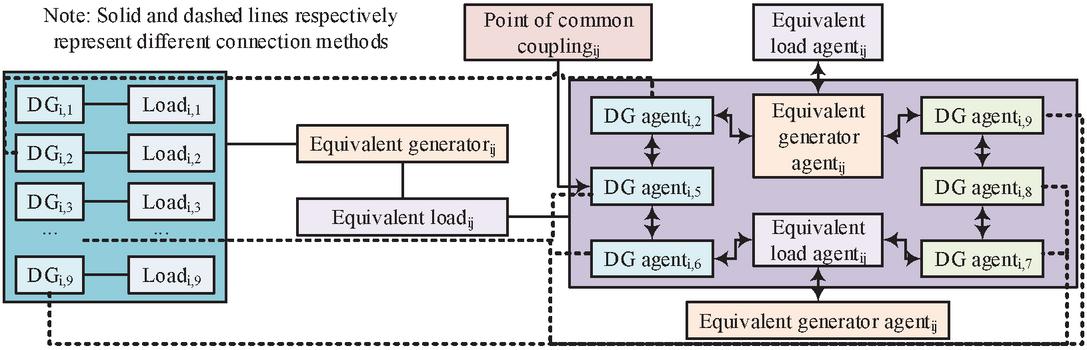
Figure 1 Double-layer optimization model on the power generation side.

In Figure 1, the double-layer optimization model on the power generation side collects power fluctuation information within the PG and the previous scheduling plan of adjacent micro-grids through common coupling point agents, EG agents, and EL agents, and optimizes the output of fossil fuel PGUs in the current PG in the upper layer information network. It is worth noting that the power fluctuation data transmitted through the common coupling point proxy has a critical impact on the access status of EGs and ELs [18]. Meanwhile, as the CE cost model belongs to a non-smooth step function, it needs to be approximated during the iterative solution process of the model. The solution formula is shown in Equation (19).

$$\{\begin{array}{c}{d}_{\mathit{MG},i}[k]=\rho d_{\mathit{MG},i}[k-1]+(1-\rho )W_{\mathit{MG},i}[k]\nabla {\tilde{S}}_{\mathit{MG},i}[k]\hfill \\ P_{\mathit{MG},i}[k+1]=P_{\mathit{MG},i}[k]+d_{\mathit{MG},i}[k]\hfill \\ p_{\mathit{MG},ij}[k+1]=\{\begin{array}{c}{p}_{\mathit{MG},ij,\min },p_{\mathit{MG},ij}[k+1]<p_{\mathit{MG},ij,\min }\hfill \\ p_{\mathit{MG},ij}[k+1],p_{\mathit{MG},ij,\min }\le p_{\mathit{MG},ij}[k+1]\hfill \\ \le p_{\mathit{MG},ij,\max }\hfill \\ P_{\mathit{MG},ij,\max },P_{\mathit{MG},ij}[k+1]>p_{\mathit{MG},ij,\max }\hfill \end{array}\hfill \end{array}$$

(19)

In Equation (19), $d_{\mathit{MG},i}[k]$ represents the momentum term at iteration $k$ on the power generation side. $\rho$ represents the inertia coefficient of the smooth momentum term. $W_{\mathit{MG},i}[k]$ represents the dynamic weight matrix when iterating $k$ times on the power generation side. $\nabla {\tilde{S}}_{\mathit{MG},i}[k]$ represents the sub-gradient when iterating $k$ times on the power generation side. $P_{\mathit{MG},i}[k]$ represents the power vector. $p_{\mathit{MG},ij,\max }$ and $p_{\mathit{MG},ij,\min }$ are the upper and lower limits of the constituent elements of the power vector, respectively. The resolution procedure of the double-layer optimization model on the power generation side is shown in Figure 2.

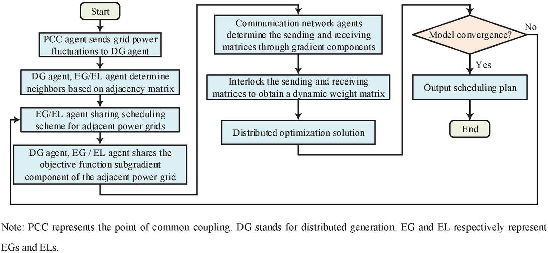
Figure 2 Resolution procedure of the two-layer optimization model on the power generation side.

In Figure 2, first, the power fluctuation information inside the PG is sent to the distributed power generation agent through the common coupling point agent, and the neighbors of the distributed power generation agent, EG agent, and EL agent are determined based on the adjacency matrix. Then, the EG agent and the EL agent are utilized to share the current dispatching scheme and sub-gradient components with the adjacent power generation (PG) units. Subsequently, the receiving and sending matrices within the communication network are determined. The above matrix is synchronized and locked to obtain a dynamic weight matrix [19, 20]. Then the distributed Eco-D model is solved. At this time, if the model meets the convergence condition, the dispatching scheme is output, otherwise the current dispatching scheme is shared with the adjacent PG again. For the demand side, its double-layer optimization model is shown in Figure 3.

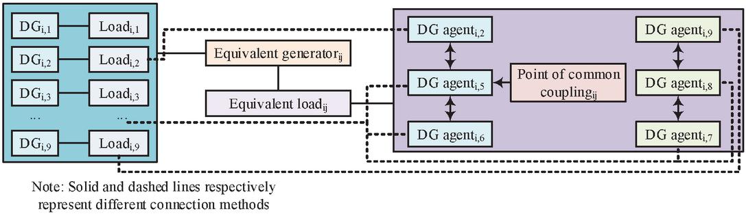
Figure 3 Double-layer optimization model on the demand side.

As depicted in Figure 3, the demand-side double-layer optimization model gathers information on the upcoming access volume and the time-of-use electricity price adjustment plan of the PG unit via a common coupling point proxy. Using this information, it optimizes the access volume of flexible loads through the information network. The solution formula for the double-layer optimization model on the demand side is shown in Equation (20).

$$\{\begin{array}{c}{d}_{\mathit{Load},i}[k]=\rho d_{\mathit{Load},i}[k-1]+(1-\rho )W_{\mathit{Load},i}[k]\nabla {\tilde{S}}_{\mathit{Load},i}[k]\hfill \\ L_i[k+1]=L_i[k]+d_{\mathit{Load},i}[k]\hfill \\ l_{ij}[k+1]=\{\begin{array}{c}0,l_{ij}[k+1]<0\hfill \\ l_{ij}[k+1],0\le l_{ij}[k+1]\le l_{ij,\max }\hfill \\ l_{ij,\max },l_{ij}[k+1]>l_{ij,\max }\hfill \end{array}\hfill \end{array}$$

(20)

In Equation (20), $d_{\mathit{Load},i}[k]$ represents the momentum term on the demand side. $W_{\mathit{Load},i}[k]$ represents the dynamic weight matrix on the demand side. $\nabla {\tilde{S}}_{\mathit{Load},i}[k]$ represents the sub-gradient on the demand side. $L_i[k+1]$ represents a vector composed of variables to be optimized. $l_{ij}[k+1]$ represents the elements in the variable vector to be optimized. $l_{ij,\max }$ and $l_{ij,\min }$ are the upper and lower limits of vector elements. The solution process of the demand side double-layer optimization model is shown in Figure 4.

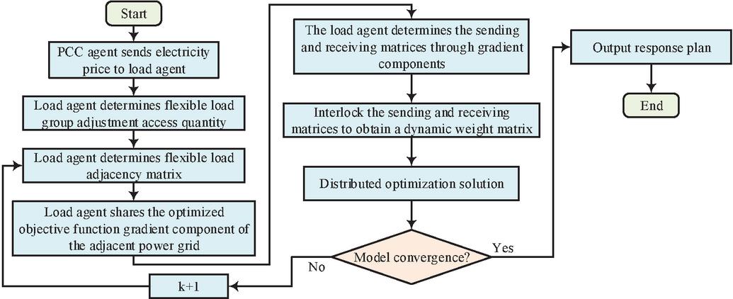
Figure 4 Resolution procedure of the demand-side double-layer optimization model.

In Figure 4, the time-of-use electricity price is first sent to the load agent through the common coupling point proxy. The load agent will adjust the flexible load group access volume at the corresponding time and determine its adjacency matrix. Then, the response optimization objective function gradient components of adjacent PGs are shared through load agents, and the receiving matrix and sending matrix are determined based on them. The model synchronizes and locks the above matrix to obtain a dynamic weight matrix. Finally, the model is solved, and if it satisfies the convergence condition, the response scheme is output. Otherwise, the gradient components of the response optimization objective function of the adjacent PG will be shared again.

3 Results

3.1 Simulation Environment Settings

To confirm the capability of the raised distributed optimization scheduling method for smart grids, simulation tests were conducted. The simulation testing platform was MATLAB/Simulink platform. In the simulation test, the factors of distributed power sources are given in Table 1.

Table 1 Distributed power supply factors

Distributed	Power	Fuel	Fuel	Fuel
Power	Rating	Quadratic	Primary	Constant
Supply	(kW)	Term Coefficient	Term Coefficient	Term Coefficient
1-1	280	/	/	/
1-2	5500	0.06	6.42	79.03
1-3	5000	0.07	5.21	79.96
1-4	260	/	/	/
1-5	4000	0.07	6.08	70.05
2-1	230	/	/	/
2-2	7000	0.07	6.03	69.99
2-3	200	/	/	/
2-4	290	/	/	/
2-5	6000	0.08	5.82	64.21
3-1	290	/	/	/
3-2	5500	0.06	5.28	69.21
3-3	90	/	/	/
3-4	200	/	/	/
3-5	5000	0.06	6.20	82.08

According to Table 1, distributed power sources 1-1, 1-4, 2-1, 2-3, 2-4, 3-1, 3-3, and 3-4 were all renewable energy generators, while the rest were fossil fuel generators. For fossil fuel generators, their carbon quota factor and CE factor were 0.41 kg/kWh and 0.65 kg/kWh, respectively. For renewable energy generators, the additional marginal carbon quota factor was 0.05 kg/kWh. The starting and trading prices for CE costs were 0.27 Chinese Yuan (CNY)/kg and 0.41 CNY/kg, respectively. The length of the CE interval and the cost increase were 20 kg and 1, respectively. The power exchange and load parameters are given in Table 2.

Table 2 Power exchange and load parameters

PG	PG 1	PG 2	PG 3
PG 1	/	0.48	0.49
PG 2	0.51	/	0.45
PG 3	0.45	0.46	/
Load	Load requirements	Quadratic term coefficients of the utility function	Utility function once the term coefficient
1-1	0–6550	2.01	0.04
1-2	2000	/	/
1-3	260	/	/
1-4	0–660	2.60	0.04
1-5	2000	/	/
2-1	100	/	/
2-2	0–2550	2.37	0.04
2-3	0–2100	2.71	0.04
2-4	0–2500	2.83	0.03
2-5	1550	/	/
3-1	0–350	2.19	0.04
3-2	0–2550	2.57	0.04
3-3	2550	/	/
3-4	0–3530	2.03	0.05
3-5	2500	/	/

According to Table 2, the power exchange coefficients between PGs were all between 0.45–0.51, and the quadratic coefficients of each load utility function were above 2.0, while the first-order coefficients were generally around 0.04. During testing, the line voltage and system frequency of the PG were 380 V and 50 Hz, respectively, and the impedance of the transmission line per 1 km was 0.64+j0.1 ohms. In addition, to obtain input scenarios for simulation testing, the study utilized Latin hypercube sampling to process the data and reduced it using K-means. The wind and photovoltaic power of typical scenarios are shown in Figure 5.

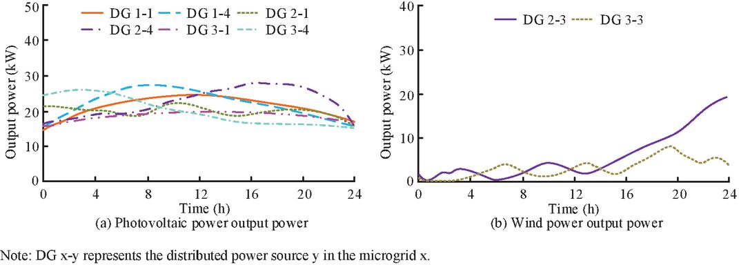
Figure 5 Wind power and photovoltaic power in a typical scenario.

As shown in Figure 5(a), the output power (OP) of photovoltaic power sources varied significantly within 24 hours, but the minimum OP of all photovoltaic power sources was around 5 kV. As shown in Figure 5(b), the OP of the wind PGU gradually increased over time, and the OP of DG2-3 and DG3-3 both significantly increased after 16:00.

3.2 Analysis of Load and Environmental Fluctuations Impact

The study first investigated the scheduling results of the proposed distributed optimization method when both load and environment fluctuated. The OP of fossil fuel power sources in each PG is shown in Figure 6.

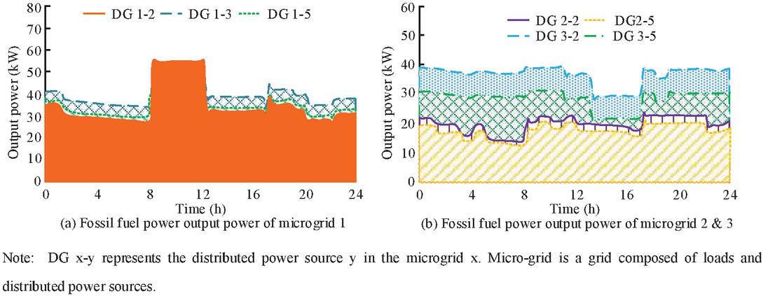
Figure 6 Output Power (OP) of the fossil fuel power supply.

According to Figure 6(a), in smart micro-grid 1, the OP trends of various fossil fuel power sources were basically consistent, reaching their maximum within the range of 8–12 hrs. The maximum OP of DG 1-2, DG 1-3, and DG 1-5 were 56 kW, 52 kW, and 45 kW, respectively. According to Figure 6(b), in smart micro-grids 2 and 3, the OP variation trend of fossil fuel power sources in the same grid was consistent. The OP of the fossil fuel power source in micro-grid 2 reached its minimum at 8 hrs, while micro-grid 3 reached its minimum between 13 and 17 hrs. After the distributed optimization method proposed through research scheduling, each micro-grid could flexibly adjust its OP. The incremental cost of fossil fuel power sources for each PG is shown in Figure 7.

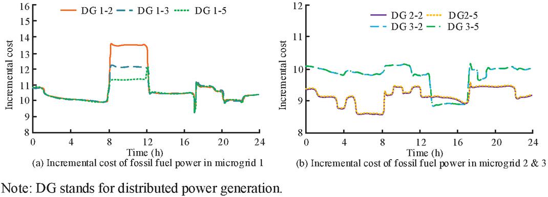
Figure 7 Incremental cost of fossil fuel power supply.

As shown in Figure 7(a), the incremental cost trend of each fossil fuel power source in smart micro-grid 1 was consistent. Among them, DG 1-2 had the highest incremental cost, which could reach up to 13.8. DG 1-5 had the smallest incremental cost, with a maximum incremental cost of only 12.2. As shown in Figure 7(b), the incremental cost of fossil fuel power sources in the same grid was consistent in smart micro-grids 2 and 3. The minimum incremental costs of the two were 8.5 and 8.7, and the maximum were 9.6 and 10.2, respectively. The above results indicated that after the proposed distributed optimization method for scheduling, each micro-grid could maintain the consistency of its incremental cost, that is, each grid achieved optimal economic scheduling.

3.3 Demand Side Response Impact and CE Cost Analysis

To confirm the impact of the demand side effects on the interests of users, a simulation test without considering the demand response was conducted, and the optimization effect of the micro-grid with different loads and distributed power supply was compared. The flexible load access of each PG is shown in Figure 8.

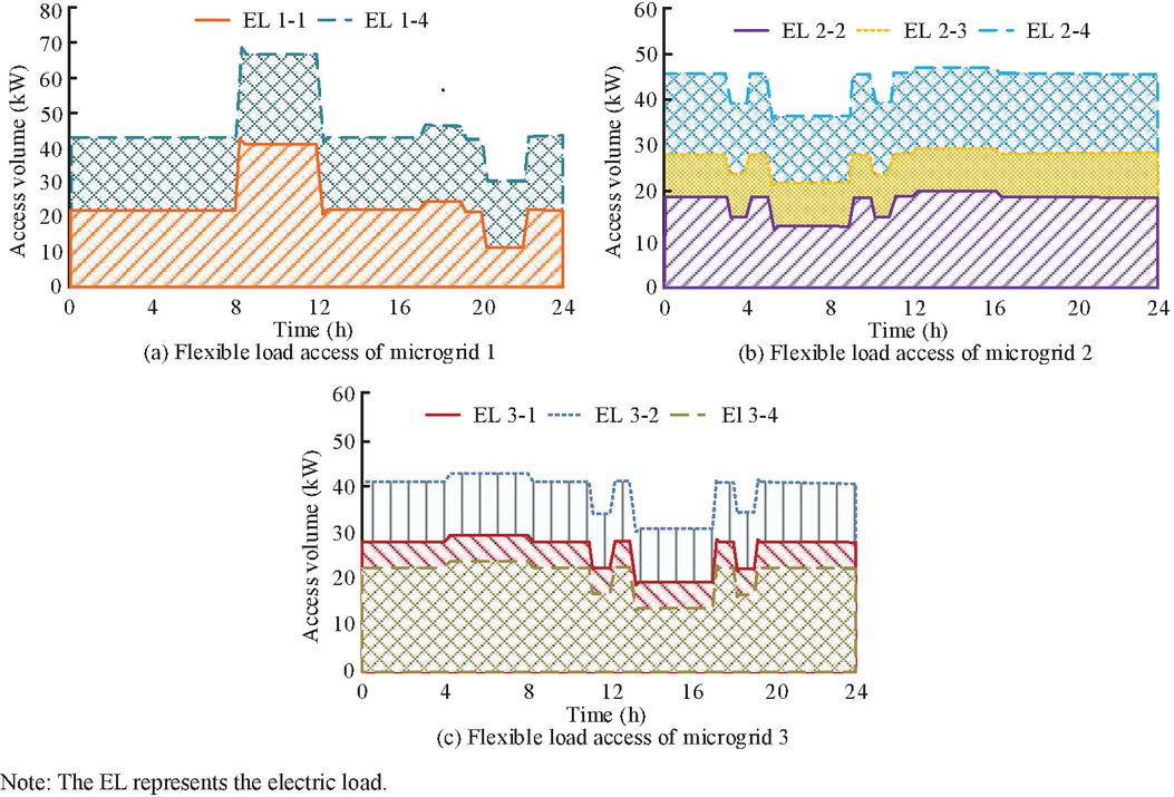
Figure 8 Flexible load access volume.

As shown in Figure 8(a), the trend of flexible load integration in micro-grid 1 was completely consistent. The flexible load connection amount of EL 1-1 was always lower than that of EL 1-4, and the connection amounts of both reached their peak between 8 and 12 hrs, which was consistent with the OP changes of distributed power sources in its PG 1. In Figure 8 (b), the trend of flexible load access in micro-grid 2 was consistent. Among them, EL 2-4 had the highest access volume, and all three showed significant fluctuations between 3 and 12 hrs. As shown in Figure 8(c), the trend of flexible load access in micro-grid 3 was also consistent, with significant fluctuations between 11 and 19 hrs for all three micro-grids. The user-side revenue situation is shown in Figure 9.

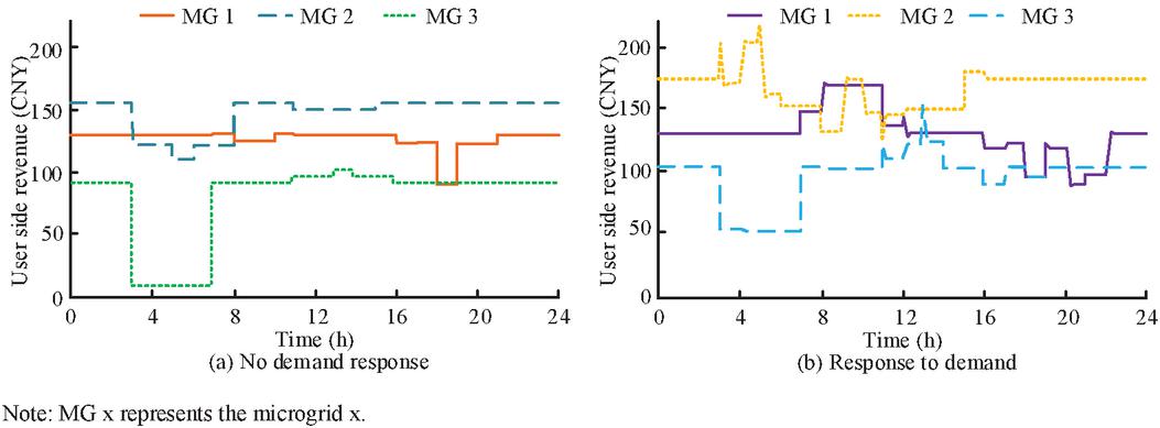
Figure 9 User-side revenue situation.

Comparing Figures 9(a) and 9(b), compared to the situation without demand response, the user side benefits significantly increased under the condition of demand response. Among them, micro-grid 1 had the highest user side revenue of 125 CNY and 175 CNY respectively in the absence/presence of demand response. The highest user side revenue for micro-grid 2 in the absence/presence of demand response was 153 CNY and 224 CNY, respectively. The highest user side benefits for micro-grid 3 in the absence/presence of demand response were 100 CNY and 150 CNY, respectively. The user side revenue of the three increased by 40%, 46%, and 50% respectively. The above results indicated that the proposed distributed optimization method for PG Eco-D could effectively improve user side benefits. The CE cost of micro-grids is shown in Figure 10.

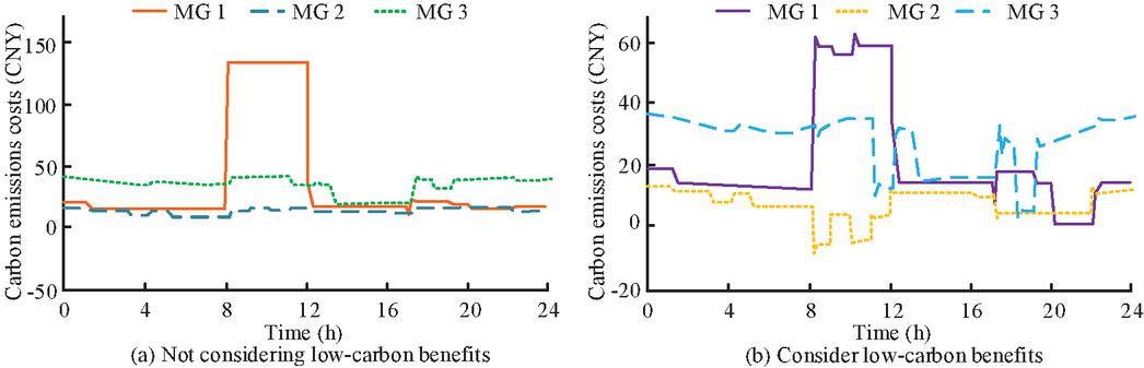
Figure 10 CE costs of micro-grids.

Comparing Figures 10(a) and 10(b), after considering low-carbon benefits, the CE costs of each micro-grid were significantly reduced. Without considering the CE benefits, the highest CE costs for micro-grids 1, 2, and 3 were 137 CNY, 13 CNY, and 45 CNY, respectively. Considering the CE benefits, the highest CE costs for micro-grids 1, 2, and 3 were 62 CNY, 11 CNY, and 38 CNY, respectively, reducing them by 55%, 16%, and 16%, respectively. The above results indicated that the proposed distributed optimization method for PG Eco-D could effectively reduce CE costs.

4 Discussion and Conclusion

To achieve Eco-D of multi-intelligent micro-grids, a distributed optimization model for Eco-D of smart grids was proposed, and its effectiveness in improving user side benefits and reducing CE costs was verified through simulation testing. The test results showed that considering demand response, for micro-grids 1, 2, and 3 with different distributed power sources and loads, their user-side revenue increased by 40%, 46%, and 50%, respectively, which was significantly better than the situation without demand response. Meanwhile, considering low-carbon benefits, the CE costs of each micro-grid significantly decreased, with micro-grids 1, 2, and 3 reducing their CE costs by 55%, 16%, and 16%, respectively. This was because the proposed Eco-D model for the PG could achieve dual interaction of PG information and energy, and fully considered the power exchange problem between PGs, enabling it to achieve dual-layer scheduling between networks, validly curbing the cost of micro-grids and raising the economic benefits of users. The above results indicated that the proposed model had the potential to achieve a win-win situation of economic and environmental benefits, providing an effective solution for the Eco-D of smart grids. However, due to the absence of the effects of energy storage units on the PG when constructing Eco-D models, the model had poor dispatch performance when facing power systems with energy storage units. Therefore, in the future, energy storage units will be introduced into the model to enhance the renewable energy consumption rate of the PG.

References

[1] Wang Z, Wang D, Wen C, and Wang, W. “Push-Based Distributed Economic Dispatch in Smart Grids Over Time-Varying Unbalanced Directed Graphs”. IEEE Transactions on Smart Grid, 2021, 12(4): 3185–3199.

[2] Dong W, Yang Q, Li W, and Zomaya, A. Y. “Machine-Learning-Based Real-Time Economic Dispatch in Islanding Microgrids in a Cloud-Edge Computing Environment”. IEEE Internet of Things Journal, 2021, 8(17): 13703–13711.

[3] Navas F A, Gomez J S, Llanos J, Rute E, and Sumner M. “Distributed Predictive Control Strategy for Frequency Restoration of Microgrids Considering Optimal Dispatch”. IEEE Transactions on Smart Grid, 2021, 12(4): 2748–2759.

[4] Yuan Z P, Xia J, Li P. “Two-Time-Scale Energy Management for Microgrids with Data-Based Day-Ahead Distributionally Robust Chance-Constrained Scheduling”. IEEE Transactions on Smart Grid, 2021, 12(6): 4778–4787.

[5] Saeed M H, Rana M D S, Kausaraahmed M. D. El-Bayeh Claude ZiadFangzong, Wang. “Demand response based microgrid’s economic dispatch”. International Journal of Renewable Energy Development, 2023, 12(4): 749–759.

[6] Basu M, Jena C, Khan B, and Ali, A. “Optimal Bidding Strategies of Microgrid with Demand Side Management for Economic Emission Dispatch Incorporating Uncertainty and Outage of Renewable Energy Sources”. Energy Engineering, 2024, 121(4): 849–867.

[7] Minor-Popocatl H, Omar Aguilar-Mejía, Francisco Daniel Santillán-Lemus, Valderrabano-Gonzalez A, and Samper-Torres R I. “Economic dispatch in micro-grids with alternative energy sources and batteries”. Latin America Transactions, 2023, 21(1): 124–132.

[8] Zhou Y, Zhai Q, Wu L. “Optimal Operation of Regional Microgrids with Renewable and Energy Storage: Solution Robustness and Nonanticipativity Against Uncertainties”. IEEE Transactions on Smart Grid, 2022, 13(6): 4218–4230.

[9] Moazeni F, Khazaei J, Asrari A. “Step Towards Energy-Water Smart Microgrids; Buildings Thermal Energy and Water Demand Management Embedded in Economic Dispatch”. IEEE Transactions on Smart Grid, 2021, 12(5): 3680–3691.

[10] Dey B, Basak S, Bhattacharyya B. “Demand-Side-Management-Based Bi-level Intelligent Optimal Approach for Cost-Centric Energy Management of a Microgrid System”. Arabian Journal for Science and Engineering, 2023, 48(5): 6819–6830.

[11] Yang Y D, Qiu J L, Qin Z J. “Multidimensional Firefly Algorithm for Solving Day-Ahead Scheduling Optimization in Microgrid”. Journal of Electrical Engineering and Technology, 2021, 16(4): 1755–1768.

[12] Islam M M, Nagrial M, Rizk J, and Hellany A. “Dual stage microgrid energy resource optimization strategy considering renewable and battery storage systems”. International Journal of Energy Research, 2021, 45(15): 21340–21364.

[13] Ghaderyan D, Pereira F L, Aguiar A P. “A fully distributed method for distributed multiagent system in a microgrid”. Energy Reports, 2021, 7(5): 2294–2301.

[14] Kurundkar K M, Vaidya G A. “Voltage Control Ancillary Service Through Grid-Connected Microgrid, Its Pricing by Optimized Active Power and Reactive Power Management Using IEHO-TOPSIS Approach”. Iranian Journal of Science and Technology, Transactions of Electrical Engineering, 2024, 48(1): 229–250.

[15] Samimi A, Shateri H. “Network constrained optimal performance of DER and CHP based micro-grids within an integrated active-reactive and heat powers scheduling”. Ain Shams Engineering Journal, 2021, 12(4): 3819–3834.

[16] Bhattacharya A B, Singh M. “Performance analysis of adaptive smart controllers for islanded microgrid”. International journal of emerging electric power systems, 2022, 23(3): 391–408.

[17] Tseng C J, Dwijendra N K A, Opulencia S M I. “Optimal Energy Management in a Smart Micro Grid with Demand Side Participation”. Environmental and Climate Technologies, 2022, 26(1): 228–239.

[18] Bastawy M, Ebeed M, Kamel K S. “Optimal day-ahead scheduling in micro-grid with renewable based DGs and smart charging station of EVs using an enhanced manta-ray foraging optimisation”. IET Renewable Power Generation, 2022, 16(11): 2413–2428.

[19] Yuan G, Xie F. “Digital Twin-Based economic assessment of solar energy in smart microgrids using reinforcement learning technique”. Solar Energy, 2023, 250(1): 398–408.

Biographies

Jinlin Chen graduated from Hunan University of Technology in 2019, obtaining a master’s degree in electrical engineering. At present, he is a teacher at Henan Polytechnic Institute, his main research directions are new energy power generation and intelligent control.

Nianwei Hu received her BE in electronic information technology from South-Central Minzu University in 2016. She received her ME in detection technology and automation from Beijing University of Civil Engineering and Architecture in 2019. Presently, she is working as a full-time teacher at Henan Polytechnic Institute. Her areas of interest are electrical engineering, intelligent control, industrial robotics, etc.

Distributed Generation & Alternative Energy Journal, Vol. 40_3, 457–480.
doi: 10.13052/dgaej2156-3306.4031
© 2025 River Publishers