Decision-Making Method for County Power Grid Dispatching with High Proportion of Renewable Energy
Chao Wang1, Yuan Niu1,*, Lei Zuo2, Rui Yu3, Gaohua Liu3 and Zhijun E2
1Ninghe Power Supply Branch of State Grid Tianjin Electric Power Company, State Grid Tianjin Electric Power, Tianjin, 301500, China
2State Grid Tianjin Electric Power Company, Tianjin, 300010, China
3School of Electrical and Information Engineering, Tianjin University, Tianjin 300072, China
E-mail: yyrr2024_2096@tju.edu.cn
*Corresponding Author
Received 02 May 2025; Accepted 28 May 2025
Abstract
With the continuous increase in the proportion of new energy integrated into rural distribution networks, numerous challenges emerge in its dispatching decision-making. This study focuses on this issue and aims to propose an innovative hierarchical regulation method for the maximum and minimum thresholds of new energy with reserve included, so as to achieve efficient dispatching of county power grids. Facing issues like inadequate investment and chaotic management in current county distribution networks, and the lack of market impact consideration in existing research, the paper first analyzes the dispatching decision-making structure involving elastic resources and control strategies. It then introduces the interactive dispatching mechanism with concepts of load aggregators and source attributes. The core hierarchical regulation method covers data preprocessing, cost objective function establishment, and dispatching decision-making. Case studies using actual grid data analyze factors affecting new energy reserve ratio. The developed cloud-edge-end collaborative model with demand-side management realizes multi-time-scale rolling dispatching, reducing new energy volatility and grid operation costs, thus providing an effective solution for high-proportion new energy integration in county power grids.
Keywords: County power system, decision-making method, dispatching, hierarchical regulation, particle swarm optimization algorithm.
1 Introduction
The distribution network has far more equipment than the leading network, and its complexity, perception accuracy, and scheduling management difficulties are far beyond the leading network [1, 2]. Due to historical reasons, some county distribution networks in China face issues such as insufficient investment, unclear asset division, lengthy fault processing, and ambiguous scheduling responsibilities. Consequently, distribution network scheduling and operation management in many areas remain in a lax ’invisible, untouchable, uncontrollable’ mode. The lack of standards for dispatching regulation further hinders its development and implementation [3, 4].
Considering demand-side resources simultaneously with economic dispatch on the generation side is critical to achieving high-proportion access to new energy (NE) to the distribution network. The demand response policy is rationally formulated through practical measures to encourage users to participate in load-side carbon emission management. Gao et al. conduct demand-side management of power users based on marginal carbon emission intensity. The upper layer is a multi-objective optimization framework for the power system, targeting the objectives of minimizing generation cost and carbon emissions, and the lower layer is a load-side optimization model considering load satisfaction. The above constructs a household electricity management model considering electricity price and carbon emission intensity and conducts load management based on multi-objective optimization. However, it pays less attention to the influence of market implementation on the power system scheduling strategy [5, 6].
The introduction of the concept of low-carbon electricity has offered new perspectives on the traditional day-ahead scheduling problem. The carbon trading market mechanism and carbon emission prices is crucial for day-ahead scheduling. Active distribution grids (ADN) integrate multiple demand-side resources. The distributed power sources within them are mostly gas, oil, or renewable energy sources with low carbon emissions [7]. Studying the impact of active distribution grids on the carbon emissions of transmission grids can fully utilize the low-emission characteristics of active distribution grids and relieve the carbon-emission pressure on transmission grids. A study establishes a coordinated scheduling framework for a power system incorporating interactive loads [8]. The optimization objectives, including minimum operating cost and network loss, are solved by fuzzy methods. High-energy-carrying loads participate in the optimal scheduling of the power system [9]. A model for optimizing the accommodation of wind power and minimizing the system’s operating cost has been developed. High-energy-carrying loads accommodate the fluctuating nature of wind power. Many studies transform this problem into a two-layer model for a solution. The upper-layer model determines the output of conventional and wind power sources, while the lower-layer model enables the effective participation of high-energy-carrying loads. The two-layer model is solved by a hybrid algorithm combining the improved genetic algorithm (GA) and binary particle swarm optimization algorithm (PSO).
Existing studies provide methodological foundations for source-load coordination optimization, model construction, and algorithm application, but they generally suffer from limitations such as insufficient scenario adaptability, single-dimensional resource integration, and lack of reserve and market mechanisms. Meanwhile, addressing issues like grid integration barriers and increased network losses caused by large-scale new energy grid connection, measures such as deploying energy storage, expanding consumption areas, and involving electric vehicles in scheduling can effectively mitigate the negative impacts of new energy integration. Thus, this paper proposes a dispatch decision-making method for high-proportion new energy integration into rural distribution networks through innovations including hierarchical regulation frameworks, multi-resource aggregation, multi-time-scale coordination, and market mechanism integration. By deploying electric vehicles and energy storage systems and establishing a cluster control model, the method enhances scheduling flexibility and mitigates the impacts of new energy grid integration. This not only fills the research gap in high-proportion new energy dispatch scenarios for county-level distribution networks but also provides more practicable solutions to address the real-world challenges of county power grids under dual-carbon goals.
2 Organizational Structure for Distribution Network Dispatch Decision-Making
2.1 Elastic Resources of Various Types
Guiding the participation of load-side elastic resources in power grid demand response requires research from market and distribution network physical topology. Guiding the participation of load-side elastic resources in power grid demand response requires research from market and distribution network physical topology. In the electricity trading market, the types of electricity users who can participate in grid demand response mainly include residential, industrial, and commercial users. Among them, the characteristics of residential users include the massive size of residents, low individual electricity consumption, and significant differences in the willingness of different residents to respond to power grid regulations [10]. Industrial users are the leading players in the high-load electricity market, and their elastic load resources are closely related to their own generated products. Generally, industrial users have a large elastic capacity to schedule loads. Still, there are specific characteristics of insufficient flexibility in load adjustment periods, power, and certainty (mainly influenced by production orders). However, they cannot be ignored as critical elastic resources on the load side. Commercial users’ electricity consumption and flexibility are between residential and industrial users, and their electricity consumption is relatively high, low in quantity, and low in flexibility compared to individual residential users [11]. Compared to industrial users, commercial users have a more significant number, lower electricity consumption, and higher flexibility and autonomy in adjustment [12]. The elastic resources of various market entities are shown in Table 1. There are significant differences in residential electricity consumption, commercial supporting facilities, and industrial industries on the distribution side in different regions of China, resulting in substantial variations in the adjustable load resources of various market entities in different areas.
Table 1 List of elastic resources of various types in market entities
| Energy Storage | Class of Energy | Transferable | Basic | |
| Load Type | Equipment | Storage Devices | Load Equipment | Load Equipment |
| Residential users | Distributed generation supporting storage system, etc | Air conditioning, refrigerator, heater, electric vehicle, etc | Washing machine, disinfection cabinet, TV, etc | Lighting, range hood, rice cooker, etc |
| Industrial user | Self-storage battery, etc | Air conditioning, cold storage, electric cars, etc | Non-essential production peripherals | Core product manufacturing equipment |
| Business user | Self-storage battery, etc | Air conditioning, freezers, fresh air systems, electric vehicles, etc | Non-essential commercial peripherals | Core business operation equipment |
2.2 Scheduling Control Strategy Approach
On the power generation side of the active distribution network, clean energy sources including wind turbines and solar panels can be integrated. Meanwhile, on the load consumption side, adjustable loads such as energy storage devices and electric vehicles can be connected [13]. When operators conduct optimization scheduling, they start from the NE output power on the power generation side and the adjustable load on the load consumption side simultaneously. This coordinated approach enables the active distribution network to have stronger flexibility and higher capacity for NE consumption, which is an advanced stage in developing the distribution network [14]. Through advanced technologies and control strategies, active distribution networks coordinate and manage equipment, including the power output of solar and wind generation, energy storage devices, and electric vehicles. This enables an improvement in the new-energy accommodation capacity and a reduction in operating costs while ensuring safety.
The distribution network’s intelligent scheduling mode realizes the intelligent distribution supply operation management. The distribution network management system utilizes satellite detection technology and GPS to conduct spatial detection of distribution resources, enabling coordination among the distribution network management system, power supply, and current supply load regulation. The power supply conducts intelligent power supply based on the prediction results of distribution forecasting technology. The system detects the intensity of transmitted current through satellite detection technology and then intelligently adjusts the amount of current transmission. Finally, the distribution operation network management system conducts intelligent inspection using the feedback data from the GPS-positioned system to complete the operation of the matching-point mode. Under the centralized control strategy, the control center shoulders the task of controlling each load to participate in demand response. The control center monitors the system frequency deviation. Then, it calculates the target of load adjustment and sends the control signals to a large number of dynamically controllable loads one by one. The control center establishes a two-way communication network with each device and collects the operating status of the devices while sending out control signals. Depending on how demand response is achieved and how communication is transmitted, control strategies for adjustable load resources are broadly categorized into three types: centralized control, decentralized control, and hybrid control.
The centralized control strategy, as described above, has a high-level control center with great power, which can formulate complex load control strategies by considering all the factors and realizing the mutual communication of information with the power department. Figure 1 shows the operation frame of a typical centralized control strategy.
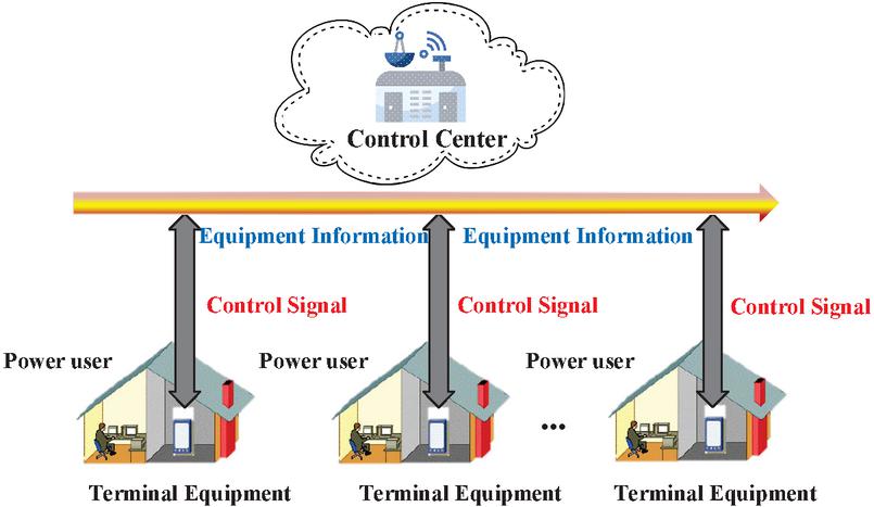
Figure 1 Schematic diagram of a typical centralized control strategy approach.
3 Implementation Mechanisms for Interactive Scheduling of County Distribution Networks
With the development of the electricity market, a new specialized entity, the load aggregator (LA), has emerged to serve as a coordinator between small customers and the system operator. Load aggregators are tasked with integrating demand-response resources on the user side and making them accessible to purchasers in the electricity market. Load aggregators can not only offer small and medium sized loads complex energy-service analysis and energy-saving guidance through data-mining and other technologies, but also aggregate a certain proportion of dynamically controllable loads to participate in the electricity market.
3.1 Concept of Load Aggregator
As the number of dynamically controllable loads is gradually increasing, more attention is being paid to the resilience and flexibility of the load side, and load aggregators are emerging [15]. As a bridge between a large number of decentralized loads and the system operator, they diversify the power system regulation resources, thus enabling the realization of the potential of dynamically controllable loads. Overseas research on load aggregators began earlier, initially defining this intermediary between operators and customers as ’load service entities’ (LSE). LSE later expanded beyond electricity trading to evolve into load aggregators, specializing in customer demand-response services. Load aggregators initially carried out demand-response work for large industrial and commercial customers, whose response greatly impacted the entire grid operation, and the work was relatively simple. However, with the smart grid’s advancement, the scale of demand-side management is gradually expanding. Users of small and medium size also possess the potential to participate in the electricity trading market. For users of small and medium size, the influence of individual loads is very small, not meeting the standard for participating in the power market. So load aggregators must play a bridging role, using regulatory means to aggregate small and medium sized loads into a whole. Domestic research on load aggregators was initiated relatively late. Load aggregators are responsible for evaluating the potential for customer participation in demand response, integrating scattered demand-response resources through a series of technical means, and so contributing to the power system’s functioning. Currently, load aggregators and similar entities in China are still in the initial stage. But with the development of China’s reform on the electric power system, the market-oriented operation is constantly being perfected during the reform, and the research on aggregation technology for small and medium sized users and the demand-response model based on load aggregators meets the needs of development.
From a power system operations perspective, a load aggregator is a third-party organization used to integrate demand response resource individuals (loads or energy storage devices) and thus participate in market-based and non-market-based demand response activities on behalf of those individuals. Its profitability is primarily based on selling the demand response services it provides in the marketplace. Broadly speaking, the load aggregator’s demand response resources are not limited to traditional electric loads, but can also include distributed generating units such as wind and solar [16]. These units can provide system stabilization services to the distribution company or directly to the transmission system operator. The load aggregator’s participation in scheduling in the distribution network is illustrated schematically in Figure 2.
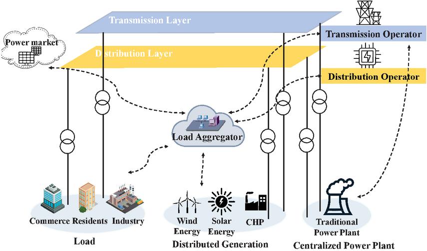
Figure 2 Schematic diagram of load aggregator participation in scheduling in the distribution network.
From the user’s perspective, the load aggregator functions similarly to an energy service provider. It analyzes the energy-usage characteristics of users within its purview, evaluates their capacity to take part in demand response, and guides users to employ energy intelligently. This is achieved through technical means like data mining, user profiling, and social methods such as questionnaire surveys. Users’ benefits mainly consist of electricity-saving gains and profits from participating in demand response by signing contracts with load aggregators.
3.2 Source Property
In contrast to the traditional distribution network, the active engagement on the “source” part and the positive response of the active distribution network’s demand part enable the original distribution network to transform from passive processing to active consumption, with its “active” core being more prominent [17, 18]. This makes the control variables, constraints, and objective function more complicated. The active distribution grid is a system of active control and active regulation on the “source-load” side. It fully realizes the potential of the active role of regulatable resources such as distributed power generation, distributed energy storage facilities, and the loads with demand side response characteristics in the planning and operation of power grids, ensuring the optimal integration of resources across the grid, optimizes the proportion of renewable energy utilization, and improves the utilization rate of smart grids, to ensure the secure and dependable operation of the grid while maximizing the grid utilization rate. The optimal scheduling of the active distribution network involves rational and optimal control in three aspects, namely power source, network, and flexible load, to enhance the capacity of renewable energy consumption, achieve energy-saving and loss-reduction, and make the operation of the power grid safer and more reliable. This chapter analyzes the physical principles of different types of distributed power sources (controllable and uncontrollable units) as well as the output characteristics of each distributed unit. On the “load” side, this chapter analyzes the working principles of energy storage units, flexible loads, and electric vehicles. For flexible loads, corresponding constraints are given according to their different working characteristics.
4 Hierarchical Approach to Regulating the Maximum and Minimum Values of New Energy Sources for Incorporation into Backups
Optimized scheduling research should first clarify the relationship between asset attribution and interest. This paper assumes that all kinds of distributed generation (DG) and microgrids belong to users, while energy storage devices are invested and constructed by the grid company. The grid company gives revenue from DG to users, but DG should obey grid scheduling. Microgrids conduct two-way electricity trading with the active distribution network (ADN), but they need to report the power plan of the point of common coupling (PCC) to the control center daily and accept the scheduling. Moreover, users who accept the demand side management (DSM) can get economic compensation for load shedding and leveling. To promote green power consumption, the power curtailment of wind and solar DG is not considered at the time.
4.1 Pre-processing for Data Acquisition and Correlation
Obtain historical meteorological data. Also, acquire historical three-month county-wide distributed wind turbine and photovoltaic generation data, along with load data from user-side smart meter statistics. The Pearson correlation coefficient and multiple linear regression are used to analyze correlations between factors influencing power generation or load data, enabling specific day-ahead predictions [19, 20].
Retrieve historical three-month meteorological data, distributed wind power generation data, and user-side load data from the energy management system (EMS). The correlation between two data sets can be expressed by the Pearson correlation coefficient. Pre-process the data by numbering the data points chronologically, and Table 2 shows the data processing forms.
| Photovoltaic | Wind | ||||||
| Date | Power | Power | User | Humidity | Light | ||
| Type | Generation | Generation | Load | Temp | Level | … | Intensity |
| Number | Y | Y | Y | X | X | … | X |
The obtained X to X data in one year were averaged with Y, Y, and Y data, respectively, and brought in:
| (1) |
Where, represents the -th observed value of variable ; is the mean of variable ; represents the -th observed value of variable ; is the mean of variable ; and is the sample size. This formula is used to measure the degree of linear correlation between variable and variable .
Calculate the r-value, which represents the correlation between the two variables, x and y. Judge the calculated value as follows:
• When , it can be regarded as a high-degree correlation;
• When , it can be considered a substantial correlation;
• When , it can be regarded as a practical correlation.
• When , it indicates that the relationship between the two variables is not apparent and can be regarded as a non-linear correlation.
Bring the data with a correlation greater than 0.3 into the multiple linear regression equation to predict the total amount of power generation and consumption on the previous day.
| (2) |
Where, is the predicted value, which is the prediction result of the independent variables obtained through the multiple linear regression model. is the intercept, reflecting the basic predicted value when all independent variables are zero. are the regression coefficients, representing the degree of influence of the independent variables on the predicted value . are the independent variables. In this paper, they are the influencing factors related to power generation or load data, such as temperature, humidity, etc. The total amount of day-ahead power generation and electricity consumption is predicted through the linear combination of these independent variables.
Use the obtained correlation coefficient to perform intraday hourly data statistics on the impact volume data with an absolute value of Pearson’s correlation coefficient data more significant than 0.3 and the household load data uploaded by the smart meter during the previous hour.
Enter the compliance data obtained from the intelligent terminal and the forecast data received from the edge IoT agent into the cloud platform, and then re-run the correlation coefficient calculation. Update the coefficient calculation, redo the hourly forecast, and input the results to the cloud computer at the master control station. The results are automatically updated to override the next hourly data forecast.
Input conventional constraint data to the computer, including generation constraints, battery charge level constraints, and transmission power constraint data.
Forecast the total value of power generation and consumption data, and update the total power balance constraints and supply and demand balance constraints data.
| (3) | |
| (4) |
Where, represents the total power of the system at time t. denotes the power generated by renewable energy sources at time t, such as that from distributed photovoltaic power generation, wind power generation and other renewable energy sources at this moment. represents the power sold to the conventional power grid at time t, stands for the power of the energy storage device at time t, and represents the power purchased from the conventional power grid at time t. This constraint indicates that the system is in a state of drawing power from the grid at this time.
4.2 Establishment of Objective Functions for Cost Decision Variables
Firstly, the size of distributed wind-generating units in the county is counted. Secondly, the sizes of distributed photovoltaic-generating units and energy-storage batteries in the county are also counted. Additionally, data related to other cost-related items, such as the cost of different types of equipment in the distribution network, are collected. The prices can be adjusted according to the specific models used in the county. Table 3 shows data sheets for various pollutant emissions related to green energy and carbon-emission costs. The calculation of distributed power generation based on Table 4 is combined with the following equation to calculate the required operating cost.
| (5) |
Where, represents the minimum value of the overall operating cost of distributed power sources, which is the target value of this cost-calculation model. denotes the unit electricity cost of the i-th type of distributed power source equipment, and represents the power generation of the i -th type of distributed power source equipment at time t. By multiplying the power generation of equipment of different types at different times by their corresponding unit electricity costs and then summing them up, the overall operating cost of distributed power sources is finally obtained.
Table 3 Costs of various kinds of equipment in the distribution network
| Power Generation | Electricity | |
| Equipment Type | Scale/kw | Cost/Yuan(kWh) |
| Photovoltaic Generator Set | 11000 | 0.851.30 |
| Wind Turbine Generator Set | 202000 | 0.450.97 |
| Fuel Cell | 52000 | 0.650.97 |
Table 4 Data sheet on emissions of various pollutants
| Pollutants(g/kwh) | NO | CO | CO | SO |
| PV (g/kwh) | 0 | 0 | 0 | 0 |
| Wind Power (g/kwh) | 0 | 0 | 0 | 0 |
| Fuel cell (g/kwh) | 0.022 | 635.04 | 0.0544 | 0 |
| Accumulators (g/kwh) | 0 | 0 | 0 | 0 |
The objective function for the county grid environment is constructed as follows:
| (6) |
Where, represents the minimum value of the environmental objective function of the county-level power grid. m represents the type of pollutant. is the weight coefficient of the m-th type of pollutant, which is used to measure the relative importance of each type of pollutant in the overall environmental objective function. represents the environmental impact amount or cost related to the m-th type of pollutant generated by the i-th type of distributed power source equipment at time t. Multiplying it by the power generation of this equipment at time t gives the environmental-impact-related number caused by the generation of a specific pollutant by this equipment at a specific time. represents the environmental impact amount or cost related to the m-th type of pollutant associated with the conventional power grid at time t. Multiplying it by the power obtained from the conventional power grid gives the environmental- impact-related value caused by the power-grid-related activities generating a specific pollutant at a specific time.
Input the statistical battery power supply data of the updated hourly forecast into the formula for battery life loss cost:
| (7) |
Where, represents the minimum value of the battery life-loss cost. denotes the coefficient of the battery life-loss cost, and represents the state parameter of the battery at time t. This parameter is related to factors such as the charge-discharge amount and state-of-charge of the battery.
Input the power purchase data from the superior power grid into the formula to calculate the power purchase cost of the power grid at the level above the county-level power grid:
| (8) | |
| (9) |
Where, represents the minimum value of the cost of purchasing electricity from the upper-level power grid. represents the amount of electricity purchased from the upper-level power grid, and represents the unit electricity price for purchasing electricity from the upper-level power grid.
Input the predicted sub-hourly user-side data and the power generation data of distributed generation power sources uploaded by the edge IoT agent into the formulas for the feed-in-tariff subsidy cost and the generation tariff subsidy cost of distributed generation equipment:
| (10) |
Where, represents the feed-in-tariff subsidy cost and the generation-tariff subsidy cost for distributed generation equipment. is the power generation of the distributed photovoltaic generator set at time t. denotes the feed-in-tariff subsidy coefficient, and represents the generation-tariff subsidy coefficient.
4.3 Distribution Network Scheduling Decision-Making Methods
Utilize the cost formulas established above to integrate the objective function model with cost as the decision-making variable as follows:
| (11) |
Where, are weight coefficients, which are respectively used to measure the relative importance of each cost item in the total operating cost. The selection of weight coefficients is primarily determined by the actual proportion of each cost item in historical operation data, with iterative sensitivity analysis conducted through the PSO algorithm to enhance the responsiveness to key objectives. Additionally, their values must be dynamically adjusted according to the grid structure and operational phase objectives.
Establish the cost and expense domain, which is solved by the computer using the PSO. Inputting the iteration number of 500 as a benchmark, we aim to obtain the total cost under the lowest operating cost condition in the county, the output of the objective function of the distributed generator sets in the county under the lowest operating cost condition, along with the total allocated costs, including , , . The output data is transmitted to the master control station computer system’s total monitoring cloud platform. The master control station computer system’s total monitoring cloud platform, based on the obtained operating cost within each hour segment, inputs the operating-cost-related cost-inversion-force data and substitutes it into the formula.
(1) Determine the power output of the distributed PV power generation source according to the cost of distributed PV power generation:
| (12) |
Where, represents the overall power output of the photovoltaic generator set at time t;
N represents the number of distributed photovoltaic generator sets;
is the operation and maintenance cost required for the i-th photovoltaic generator set to generate a unit of electricity (1 kWh);
is the cost allocation of the i-th photovoltaic generator set derived by the particle swarm optimization algorithm when it meets the constraint conditions and under the minimum county-level operation cost.
(2) Determine the power output of the distributed wind power generation source from the cost of distributed wind power generation:
| (13) |
Where, represents the wind turbine’s overall power output generator sets at time t; M represents the number of distributed wind turbine generator sets; is the cost of operation and upkeep needed for the i-th wind turbine generator set to generate a unit of electricity (1 kWh); is the cost allocation of the i-th wind turbine generator set, which is derived from the PSO when it meets the constraint conditions and under the minimum county-level operation cost.
(3) Determine the power output of the energy storage device based on the maintenance cost of the energy storage device:
| (14) |
Where, represents the total power output of the energy storage device at time t; M represents the serial number of the energy storage device; is the cost of operation and upkeep required for the i-th energy storage device to release a unit of electricity (1 kWh); is the cost allocation of i-th energy storage device derived by the particle swarm optimization algorithm when it meets the constraint conditions and under the minimum county-level operation cost.
The total cost satisfies the formula:
| (15) |
Based on the cloud-edge-end collaborative system, output the hourly data of , , and the power output values of each group to the edge IoT agent, so as to send signals to the sub-control stations. Then, the sub-control stations conduct scheduling control over each branch. For the demand-side management load that can be scheduled, it can be adjusted by appropriately adjusting the electricity price. This control performs comprehensive predictive scheduling based on the day-ahead forecast, achieving the goal of flexible and elastic scheduling in multiple time scales.
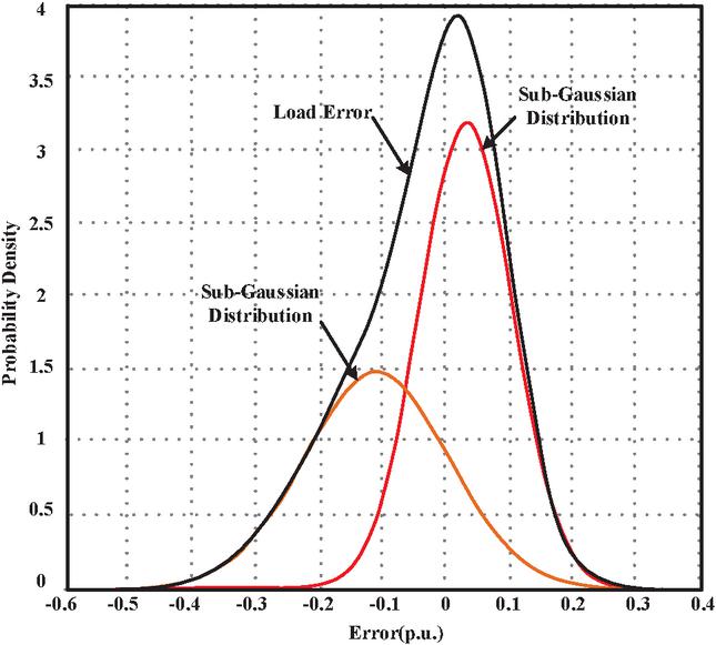
Figure 3 Probability distribution of load forecasting errors.
5 Case Studies
The analysis is conducted rely on an actual power grid’s real data in 2023, where the NE prediction deviation data refers to the actual prediction deviations that have occurred. Considering the load prediction error as a random variable, a Gaussian mixture model is adopted to fit the load prediction error. The number of Gaussian distributions is 2, with weights of (0.58, 0.42), expectations of (0.032, 0.109), and variances of (0.005, 0.013). The load forecast error is presented in Figure 3. This characteristic validates the necessity of the proposed three-layer framework of “data preprocessing-threshold adjustment-rolling dispatch”. Specifically, it enhances prediction accuracy through real-time updating of Pearson correlation coefficients to reduce scheduling instability caused by error accumulation.
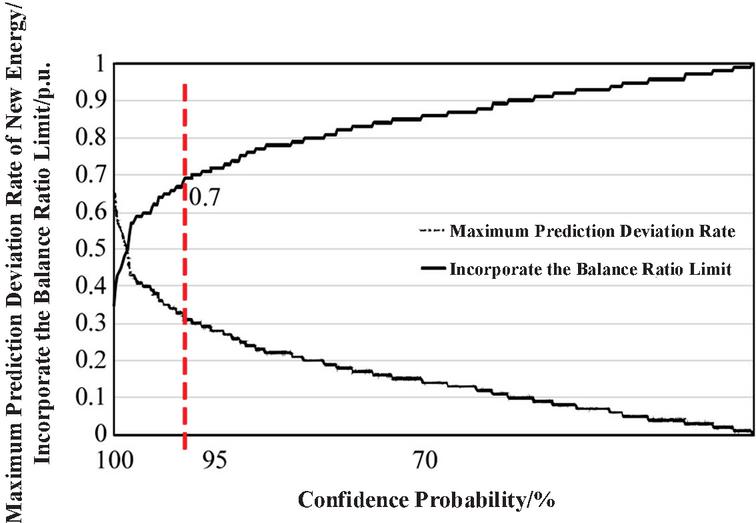
Figure 4 Relationship curves between the maximum prediction deviation rate of new energy in a certain actual power grid.
Based on the actual statistical data from 2021 to 2022, the function of the limit of the NE inclusion reserve ratio of the regional power grid concerning the confidence probability, namely F(f), as shown in Figure 4. In Figure 4, the thin dashed line depicts the relationship curve between the maximum prediction deviation rate of NE and the confidence probability. The thick solid line represents the limit of the new-energy inclusion reserve ratio corresponding to the confidence probability, denoted as F(f). Evidently, F(f) and f are negatively correlated. That is, as the confidence probability increases, the limit of the new-energy inclusion reserve ratio decreases. When the confidence probability is set at 95%, the limit of the new-energy inclusion reserve ratio is found to be 70%.
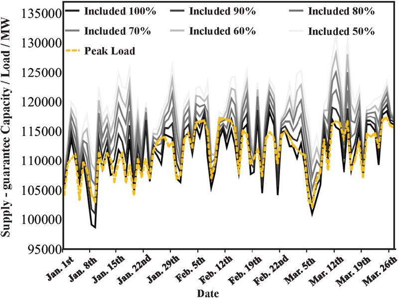
Figure 5 Daily maximum load curve of a regional power grid and daily maximum power supply.
Based on the first quarter of 2024 data from the same regional power grid, the power supply guarantee capabilities under different new-energy inclusion reserve ratios were calculated respectively. The comparison with the load curve is shown in Figure 5. It can be concluded that the higher the new-energy inclusion reserve ratio, the closer the power supply guarantee capacity curve is or lower than the peak-load curve. That is, the balance margin is smaller, and even a balance gap may occur. Conversely, the lower the new-energy inclusion reserve ratio, the more the power supply guarantee capacity curve tends to be or higher than the peak-load curve. That is, the balance margin is larger, and the possibility of a balance gap occurring is smaller.
After considering the reserve, the upper limit of the NE inclusion reserve ratio is affected by both the reserve and the predicted power output of NE at peak points, and it is no longer a constant under the same confidence probability. Based on the curve shown in Figure 6, when the confidence probability is selected as 95% and the corresponding regional power grid is equipped with reserves of 1 million kW, 2 million kW, 5 million kW, and 10 million kW respectively, the limit curves of the inclusion reserve ratio on different days in the first quarter.
Under the condition of the same reserve, the new-energy inclusion reserve ratio changes daily with the predicted output of renewable energy power. The larger the predicted output of renewable energy power, the smaller the inclusion reserve ratio. When the predicted new-energy power output is the same, the larger the reserve, the larger the limit of the new-energy inclusion reserve ratio. When the reserve is large enough, NE can be fully (100%) incorporated into the power balance. The results indicate a non-linear positive correlation between reserve capacity and new energy accommodation capability. This finding validates the design logic of the “reserve capacity as a flexible buffer layer” in the hierarchical regulation model, which can contain fluctuations from renewable sources within a safe range without significantly increasing grid investment.
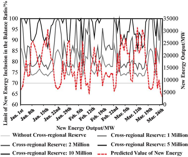
Figure 6 Limit curves of new energy inclusion reserve ratio under different reserves in the first quarter for a certain regional power grid.
6 Conclusion
The operation mechanism of the dispatchable units within the active distribution network has an essential impact on the dispatching solution. The research status of the dispatchable units within the active distribution network is analyzed from the “source” and “load” sides. Analyzing the working principle and development prospects of the dispatchable unit is important in preparing for the subsequent participation of distributed energy resources in the optimized dispatch of active distribution networks. This will be an important preparation for the study’s follow-up. A hierarchical prediction and control model for county power grids that considers factors such as new-energy prediction deviation, energy-storage regulation capability, and market price mechanism is developed. Ultimately, based on the cost-model study, the multi-objective elastic dispatch model of the county grid with cloud-side coordination and demand-side management strategies realizes the rolling dispatch in multiple time scales. This achieves the effect of reducing the fluctuation rate of new-energy utilization and further lowering the operation cost in the county. Future research could further integrate advanced information and communication technologies with power market mechanisms, deepen game theory modeling for multi-agent collaborative scheduling, and explore a county-level power grid resilient dispatching framework adapted to new power systems. This will provide more universal theoretical support and practical references for urban-rural energy transition under the “Double Carbon” goals.
Acknowledgment
Thanks to Professor Xiangyu Kong for the planning and implementation of this study, for proposing the research objectives and explaining how to carry out the research, and for finding and correcting the problems in time during the research process.
Funding Statement
This work is supported by the Science and Technology Project of State Grid Tianjin Electric Power Company (Ninghe-R&D 2023-01).
Author Contributions
Study conception and design: Chao Wang, Niu Yuan; data collection: Lei ZUO, Rui YU, Zhijun E; analysis and interpretation of results: Lei ZUO, Gaohua LIU; draft manuscript preparation: Chao Wang. All authors reviewed the results and approved the final version of the manuscript.
Availability of Data and Materials
Data available on request from the authors.
Conflicts of Interest
The authors declare that they have no conflicts of interest to report regarding the present study.
References
[1] E. Dokur, N. Erdogan, I. Sengor, U. Yuzgec and B. P. Hayes, “Near real-time machine learning framework in distribution networks with low-carbon technologies using smart meter data”, Applied Energy, vol. 384, pp. 125433–125433, 2025. https://doi.org/10.1016/j.apenergy.2025.125433.
[2] P. S. Georgilakis and N. D. Hatziargyriou, “A review of power distribution planning in the modern power systems era: Models, methods and future research”, Electric Power Systems Research, vol. 121, pp. 89–100, Apr 2015. https://doi.org/10.1016/j.epsr.2014.12.010.
[3] Y. Ma, X. Kong, L. Zhao, G. Liu and B. Gao, “A method for analyzing the irreparability of diverse electricity consumption data based on improved data generation technology”, Applied Energy, vol. 374, pp. 123994, Aug 2024. https://doi.org/10.1016/j.apenergy.2024.123994.
[4] J. Xiao, Z. Bao, C. Song, and G. Zu, “Selection Method of Power Flow Models Based on Capacity Boundary and Voltage Boundary”, Automation of Electric Power Systems, vol. 45, no. 20, pp. 76–83, 2021. https://doi.org/10.7500/AEPS20200803005.
[5] L. Wang, J. P. Zhou, W. J. Jiang, and Y. L. Xu, “Bi-level optimization configuration method for microgrids considering carbon trading and demand response”, Frontiers in Energy Research, vol. 11, Jan 2024. https://doi.org/10.3389/fenrg.2023.1334889.
[6] B. Gao, X. Kong, S Li, et al, “Enhancing anomaly detection accuracy and interpretability in low-quality and class imbalanced data: A comprehensive approach”, Applied Energy, vol. 353, Jan 2024, Art no. 122157. https://doi.org/10.1016/j.apenergy.2023.122157.
[7] H. Li and L. Lin, “Optimal Dispatch of CCHP Microgrid Considering Carbon Trading and Integrated Demand Response”, Distributed Generation and Alternative Energy Journal, vol. 35, no. 7, pp. 1681–1702, 2022. https://doi.org/10.13052/dgaej2156-3306.37516.
[8] J. Wu, G. De, Z. Tan, and Y. Li, “Study on bi-level multi-objective collaborative optimization model for integrated energy system considering source-load uncertainty”, Energy Science & Engineering, vol. 9, no. 8, pp. 1160–1179, Aug 2021. https://doi.org/10.1002/ese3.880.
[9] G. Cai, J. Zhou, Y. Wang, et al, “Multi-objective coordinative scheduling of system with wind power considering the regulating characteristics of energy-intensive load”, International Journal of Electrical Power & Energy Systems, vol. 151, Sep 2023, Art no. 109143. https://doi.org/10.1016/j.ijepes.2023.109143.
[10] B. Parrish, P. Heptonstall, R. Gross and B. K. Sovacool, “A systematic review of motivations, enablers and barriers for consumer engagement with residential demand response”, Energy Policy, vol. 138, p. 111221, Mar 2020. https://doi.org/10.1016/j.enpol.2019.111221.
[11] Z. Zhu, Z. Lin, L. Chen, et al, “Correlation knowledge extraction based on data mining for distribution network planning Global Energy Interconnection”, vol. 6, no. 4, pp. 485–492, Aug 2023. https://doi.org/10.1016/j.gloei.2023.08.008.
[12] M. Á. Lynch, S. Nolan, M. T. Devine and M. O’Malley, “The impacts of demand response participation in capacity markets”, Applied Energy, vol. 250, pp. 444–451, Sep 2019. https://doi.org/10.1016/j.apenergy.2019.05.063.
[13] Z. Rana H. A and M. Geev, “Active Distribution Network Operation: A Market-Based Approach”, IEEE Systems Journal, vol. 14, no. 1, pp. 1405–1416, Mar 2020. https://doi.org/10.1109/JSYST.2019.2927442.
[14] G. Muralikrishnan, K. Preetha, S. Selvakumaran, et al, “Optimal planning of photovoltaic, wind turbine and battery to mitigate flicker and power loss in distribution network”, Journal of Energy Storage, vol. 116, pp. 116116034, Mar 2025. https://doi.org/10.1016/j.est.2025.116034.
[15] Y. Zhang, A. Tsiligkaridis, I. Ch. Paschalidis, A. K. Coskun, “Data center and load aggregator coordination towards electricity demand response”, Sustainable Computing: Informatics and Systems, vol. 42, p. 100957, Apr 2024. https://doi.org/10.1016/j.suscom.2024.100957.
[16] C. Berk, S. Siddharth, R. Robin and H. Timothy M, “Quantifying the Impact of Solar Photovoltaic and Energy Storage Assets on the Performance of a Residential Energy Aggregator”, IEEE Transactions on Sustainable Energy, vol. 11, no. 1, pp. 405–414, Jan 2020. https://doi.org/10.1109/TSTE.2019.2892603.
[17] M. L. SwornaKokila, R. Venkatarathinam, J. P. Rose Bindu, M. A. Manivasagam, and K. H. Kishore, “Optimizing Energy Consumption in Smart Grids Using Demand Response Techniques”, Distributed Generation and Alternative Energy Journal, vol. 39, no. 1, pp. 111–136, 2024. https://doi.org/10.13052/dgaej2156-3306.3915.
[18] V. Rafi and P.K. Dhal, “An intelligent optimization technique for performance improvement in radial distribution network”, International Journal of Intelligent Unmanned Systems, vol. 13, no. 1, pp. 38–53, Feb 2025. https://doi.org/10.1108/IJIUS-04-2022-0052.
[19] B. Gao, X. Kong, G. Liu, et.al, “Monitoring high-carbon industry enterprise emission in carbon market: A multi-trusted approach using externally available big data”, Journal of Cleaner Production, vol. 466, p. 142729, Aug 2024. https://doi.org/10.1016/j.jclepro.2024.142729.
[20] G. Ma, S. Hu, N. Pang, and Q. Zhou, “Strategy Improved Pelican Algorithm Optimization ELM for Short-Term Electricity Load Forecasting”, Distributed Generation and Alternative Energy Journal, vol. 40, no. 1, pp. 85–108, 2025. https://doi.org/10.13052/dgaej2156-3306.4014.
Biographies

Chao Wang received the bachelor’s degree in Electrical Engineering and Its Automation from Huazhong University of Science and Technology in 2011. He is currently working at the Dispatch and Control Center of State Grid Tianjin Ninghe Electric Power Supply Company. His research areas include power system planning and operation, power system protection and control, etc.

Yuan Niu graduated from the School of Electronic Information Engineering of University of Electronic Science and Technology of China in 2005. He is currently working at the Dispatch and Control Center of State Grid Tianjin Ninghe Electric Power Supply Company. His research areas include power system planning and operation, practical technologies for the safe and economic operation of smart grids, etc.

Lei Zuo received the bachelor’s degree in Electrical Engineering from Chongqing University in 2016 and the master’s degree in Electrical Engineering and Automation from Tianjin University in 2019. He is currently working at the Dispatch and Control Center of State Grid Tianjin Electric Power Company. His research areas include power system planning and operation, as well as grid simulation and analytical computation.

Rui Yu graduated from Tianjin University in 2024. He is currently studying for a master’s degree at Tianjin University. The main research interests include new energy scenario generation and distribution network dispatching.

Gaohua Liu received the B.Eng. degree in communication engineering from Qindao Science and Technology University, Shandong, China, in 2010, and the M.E. degree in electromagnetic field and microwave technology from Tianjin University, Tianjin, China, in 2013, where she is currently pursuing the Ph.D. degree in information and communication engineering. Since 2013, she has been with the School of Electronics and Information Engineering, Tianjin University. Her main research interests include deep learning-based behavior analysis and interaction system development.

Zhijun E received the bachelor’s degree in Electrical Engineering and Automation from Tianjin University in 2000 and the doctor’s degree in Electrical Engineering and Automation from Tianjin University in 2008 He is currently working at the Dispatch and Control Center of State Grid Tianjin Electric Power Company. His research areas include power system planning and operation, as well as grid simulation and analytical computation.
Distributed Generation & Alternative Energy Journal, Vol. 40_4, 655–680.
doi: 10.13052/dgaej2156-3306.4042
© 2025 River Publishers