Multi-Terminal Transmission Line Fault Localization Based on 1dCNN-Transformer
Shan Rui1, He Jiaxi2, Pan Weifeng1, Ma Jinlong1, Yang Jiahui1 and Guo Ningming2
1State Grid Ningxia Ultrahigh Voltage Company, Yinchuan 750011, China
2C-EPRI Electric Power Engineering Co., Ltd., Beijing 102200, China
E-mail: 17801790602@163.com
*Corresponding Author
Received 26 May 2025; Accepted 21 September 2025
Abstract
Aiming at the problem of difficult extraction of fault traveling-wave front of transmission line faults, this paper proposes a fault traveling-wave front extraction method based on the combination of Variational Mode Decomposition (VMD) and Teager Energy Operator (TEO). First, the fault current traveling wave signal is decoupled by the Karenbauer transform to obtain the -mode component, and then the VMD decomposition is implemented on this component, and the decomposed IMF3 component is selected, and the TEO energy operator is applied to determine the arrival time of the head. Aiming at the problem of missing detection point data in multi-terminal transmission line fault localization, a method combining 1dCNN-Transformer neural network and double-ended traveling wave ranging formula is proposed. The fault feature information is input into the 1dCNN-Transformer to identify the fault section, and then the distance of the fault point is calculated according to the arrival time of the wave head and using the double-ended traveling wave ranging formula. A 750 kV multi-terminal transmission line fault simulation model is constructed using the PSCAD/EMTDC platform, and the simulation results prove that the proposed method is still able to identify fault zones in the case of missing data at detection points, and the error of the fault ranging results is within 100 m.
Keywords: Transmission lines, variational mode decomposition, Teager energy operator, 1dCNN-transformer neural network.
1 Introduction
In the modern power system, 750 kV transmission lines undertake the important task of large-scale power transmission, and their safe and stable operation is crucial for guaranteeing power supply [1, 2]. However, because the transmission line is located in a complex environment, affected by a variety of factors, faults occur from time to time, and the problem of missing data at the detection point has a huge impact on fault localization. Accurately and quickly locating the fault location is extremely important for timely repair of faults and reduction of outage time and economic losses.
Research on 750 kV multi-terminal transmission line fault localization has progressed along three main directions: traveling wave-based approaches [3–5], impedance-based methods [6, 7], and artificial intelligence-based techniques [8–10]. The impedance method, while simple in principle, is heavily affected by network topology, line parameters, and fault position, which restricts its reliability and range of application. Traveling wave approaches, such as the fault discrimination matrix [11], improved double-ended ranging for high-voltage lines [12], and NGO-optimized VMD decomposition [13], can achieve accurate fault distance estimation and improved robustness in noisy environments, but they remain less effective when dealing with missing detection data or the complex structure of multi-terminal systems. Artificial intelligence-based methods have attracted increasing attention, with examples including parallel CNN frameworks that jointly identify fault types and sections in multi-terminal DC networks [14], neural network mappings capable of adapting to hybrid overhead–cable configurations [15], and lightweight LSSVM models for DC single-pole grounding faults with strong real-time performance [16]. These methods demonstrate high efficiency in feature learning and section recognition, but they still face challenges such as insufficient discussion of traveling-wave physical mechanisms, limited transferability from DC to AC multi-terminal systems, weaker generalization to large-scale networks with changing topologies, and unverified robustness under missing or incomplete measurements. Although different neural network-based approaches [17–19] have shown significant improvements in classification accuracy, they are typically more effective for fault section identification than for precise fault distance prediction. In summary, traveling wave-based methods excel at accurate distance calculation but struggle with multi-terminal adaptability and incomplete data, while artificial intelligence approaches provide strong section identification capabilities but often suffer from relatively large ranging errors and unresolved engineering constraints.
To address the above problems, this paper proposes a multi-terminal transmission line fault localization method combining 1dCNN-Transformer neural network and double-ended traveling wave ranging. First of all, the fault current data needs to be preprocessed, and the -mode component obtained from the decoupling transform of the fault current data is decomposed by VMD; then the IMF3 component obtained after the decomposition is input into the 1dCNN-Transformer neural network as a fault feature to identify the fault location; after that, the fault traveling-wave front is labeled by using the TEO energy operator to obtain the fault initial traveling wave arrival time at the detection point, and then the double-ended traveling wave ranging method is used to locate the fault. Subsequently, the TEO operator marks the initial arrival of the faulty traveling wave, and the fault distance is calculated using the double-ended ranging method. Finally, the proposed method is validated through PSCAD/EMTDC simulations.
2 Data Preprocessing
The current traveling wave will be coupled between the three phases during the propagation process, which requires decoupling of the phase currents. In this paper, the Karenbauer transform is used to decouple the phase currents. Since there are many cluttered signals in the fault current data obtained at the detection point, and it is difficult to extract the fault traveling-wave front directly, this paper chooses the VMD decomposition method to decompose the components obtained after decoupling, remove the cluttered signals, and obtain the components with rich fault characteristic information.
2.1 Karenbauer Transformation
The Karenbauer transform is a method capable of decoupling three-phase currents, which converts three-phase currents into modal components using a specific matrix of the form:
| (1) |
Where , , are the original three-phase currents, and , , are the transformed mode components. is the ground mode component after decoupling, and and are the line mode components after decoupling. The current traveling wave is transformed by the Karenbauer transform to obtain the ground mode component (mode 0) and the line mode components (mode and ), in which the ground mode component attenuates more seriously in the propagation process, so the mode component is used for the analysis in this paper.
2.2 Variational Mode Decomposition
VMD is a state-of-the-art signal processing method that overcomes the modal aliasing and end-point effects of traditional methods by adaptively decomposing complex signals into multiple Intrinsic Mode Functions (IMFs) with sparsity and center frequencies [20]. The problem of modal aliasing and endpoint effect of traditional methods is overcome. It transforms the signal decomposition into a variational optimization problem, where the goal is to find a set of modal functions and their corresponding center frequencies such that the sum of the bandwidths of all the modes is minimized, while guaranteeing that the sum of the modes is equal to the original signal. The mathematical model is:
| (2) | |
| (3) |
where is the kth modal component, is the corresponding center frequency, and is the original signal.
In this paper, the -mode component is subjected to VMD decomposition with a penalty factor of 2000 and a number of decomposition layers of 4. Taking the data obtained from the fault point located in faulty section 1 and 35 km away from the detection point I1 35 km, with a transition resistance of 300 , and the data obtained from the detection point I1 as an example, its VMD decomposition obtains the various IMF components as shown in Figure 1. From Figure 1, it can be seen that the IMF3 component has obvious sudden variation features and rich fault characteristic information, which is easy to extract the fault traveling-wave front.
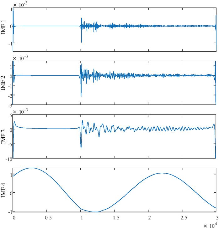
Figure 1 VMD decomposition diagram.
3 Fault Zone Localization
3.1 1dCNN-Transformer Neural Network
In the field of neural networks, Convolutional Neural Networks (CNNs) are particularly effective for localized feature extraction through the use of convolutional kernels, offering significant advantages over traditional machine learning methods and other deep learning architectures. A one-dimensional Convolutional Neural Network (1dCNN) is a specialized variant designed for sequential data, where the core operation is convolution along a single dimension [21, 22]. A typical CNN architecture consists of an input layer, one or more convolutional and pooling layers, followed by fully connected and output layers, with convolutional and pooling layers repeated as required by the network design. Unlike other classical neural networks, CNNs adopt a parameter-sharing mechanism, in which all neurons in a convolutional layer share the same weight parameters. This approach greatly reduces computational complexity while enabling each neuron to focus on a single feature, thereby preserving the integrity of the extracted data representations.
Transformer has now gradually replaced RNN models such as LSTM as the architecture of choice in the field of temporal data processing. A Transformer unit consists of several parts, including a position coding layer, a multi-head self-attention layer, a feed-forward network layer, and a layer normalization module. The structure of the Transformer unit is shown in Figure 2, in which the attention mechanism Transformer’s core [23, 24].
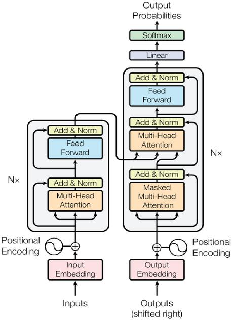
Figure 2 Transformer unit structure.
Attention Mechanism is a data processing method in machine learning, which is a technique that mimics the way human attention is focused [25]. Attention Mechanism makes the model more able to focus on more important parts while ignoring irrelevant content. For traditional time-series networks, the parts of the input to the network layer usually have the same weight. Attention mechanisms, on the other hand, allow different weights to be attached to different parts, thereby capturing more critical features. A typical attention mechanism is given in the following equation:
| (4) |
Where: Q represents the query vector (Query), that is, the input query vector; K represents the key vector (Key), that is, the potential feature representation of the input value; V represents the value vector (Value), that is, the output feature representation of the input information; represents the dimension of the key vector.
The attention mechanism can be divided into two parts: (1) calculating the similarity or correlation between Q and K to get the weight coefficients against V; (2) multiplying the weight coefficients with V to get the final attention score. Unlike RNN network architectures such as LSTM, Transformer is implemented using the attention mechanism rather than a different gate structure. The Transformer architecture consists of encoders and decoders, each of which consists of layers containing self-attention and feed-forward neural networks with a large number of parameters themselves. In general, the larger the model’s number of parameters, the higher the model’s relative fit to the data. Since the attention mechanism operates on the entire feature vector, retaining information over the entire feature dimension, the attention mechanism is particularly suitable for tasks with long sequences and high-dimensional feature inputs.
The 1dCNN-Transformer neural network used in this paper is a 1dCNN that first extracts the local features of the sequence, then inputs the feature vector into the Transformer module to further extract the entire sample in the global features, and finally the fully-connected layer outputs the results of fault section identification.
3.2 1dCNN-Transformer Based Fault Section Identification Method
The classification network in this paper consists of three sub-modules which are Convolutional Module, Transformer Module and Classification Module. In the convolution module, a Batch Norm layer is used along with a two-layer convolutional network for extracting local features of the sequence. After the convolution module, a Dropout layer is used to accelerate the training and prevent overfitting. The number of layers in the Transformer layer is 2, where each Transformer unit has four attention heads, followed by still the same Dropout layer as in the previous section. Finally, there is the classification module, which consists of two fully connected layers that output the probability of the corresponding category. The parameters of each module are shown in the following table.
Table 1 Classification network parameters
| System Parameter | Parameter Value |
| Convolutional Module Layer 1 | 64 |
| Convolutional Module Layer 2 | 64 |
| Dropout Layer | 20% |
| Transformer module layer 1 | 64 |
| Transformer module layer 2 | 64 |
| Dropout Layer Discard Rate | 20% |
| Classification module layer 1 | 64 |
| Classification module layer 2 | 128 |
| Input layer | 8 |
| 0utput layer | 5 |
| Learning rate | 0.001 |
| Maximum training rounds | 200 |
| Batch Size | 8 |
In order to enhance the saliency of fault features, this paper introduces flag bits for the IMF3 component of each detection point. The flag bits are defined as all data points before the mutation of the IMF3 component are labeled as 0, while all data points after the mutation are labeled as 1. Subsequently, the IMF3 component of each detection point and its corresponding flag bits are jointly inputted into the 1dCNN-Transformer neural network as a fault feature with the corresponding fault section as the output target of the model.
4 VMD-TEO Based Double-Ended Traveling Wave Localization
4.1 Double-Ended Traveling Wave Positioning Principle
When a fault occurs on a line, the resulting transient voltage and current waves propagate along the line to both ends. The propagation speed of these traveling waves is close to the speed of light, so the time difference between reaching the two ends can be used to calculate the fault location. The principle of double-ended traveling wave localization is shown in Figure 3.
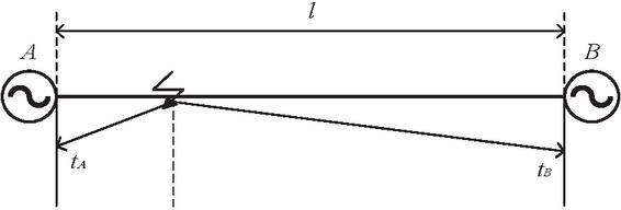
Figure 3 Schematic diagram of double-ended traveling wave localization.
The formula for calculating the distance from the fault point to the detection point using the time difference is shown below:
| (5) |
where and are the time for the initial traveling wave of the fault to reach the detection points at both ends, l is the length of the transmission line, , L and C are the inductance and capacitance per unit length of the line, respectively.
4.2 VMD-TEO Fault Traveling-Wave Front Detection
The use of double-ended traveling wave localization method is based on the premise that the initial traveling wave of the fault needs to arrive at both ends of the monitoring point, which requires accurate capture of the fault traveling-wave front, usually using the energy operator to amplify the sudden variation features of the signal to achieve the purpose of capturing the fault traveling-wave front. In this paper, the classical TEO is used to capture the fault traveling-wave front.
TEO is a nonlinear signal processing tool that is mainly used to analyze the instantaneous energy characteristics of non-smooth signals. The core idea is to estimate the instantaneous energy of a signal through the local dynamic characteristics of the signal. The mathematical definition of TEO is shown below:
| (6) | ||
| (7) |
where Equations (6) and (7) are mathematically defined for discrete signals x[n] and continuous signals x(t).
Since the IMF3 component obtained after VMD decomposition has rich sudden variation features, this paper adopts the TEO to label the fault traveling-wave fronter of the IMF3 component of the current at each detection point. Taking the fault point located in fault zone 1 and 35 km from the detection point I1, the transition resistance is 300, the data of each detection point as an example, the fault initial fault traveling-wave fronter labeling diagram is shown in Figure 4. As can be seen in Figure 4, the faulty fault traveling-wave front can be clearly marked using VMD-TEO.
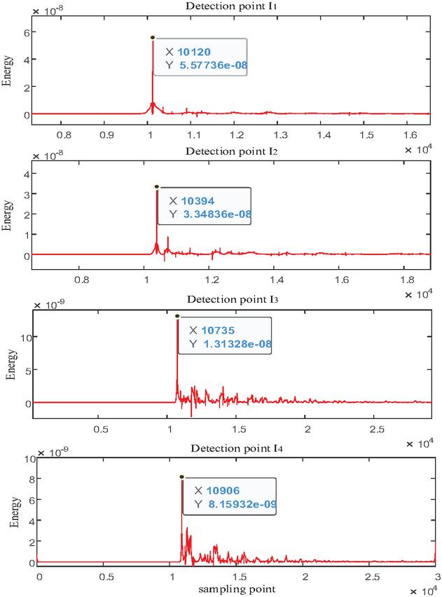
Figure 4 Faulty initial fault traveling-wave front marking map.
From the above, it can be seen that in this paper, we first use the method of combining VMD and TEO energy operator to get the time of the initial traveling wave of the fault arriving at each detection point, and then calculate the distance of the fault point from the detection point according to the method of double-ended traveling wave localization.
5 Multi-Terminal Transmission Line Fault Localization Process
By comprehensively analyzing the previous two sections, it can be seen that the 1dCNN-Transformer-based fault segment identification technique and the double-ended traveling wave ranging method have significant complementary advantages. Specifically, the 1dCNN-Transformer neural network can accurately determine the line segment where the fault occurs and is not affected by the lack of data at the detection point, while the double-ended traveling wave localization technique can accurately calculate the distance between the fault point and the measurement end. By organically combining these two methods, a complete set of fault localization solutions can be constructed, thus realizing the high-precision determination of the fault location of multi-terminal transmission lines. Its specific realization process is:
(1) After the current data are collected at the detection point, the current signal collected at the detection point is modally decoupled using the Karenbauer transform, which effectively eliminates the interphase coupling effect of the line and obtains the pure -mode component signal.
(2) Adaptive decomposition of the -mode component by the VMD algorithm is performed to obtain the IMF3 component containing the fault mutation features. Subsequently, the TEO energy operator of the IMF3 component is calculated to accurately capture the characteristics of the moment when the initial fault traveling-wave front of the fault arrives at the detection point.
(3) The IMF3 components with sudden variation features and their flag bits are input as fault features into the 1dCNN-Transformer to determine the zone where the fault point is located.
(4) On the basis of determining the fault section, combined with the principle of double-ended traveling wave ranging, using the wave head arrival time difference and traveling wave propagation speed, the precise distance between the fault point and the detection end is finally calculated, to complete the precise fault location of multi-terminal complex transmission network.
The positioning flowchart is shown below:
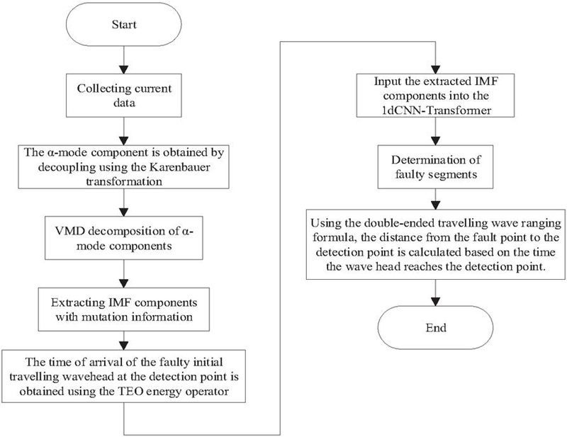
Figure 5 Fault localization flowchart.
6 Simulation Verification
6.1 Simulation Model
As shown in Figure 6, a four-terminal overhead transmission line model was built for fault simulation using the electromagnetic transient program PSCAD/EMTDC. In this system, the node serves as the demarcation point: the line between detection points I1 and I4 is divided into three zones (0, 1, and 2), the line between detection points I2 and node T1 is divided into four zones, and the line between detection point I3 and node T2 is divided into five zones. Sections 0–2 are each 100 km in length, while sections 3 and 4 are each 50 km. The detailed line parameters are given in Table 2. A fault is initiated at 0.3 s and lasts for 0.1 s. The sampling frequency is set to 1 MHz, and the sampling window covers 0.29–0.32 s. The parameters of the power-source model are given in Table 3.
Since the accuracy of traveling-wave detection is a critical factor for precise fault location – the waves propagate from the fault point at nearly the speed of light, requiring highly accurate detection of their arrival times at both terminals – the detectors operate at 1 MHz, corresponding to a 1 s sampling interval, to ensure reliable wave-head capture. To balance engineering feasibility with localization accuracy, an event-triggered short-window high-sampling scheme is adopted: during normal operation, the device maintains 4 kHz sampling of power-frequency quantities to support conventional protection functions; once a fault occurs, a transient channel is activated at 1 MHz for a 20–30 ms window to perform traveling-wave-based localization.
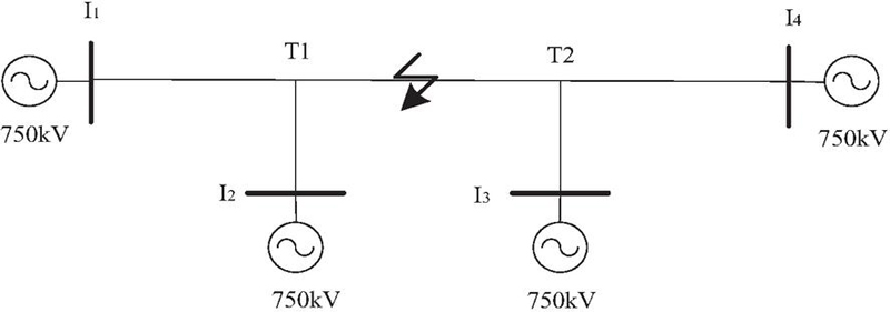
Figure 6 Simulation diagram.
Table 2 Line parameters
| Phase Sequence | ||
| Line Parameters | Positive Sequence | Zero Sequence |
| Resistive/(km-1) | 0.03468 | 0.3 |
| Inductors/(mHkm-1) | 1.3477 | 3.637 |
| Capacitors/(Fkm-1) | 0.00867 | 0.00616 |
Table 3 The parameters of the power-source model
| Power-source | Z1 | Z0 |
| I1 | 1.052+j23.175 | 0.600+j19.091 |
| I2 | 1.050+j21.925 | 0.300+j17.436 |
| I3 | 1.046+j18.765 | 0.390+j14.861 |
| I4 | 1.049+j22.106 | 0.590+j19.372 |
6.2 Fault Section Verification
Faults are set up at specific locations in five different zones, simulation operations are carried out, and then the current data of each detection point are obtained, which together form the data sample. The specific content of the data sample is shown in Table 4.
Table 4 Sample data
| Sample Name | Numerical Value |
| Fault type | Phases A, B, and C are shorted to ground. |
| Transition resistance () | 0.01, 100, 200, 300, 400 |
| Total line length (km) | 400 |
| Failure interval (km) | 5 |
| Sample size | 1200 |
The data samples are divided into a training set and a test set with a ratio of 8:2. where the training set accounts for 80% of the entire data samples and the test set accounts for 20%. The training set and test set are input into the 1dCNN-Transformer model together, and the results of fault section recognition are shown in Figure 7. As can be seen from Figure 7, the accuracy of fault section identification reaches 100%, indicating that the 1dCNN-Transformer neural network used in this paper is able to perfectly determine the zone where the fault is located.
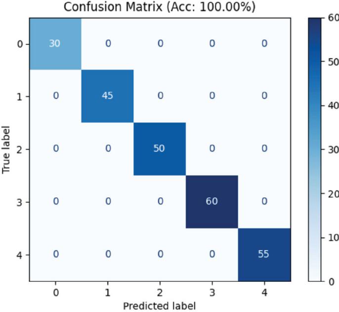
Figure 7 Fault section prediction results.
In order to verify that the method will not be affected by the missing data of the detection points, all the data of a certain detection point in each group of data are deleted and input into the model again, and the results are shown in Figure 8. From Figure 8, we know that when the data of a certain detection point is missing, the recognition accuracy of the fault section also reaches 100%, which indicates that the method can solve the problem of missing data of the detection point.
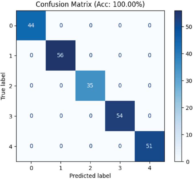
Figure 8 Fault section prediction results when detection point data is missing.
6.3 Comparative Experiment with Other Models
To further verify the superiority of the proposed method, comparative experiments were conducted with classical machine learning and neural network models, including BP neural network and SVM. The same data set and experimental environment were used, and the evaluation indicators were classification accuracy, model training runtime, and diagnosis time for a single sample. The results are shown in Table 5.
Table 5 Comparative performance of different models for fault section identification
| Model | Accuracy | Model Training Runtime(s) | Diagnosis Time(s) |
| CNN-Transformer | 100% | 385.41 | 0.014 |
| BP | 93.75% | 337.83 | 0.036 |
| SVM | 96.25% | 426.37 | 0.021 |
As can be seen from Table 5, although the training runtime of the CNN-Transformer model is slightly longer than BP, it achieves the highest classification accuracy and the shortest diagnosis time. Compared with BP and SVM, the proposed method demonstrates stronger generalization ability and faster real-time performance in fault segment identification, which further confirms its engineering applicability.
6.4 Determination of Fault Distance
In order to accurately locate the fault location in a multi-terminal transmission line, after determining the section where the fault is located, it is necessary to further clarify the distance between the fault point and the detection point. In this paper, the double-ended traveling wave ranging method is applied to carry out the calculation of this distance. Specific steps are: first, through the combination of VMD and TEO energy operator, the initial fault traveling-wave front of the fault is labeled, so as to obtain the initial traveling wave of the fault arrives at each detection point time. Then, based on the relevant parameters of the transmission line, the wave speed of the traveling wave is determined to be 292545 km/s. Finally, based on the arrival time of the traveling wave at each detection point and the known wave speed, the specific distance of the fault point from the detection point is calculated.
Table 6 Fault distance calculation results
| Parameters | |||
| Zones | Practical Distance (km) | Calculated Distance (km) | Error (km) |
| 1 | 35 | 34.9213 | 0.0787 |
| 65 | 65.0157 | 0.0157 | |
| 2 | 135 | 135.0802 | 0.0802 |
| 165 | 164.9198 | 0.0802 | |
| 3 | 235 | 234.9843 | 0.0157 |
| 265 | 264.9702 | 0.0298 | |
| 4 | 25 | 24.9748 | 0.0252 |
| 35 | 34.9213 | 0.0787 | |
| 5 | 25 | 24.9747 | 0.0253 |
| 35 | 34.9213 | 0.0787 | |
In this paper, the data of the following cases are selected for the validation of the fault distance: zone 1 is 35 km and 65 km away from the detection point I1, zone 2 is 135 km and 165 km away from the detection point I1, zone 3 is 235 km and 265 km away from the detection point I1, zone 4 is 25 km and 35 km away from the detection point I2, and zone 5 is 25 km and 35 km from detection point I3. Through the validation of these data, the final results are shown in Table 6.
From the data in the table, the maximum error of the distance is 80.2 m, which is within 100 m, indicating that the method is highly accurate and has a certain degree of effectiveness and feasibility.
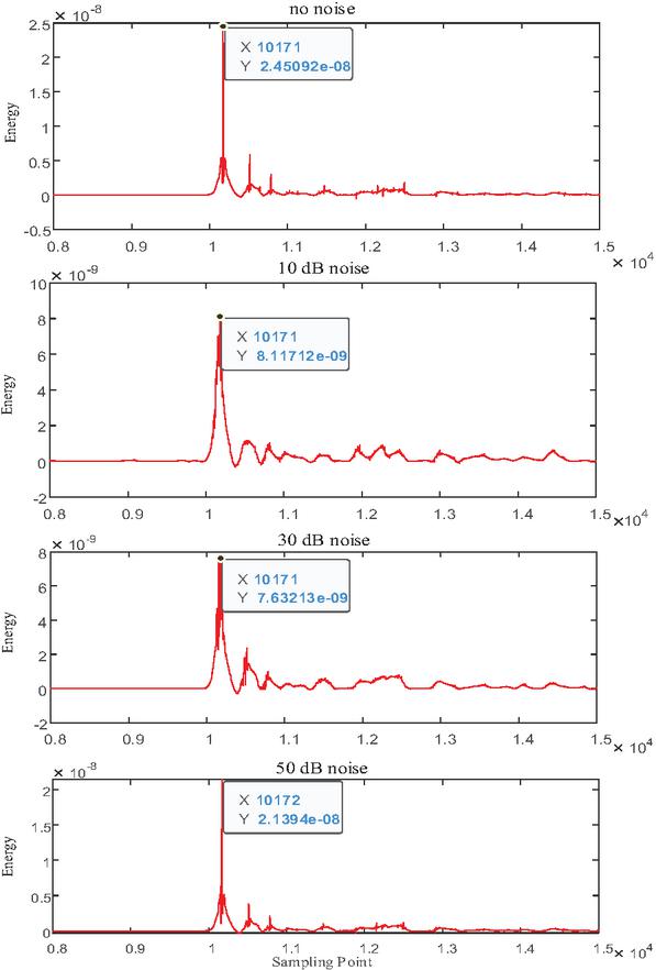
Figure 9 Influence of different noise levels on fault traveling-wave front detection.
6.5 Influence of Noise
To further evaluate the robustness of the proposed fault location method under realistic operating conditions, the influence of noise was investigated. In practice, fault traveling-wave signals are inevitably contaminated by noise introduced by electromagnetic interference, switching operations, and measurement devices. In this study, Gaussian white noise of different levels was added to the original fault current signals, with signal-to-noise ratios (SNR) of 10 dB, 30 dB, and 50 dB, respectively. The results are shown in Figure 9.
As illustrated in Figure 9, even with noise contamination, the abrupt change corresponding to the fault traveling-wave front can still be effectively captured by the VMD–TEO operator. Specifically, when the SNR is as low as 10 dB, although the overall waveform exhibits significant fluctuations, the fault wavefront remains clearly distinguishable at approximately the same sampling point (around 10171–10172). With higher SNR levels (30 dB and 50 dB), the noise impact becomes progressively weaker, and the detected wavefront coincides almost perfectly with the noise-free case.
These results demonstrate that the proposed VMD–TEO-based wavefront detection method exhibits strong noise suppression capability and ensures accurate fault localization under different noise conditions.
7 Conclusion
(1) In view of the fact that the fault discrimination matrix may be affected by the missing detection points, this paper proposes a fault segment identification method based on 1dCNN-Transformer neural network. The principle of this method is concise and clear, the operation process is simple and easy, and the recognition accuracy is high, which can effectively avoid the problems caused by the missing detection points, and has good feasibility.
(2) In this paper, a method combining the VMD with the TEO energy operator for labeling the initial fault traveling-wave front is proposed, and it is coupled with the double-ended traveling wave ranging formula to accurately calculate the distance between the fault point and the detection point. The simulation results show that the error of the distance calculated by this method can be controlled within 100 m with high accuracy.
(3) The proposed multi-terminal transmission line fault location method remains capable of reliably detecting the fault traveling-wave front under different noise levels and achieves superior accuracy, robustness, and generalization compared with conventional methods, ensuring reliable location results and highlighting its engineering value and potential for application in complex power systems.
Acknowledgements
State Grid Ningxia Electric Power Co., Ltd.: Development and Application of Grid Fault Location System Based on Autonomous and Controllable Platform and Multi-source Data (5229CG24000K).
References
[1] Han Xiancai, Sun Xin, Chen Haibo, et al. Overview of the development of China’s extra-high voltage AC transmission engineering technology[J]. Chinese Journal of Electrical Engineering, 2020, 40(14):4371–4386+4719.
[2] Mengzhao D, Yu L, Dian L, et al. A novel noniterative single-ended fault location method with distributed parameter model for AC transmission lines[J]. International Journal of Electrical Power and Energy Systems, 2023, 153.
[3] Wang Si Hua, Wang LingBai. A double-ended flexible DC transmission fault ranging scheme based on SAO-VMD-S[J]. Power System Protection and Control, 2025, 53(01):1–12.
[4] Wei C, Dong W, Donghai C, et al. Novel travelling wave fault location principle based on frequency modification algorithm[J]. International Journal of Electrical Power and Energy Systems, 2022, 141.
[5] Li Chengxin, Liu Guowei, Yu Cong, et al. Fault localization method for high-voltage transmission lines based on traveling waves[J]. Journal of Electric Power Science and Technology, 2023, 38(02):179–185.
[6] Xu Mingming, Wang Junjie, Dong Xuan, et al. Offline localization method for overhead line faults based on satellite timing[J]. Global Energy Internet, 2024, 7(05):530–540.
[7] Zhang Haiyue, Wang Shouming, Liu Ji, et al. Cable fault diagnosis and localization based on digital reconstruction of PT-PFM excitation impedance spectrum[J]. Chinese Journal of Electrical Engineering, 2024, 44(02):805–817.
[8] Yu Li, Jiao Zhibin, Wang Xiaopeng, et al. Precise fault localization method and key technology of medium voltage distribution network based on PMU[J]. Power System Automation, 2020, 44(18):30–38.
[9] Chen Xiaolong, Sun Lirong, Li Yongli, et al. Asynchronous fault ranging algorithm for double-ended transmission lines based on artificial neural network and network migration[J]. Grid Technology, 2023, 47(12):5169–5181.
[10] Nsed V O, Sajjad H, A.A. K. G. The use of artificial neural network for low latency of fault detection and localisation in transmission line[J]. Heliyon, 2023, 9(2): e13376–e13376.
[11] Li Lianbing, Sun Tengda, Zeng Siming, et al. Distribution network fault localization method based on multi-terminal traveling wave time difference[J]. Power System Protection and Control, 2022, 50(03):140–147.
[12] Yu Zexuan, Pazlai Mahmuti. Fault localization of high-voltage AC transmission line based on improved double-ended method[J]. Optoelectronics-Laser, 2021, 32(10):1099–1104.
[13] Yu K, Zhu X, Cao W. Study on Traveling Wave Fault Localization of Transmission Line Based on NGO-VMD Algorithm[J]. Energies, 2024, 17(9).
[14] Wang H, Yang D, Zhou B, et al. Fault diagnosis of multi-terminal HVDC transmission lines based on parallel convolutional neural networks. Automation of Electric Power Systems, 2020, 44(12):84–92.
[15] T. Li, Y. Han, Z. Jiao and Y. Mu, Fault Location of Hybrid Three-terminal HVDC Transmission Line Based on Neural Network, 2019 IEEE 3rd International Electrical and Energy Conference (CIEEC), Beijing, China, 2019, 1717–1722.
[16] K. Wei, S. Lan and Z. Li, Single-Pole Ground Fault Location Method for Multi-terminal Flexible DC Transmission Lines Based on LSSVM, 2022 12th International Conference on Power and Energy Systems (ICPES), Guangzhou, China, 2022, 214–218.
[17] He Xiaolong, Gao Hongjun, Huang Yuan, et al. A fault segment localization method for distribution networks based on one-dimensional convolutional and graph neural networks[J]. Power System Protection and Control, 2024, 52(17):27–39.
[18] Xinghua W, Peng Z, Xiangang P, et al. Fault location of transmission line based on CNN-LSTM double-ended combined model[J]. Energy Reports, 2022, 8(S5):781–791.
[19] Qi Sheng-long, Lu Xiang, Liu Haitao, et al. Application of BP neural network in distribution network fault diagnosis based on genetic algorithm optimization[J]. Journal of Electric Power Science and Technology, 2023, 38(03):182–187+196.
[20] Xu, Z., Xiang, K., Wang, B., and Li, X. (2024). Study on PV Power Prediction Based on VMD-IGWO-LSTM. Distributed Generation & Alternative Energy Journal, 39(03), 507–530.
[21] Zhang Chao, Qin Min-Min, Zhang Shao-Fei. Rolling bearing fault diagnosis based on 1D CNN-XGBoost[J]. Machine Tools and Hydraulics, 2022, 50(16):169–173.
[22] Singirikonda, S., and Obulesu, Y. P. (2023). Lithium-Ion Battery State of Charge Estimation Using Deep Neural Network. Distributed Generation & Alternative Energy Journal, 38(03), 761–788.
[23] Chen, H., Meng, L., Xi, Y., Xin, M., Yu, S., Chen, G., and Chen, Y. (2023). GRU Based Time Series Forecast of Oil Temperature in Power Transformer. Distributed Generation & Alternative Energy Journal, 38(02), 393–412.
[24] Zhang Jianliang, Han Tao, Ji Ruisong. Fault diagnosis design of medium voltage DC all-electric propulsion system for ships based on CNN-BiLSTM-Transformer[J]. Experimental Technology and Management, 2025, 42(01):11–18.
[25] Chen, Z., Yang, L., Tian, J., Chen, Z., Xu, X., and Zhao, E. (2023). Real-time Monitoring Technology of Voltage Sag Disturbance in Distribution Network Based on TCN-Attention Neural Network and Flink Flow Computing. Distributed Generation & Alternative Energy Journal, 38(05), 1637–1658.
Biographies

Shan Rui, born in May 1972, male, a native of Xi’an, Shaanxi Province, Han nationality, graduated from Hefei University of Technology in 1995 with a bachelor’s degree, majoring in electronic engineering. He is now a senior engineer of State Grid Ningxia UHV Company. His main research direction is relay protection and automatic device, and since February 2012, he has been engaged in relay protection and dispatching automation management in State Grid Ningxia UHV Company. He has published 10 academic papers, participated in 7 research projects and 4 other academic research achievements.

He Jiaxi, born in June 1998, female, Han nationality, Daqing, Heilongjiang Province, graduated from Harbin Institute of Technology in 2020, majoring in electrical engineering and automation, and obtained a bachelor’s degree in engineering. She is now working as an electrical engineer in CLP Power Engineering Co., Ltd. and is mainly engaged in the technical research and engineering application of power system related fields.
Pan Weifeng, born in May 1982, male, Han nationality, Xi’an, Shaanxi. He undertakes research work in electrical engineering and automation at State Grid Ningxia Ultrahigh Voltage Company.
Ma Jinlong, born in April 1993, male, Hui nationality, is from Wuzhong, Ningxia. He undertakes research work in electrical engineering and automation at State Grid Ningxia Ultrahigh Voltage Company.
Yang Jiahui, born in January 1993, male, Hui nationality, is from Shizuishan, Ningxia. He is working in State Grid Ningxia Ultrahigh Voltage Company in the field of secondary operation and inspection technology of substation.
Guo Ningming, born in May 1980, male, Han nationality, Fuzhou, Fujian Province. He undertakes research work in high voltage and insulation technology at C-EPRI Electric Power Engineering Co.
Distributed Generation & Alternative Energy Journal, Vol. 41_1, 145–166
doi: 10.13052/dgaej2156-3306.4117
© 2026 River Publishers