Design of an Electrical Fault Diagnosis Method Incorporating Compressed Sensing and Wavelet-SVM
Shukai Liu
School of Intelligent Manufacturing, Changzhou Vocational Institute of Engineering, Changzhou, 213164, China
E-mail: Shukai_Liu@outlook.com
Received 12 June 2025; Accepted 09 July 2025
Abstract
The building’s electrical system is crucial, and when a defect arises, it not only necessitates power outages and maintenance, which results in financial losses, but also interferes with people’s regular output and way of life. To a certain extent, the regular operation of building electrical facilities and equipment depends heavily on the development of problem diagnosis technology in the field of building electrical. Based on this, the study suggests a fault diagnosis model for support vector machines and K closest neighbors that incorporates compressive sensing and wavelet transform. The approach improves the K-nearest neighbor algorithm while using a support vector machine as the training framework. This increases the algorithm’s operational efficiency and diagnostic accuracy while also enhancing the support vector machine’s ability to handle huge sample sizes of data. The model uses wavelet transform and compression perception for noise reduction and dimensionality reduction of the original signal. Experimental analysis of the variables influencing the wavelet transform-support vector machine algorithm’s classification accuracy led to the conclusion that 10 was the ideal -value for the K-nearest neighbor technique. With classification accuracy of 80.2% and 81.4% for sample data amounts of 400 and 2400, respectively, it was found through comparative experiments that the wavelet transform-support vector machine algorithm outperformed the single support vector machine and the inverse propagation algorithm. This suggests that the suggested approach is more reliable and efficient at locating electrical faults in buildings because it is not impacted by variations in the sample data volume. The use of the compressed sensing and K-nearest neighbor algorithms increased the model’s accuracy to 92.5% while reducing its running time by 809.9 s when compared to the pre-improvement algorithm. This shows that the use of these algorithms improved the model’s running efficiency as well as accuracy.
Keywords: Electrical fault diagnosis, compressed sensing, support vector machines, wavelet transform, K-nearest neighbors.
1 Introduction
Building electrical systems (ES) contain a broader and wider range of content, and their structure is becoming more and more sophisticated, as the construction of intelligent buildings quickens. Building ES plays a significant role as a fundamental component of intelligent buildings, which involve real-time monitoring and precise management of systems like electricity supply and distribution, air conditioning, water supply and drainage, security, and communication [1]. Building ES problems are more likely because diverse building regions’ subsystems are connected together. Building ES failures can quickly result in equipment power outages and shutdowns, disrupting people’s daily life, and in severe situations even starting fires and other mishaps that endanger personal safety [2] if they are not monitored in real time and diagnosed as soon as possible. Adopting scientific methods to monitor and diagnose them is urgently required. Building electrics, in contrast to large-scale electrical equipment, are at the grid’s edge and are part of the low-voltage distribution system, therefore their related study has only recently come into its own. The fault diagnosis (FD) of building ES is still primarily reliant on manual inspection techniques at this moment, which not only takes time and resources but also puts the maintenance staff at danger for certain injuries [3]. The comprehensive study and use of FD technology based on intelligent algorithms has been made possible by the quick advancement and widespread adoption of computer technology [4]. This technology not only lowers the cost of fault detection but also increases the effectiveness and precision of diagnosis. This study addresses the lack of FD technology application in the building electrical field in order to ensure the stable and secure functioning of building ES and to assist the process of boosting intelligent and automated smart building management. It then proposes an FD model based on improved Support Vector Machine (SVM) based on artificial intelligence algorithms.
The study’s first section provides an overview of the development of FD technology and electrical fault diagnosis (EFD) research and suggests a workable diagnostic model for the drawbacks of FD technology used in ES construction. The development and optimization of creating EFD models are thoroughly explained in the second section. The built-and-improved building EFD model is the subject of an experimental validation analysis in the third section. The fourth section reviews the study procedure, assesses the flaws, and suggests improvements.
2 Related Works
Mechanical equipment failure served as the first justification for the development of FD technology. The study of FD technology has steadily transformed to automation and intelligence as science and technology have advanced, and it is now widely employed in machinery, the chemical industry, industrial automation, and other industries [5]. To solve the issue of lengthy deep learning approaches, Niu G et al. suggested an adaptive deep confidence network method for rolling bearing FD; the method introduced two techniques, principal component analysis and parameter-corrected linear cell activation layer; the method was experimented on tapered roller bearings and compared with another advanced method, and the results show that it has high accuracy and operational efficiency [6]. A approach for FD of rotating equipment that incorporates imbalance learning and uses the non-linear mapping property of neural networks was proposed by Zhang et al. To analyse and rebuild the raw data, the method employs time-frequency transformations. A weighted extreme value learning machine creates the underlying probability assignments of layered structures. Experimental evidence suggests that the approach is more effective in detecting defect classes in bearings and gears [7]. Han and colleagues recommended an improved FD model to account for the complexity of chemical process errors. By iterating the long- and short-term memory network, they also determined the appropriate number of hidden nodes and optimized the long- and short-term memory. According to experimental results, the model outperforms traditional long- and short-term memory networks as well as back propagation neural networks in chemical process FD [8]. Using an extreme random tree classifier as a framework and integrating techniques like random forest, AdaBoost, gradient improvement, and extreme gradient enhancement, Patil et al. suggested an integrated model for automated defect identification in Industry 4.0. According to experimental findings, this combined system has a fault recognition accuracy of 97.91%, which is higher than that of individual methods [9].
To identify typical ES faults for their ES fault characteristics, researchers have recently coupled a number of intelligent FD algorithms with a simulated fault experiment platform. By merging the created artificial neural network with WT to extract fault features, the fault classification was finished. The approach can increase the accuracy of FD in power systems, according to experiments [10]. A Bayesian and wavelet neural network-based FD and localization technique for faults in building supply and distribution systems was investigated by Fu et al. Each branch’s signal data was processed by WT, which also extracted useful characteristics, created a Bayesian network-based FD model, and utilized the Dragonfly method to optimize the thresholds and weights. MATLAB/Simulink simulation experiments demonstrate that the technique can increase FD accuracy [11]. By feeding signals from various fault states into a CNN for feature extraction and classification and optimizing the parameters of the convolutional neural network model to achieve FD for Sallen-Key circuits, Du et al. investigated a convolutional neural network-based FD method for mining the fault signal features of analogue circuits. Experiments demonstrated that the approach streamlined the FD process and increased diagnostic precision [12]. For the purpose of identifying wind turbine faults, Tuerxun et al. suggested an SVMFD model based on the optimization of the sparrow search algorithm. It has been demonstrated through experiments that this approach is more precise and effective than the particle swarm modified SVM algorithm [13].
In conclusion, it is evident that FD technology is moving toward automation and integration and that intelligent algorithms are being effectively applied in it. A literature review found that FD technology is less common in the electrical industry, particularly in building electrics, where it is uncommon. The work proposes a new SVMEFD technique that integrates Compressed Sensing (CS) and WT for faults occurring in ES, employs CS and WT for signal processing, and combines SVM with K-Nearest Neighbor (KNN) algorithm with the goal to improve the accuracy of intelligent FD in buildings with ES.
3 Design of EFD Algorithm Incorporating CS and Wavelet-SVM
Building ES includes various transmission, power supply and distribution, electricity-using devices as well as intelligent and automated systems for electrical equipment, covering a wide range of subsystems [14]. As building ES are more complex and easily affected by environmental and human factors, their fault types also show complex and diverse characteristics. To improve the adaptability of the algorithm to a large number of sample data, CS and K neighborhoods were also introduced for optimization.
3.1 EFD Model Construction Based on WT and SVM
The study divided the common types of faults in building electrics into four main categories: line impedance faults, conductor continuity faults, earthing system faults and insulation faults, and subdivided them according to the parts prone to faults as overload, poor contact with electrical equipment, motor starting faults, insulation breakdown of windings in transformers, improper use of circuit breakers etc., abnormal earthing devices, grounded grid zero line charged, high soil resistivity at grounding points There are 10 types of faults, such as damage to insulators, leakage of protective conductors, etc. The corresponding signal data is collected according to the fault type and processed by WT [15]. WT is a local transformation, which can finely decompose the information by operations such as translation and scale transformation, so as to obtain effective information. Assuming that the time-varying original signal is , the process of of WT can be obtained from Equation (1).
| (1) |
Both and in Equation (1) are constants, denoting the scale transform and translational transform factors of respectively; denotes the complex conjugate of the wavelet function (also known as the mother wavelet) . To change the computationally intensive situation of continuous WT, and C are discretized and the results are shown in Equation (2).
| (2) |
Equation (2) assigns and in Equation (1) to and respectively. denotes the discretized WT. after the first WT the signal can be decomposed into two components, low and high frequency, and this decomposition process is the first level of decomposition. The higher the number of decompositions, the more components with lower resolution are obtained [16]. The number of decomposition stages depends on the amount of data to be processed and the state requirements of the system. The number of wavelet decomposition layers is quantitatively determined based on the signal frequency distribution and energy entropy criterion, and the main energy frequency band is identified by analyzing the signal power spectral density. Calculate the center frequencies of the detail components of each layer based on the sampling frequency. Calculate the energy entropy of the detail components under different numbers of layers. Select the number of layers where the energy entropy decreases significantly for the first time or reaches a local minimum, and ensure that its low-frequency approximate components cover the main energy frequency band of the signal. Based on this criterion, the decomposition layers of typical building electrical fault signals are usually 4 to 6 layers, and the research determines that 5 layers is the standard process. The flow of WT denoising is shown in Figure 1.
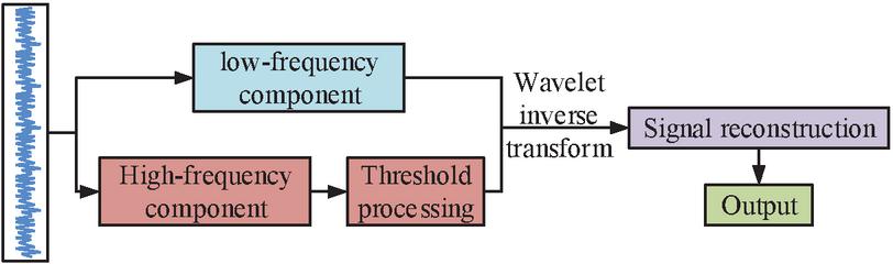
Figure 1 WT denoising process.
For time-series signals, WT can be classified into three types of wavelets, such as Haar wavelet, DbN wavelet and SymN wavelet, depending on the wavelet function [17–19]. In this study, the SymN wavelet was used for noise reduction of the raw data from the building ES. SymN wavelets are similar to DbN wavelets, but have better symmetry and are more beneficial for signal reconstruction. Where N denotes the order of the wavelet and N was taken to be 4 for this study. The research adopts Sym4 wavelet to reduce the noise of the original signal of the building electrical system. The selection of the wavelet basis is based on its symmetry: Compared with the DbN wavelet, the SymN wavelet has better symmetry, can effectively reduce the phase distortion during signal reconstruction, and is more conducive to preserving the timing information of the fault characteristics, which is crucial for fault diagnosis. After comprehensive evaluation, Sym4 was determined as the optimal order. SVM is a more widely used supervised machine learning algorithm. The main goal is to identify a hyperplane with a distribution of the various node types from the training samples at both ends and one that satisfies the minimal gap between the two ends [20]. As shown in Figure 2, SVM can classify linearly divisible data in two-dimensional space, where the red line is the best classification curve. The best classification curve becomes the best hyperplane if, in a higher dimensional space, the curve turns into a hyperplane. The support vector is the data that is closest to the best hyperplane.
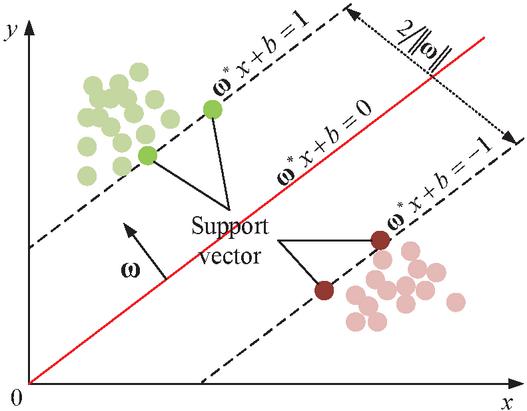
Figure 2 Principle of SVM classification in two dimensions.
Taking two-dimensional linearly divisible data as an example, assuming that the sample data is represented as , represents the input data and represents the data type, the hyperplane of this data can be represented by Equation (3).
| (3) |
and in Equation (3) denote the normal vector of the hyperplane and the distance from the hyperplane to the origin, respectively, where determines the direction of the hyperplane. The distance between the data and the hyperplane is denoted as B. The equation is given in Equation (4).
| (4) |
The optimal hyperplane for linearly divisible data is unique, both in terms of satisfying the conditions for the correct classification of the samples and in terms of making the differences between categories obvious. The search for the best hyperplane can therefore be transformed into a minimal problem optimization with constraints, which can be described by the computational procedure shown in Equation (5).
| (5) |
Equation (5) is the quadratic programming of the data samples. The Lagrange multiplier is introduced to improve Equation (5), and as demonstrated in Equation (6), the SVM’s decision function can be obtained.
| (6) |
is the decision function in Equation (6); represents the kernel function (KF) operation in SVM. The Gaussian kernel function (GKF) is currently the most used KF due to its advantages of strong localization and small computational effort.
| (7) |
In Equation (7) is the GKF and is the parameter that controls the local range of action. The Taylor series can be used to broaden the mapping process of the GKF, which is a monotonic function of the Euclidean distance between vectors. The GKF is employed in this study as the SVM’s KF. Figure 3 depicts the WT-SVM-based FD algorithm’s flow.
Figure 3 Flow of FD algorithm based on WT-SVM.
The collected building electrical fault signals are reconstructed with Sym4 wavelets for noise reduction and normalization, then fed into the SVM algorithm for training, the optimal KF parameters are determined by the cross-validation method, thresholds are set, and finally the fault classification and diagnosis results are derived.
3.2 Improved EFD Algorithm Combining CS and KNN
Since wavelet noise reduction performs poorly in high-dimensional data and the SVM algorithm is suitable for small data volumes, the performance of the algorithm does not improve in the face of large data volumes. As a result, the dimensionality of the fault data is reduced during the data pre-processing stage using CS, and the SVM is enhanced and the WT-SVM model is optimized using the KNN technique. With the goal to remove a significant number of unnecessary data and represent the necessary signal with a minimal amount of data, CS can benefit from the signal’s sparsity [21]. Its data processing process is shown in Figure 4.
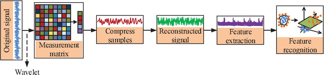
Figure 4 CS processing data flow.
Suppose the length of signal is , which can be represented by Equation (8) after scarification by a sparse matrix. Where is the orthogonal sparse matrix; and are the th transform basis vector and the sparse vector respectively.
| (8) |
The sparse vector is the transform coefficient of the signal on the sparse matrix. If the signal can be represented sparsely, the sparse vector s has finitely many non-zero values. After scarification of the signal, the signal is observed by projection through the observation matrix, and the observation result Y can be expressed by Equation (9).
| (9) |
in Equation (9) is the observation matrix satisfying . where is much smaller than . denotes the matrix consisting of the -dimensional observation vector obtained by observing the -dimensional signal with the -dimensional signal, i.e , . The whole CS process includes three steps: signal sparse representation, observed signal and signal reconstruction. The main methods of sparse representation include Fourier transform, WT and multi-scale geometric analysis, etc. In this study, WT is used for the sparse representation of the signal. Utilizing all of the data near each classification plane’s information is essential for improving SVM’s classification performance. The KNN classifier can make judgement on the data category by calculating the Euclidean distance from the data to be classified to each class of data, which can meet the requirements of SVM optimization [22]. Therefore, KNN is used to improve SVM and construct a new SVM-KNN algorithm. Suppose there are two classes of data, positive and negative, and the support vector representative points are denoted as and respectively, the data to be identified is , and the absolute value of the distance difference between and and is . Set the threshold . If , it means that is on the positive or negative side of the data and is far from the best hyperplane, and the data can be classified by SVM. If , it means that is near the best hyperplane, and it is easy to make mistakes if continue to classify by SVM. Therefore, in this case KNN needs to be used to calculate the distance to all support vectors. Figure 5 depicts the SVM-KNN algorithm’s classification concept and flow.
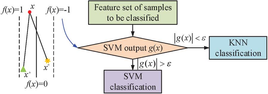
Figure 5 Classification idea and operation flow of SVM-KNN algorithm.
The data processed by CS and WT are input into SVM for training to get the optimal parameters. The data to be tested are pre-processed and input to the SVM to calculate . If , the result is output by the SVM; if , the classification result is input to the KNN. Since the input of KNN is SVM, the distance calculation equation used by KNN is not the commonly used Euclidean distance equation, but the equation modified by Equation (10).
| (10) |
Since this study uses a GKF whose kernel number satisfies , substitution gives Equation (11).
| (11) |
The Euclidean distance in the original input space is . Substituting this into Equation (11) shows that when and are greater than or equal to 0, for data samples and , is monotonically increasing about . In other words, there is no change in their relative positions and the only difference between the data in the feature space and the original input space is how close they are to each other. So, the two distance algorithms obtain exactly the same neighborhood data. It can also be seen that the classifier is to some extent independent of the KF parameters and has a more stable performance. After the algorithm completes the compressed sensing dimension reduction of the input signal, wavelet transform denoising, and classification diagnosis based on the improved support vector machine combined with K-nearest neighbors, the system not only outputs the specific fault type identification, but also generates structured maintenance decision support information. This information includes the possible location of the fault, the specific type of fault diagnosed and its confidence level, as well as the initial maintenance suggestions derived from the knowledge base or rule engine, such as isolation checks and withstand voltage tests for insulation breakdown of transformer windings, and the need to focus on checking the grounding resistance of relevant connection points for leakage of protective conductors, etc. These structured diagnostic results can be directly pushed to the building management system or maintenance management system platform, triggering the corresponding alarm mechanism, automatically generating maintenance work orders, and scheduling maintenance resources based on preset priority rules. The core processing flow of the CW-SVM-KNN fault diagnosis method proposed by the research institute has the adaptability to the electrical systems of different building types. Wavelet transform can effectively capture the key time-frequency characteristics of single-phase grounding faults and poor contact in residential buildings, as well as diverse faults in commercial buildings. Compressive sensing technology can flexibly handle different data scales ranging from simple residential systems to dense commercial sensor networks. The learning mechanism of the SVM-KNN classification framework focuses on the signal feature patterns themselves rather than the specific system topology. By integrating the training data covering typical fault samples of different buildings such as residential and commercial buildings, the model can establish extensive fault identification capabilities. Therefore, the universal design of the method makes its diagnostic performance mainly rely on the representativeness and coverage of the training data, and has the potential for application across building types.
4 Performance Evaluation of WT-SVMEFD Models Incorporating CS and KNN Algorithms
The study assessed the proposed WT-SVMFD model’s classification outcomes and investigated how data size affected the model’s precision. The performance of the algorithm improved by CS and K neighborhood was tested and the FD accuracy of the WT-SVM model before and after the improvement was compared and analysed.
4.1 Analysis of EFD Results Based on WT-SVM
A comprehensive low-voltage electrical tester was used to collect random fault signals from the building electrical experimental platform and noise reduction was applied to them by means of the Sym4 wavelet function. The fault types were set to 410 with a data volume of 400, and the variation of the model accuracy is shown in Figure 6.
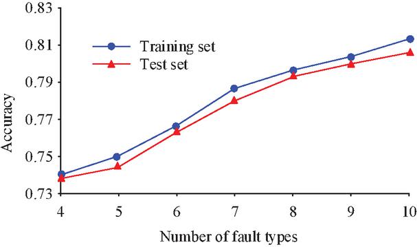
Figure 6 Variation of fault accuracy with type of fault.
As the number of defect categories rose for the same amount of sample data, as shown in Figure 6, the model’s accuracy increased for both the training and test sets. When there were 10 defect types, the model’s classification accuracy increased to 81.3% in the training set and 80.2% in the test set. This suggests that the model is more successful in categorizing WT-SVM with a wider variety of defects. To verify the effect of sample size on the classification effect of the WT-SVM model, the noise reduction data was divided into samples with data sizes of 400, 800, 1200, 1600, 2000 and 2400 and input into the model for training. The classification accuracy and training time consumed for the 10 fault types are shown in Figure 7.
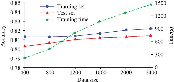
Figure 7 Volume of data versus accuracy and run time.
As demonstrated in Figure 7, the model accuracy increased as the sample data volume increased, but the trend was not readily apparent from the findings. The accuracy of the model training set and test set at 2400 data volume was 82.2% and 81.4% respectively, which was not much different from the accuracy of 400 data volume. The running time of the model was 257.3 s when the data volume was 400, while the running time was 1453.6 s when the data volume reached 2400, an increase of nearly 6 times. It is indicated that the signal features extracted after wavelet transform (Sym4, 5-layer decomposition) preprocessing only require a small amount of data to extract the key information sufficient to distinguish faults. The additional information brought by the newly added samples is limited, mainly manifested as the repetition or subtle variations of the existing features. It fails to effectively expand the discriminative information in the feature space, resulting in a bottleneck in the performance improvement of the model. It indicates that the research method has a relatively low data deployment requirement. Ten different building electrical fault types were identified at different data volumes and compared to a single SVM, Back Propagation (BP) neural network-based FD model, with the accuracy rates shown in Figure 8.
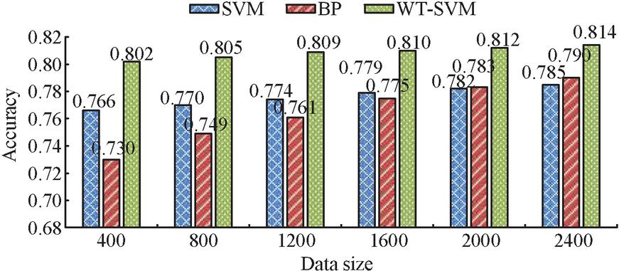
Figure 8 Classification accuracy of different algorithms.
Figure 8 demonstrates that for the same amount of data, the WT-SVM algorithm consistently outperformed the other two algorithms in terms of accuracy. At a data volume of 2400, the classification accuracy of the WT-SVM, SVM and BP algorithms for the test set was 81.4%, 78.5% and 79.0% respectively. This indicates that the WT-SVM algorithm can effectively diagnose building electrical faults. The accuracy exceeds that of SVM after the data reaches 2000. while the accuracy of WT-SVM and SVM is less affected by the change of data volume, indicating that the SVM series classifier is more advantageous in FD with fewer samples.
4.2 Evaluation of the Effectiveness of the Improved WT-SVMEFD Model Based on CS and KNN
The improved WT-SVMEFD model based on CS and KNN is denoted as CW-SVM-KNN. different number of nearest neighbors in the KNN algorithm will affect the experimental results to a large extent, so the -value needs to be determined first. The relationship between the size of the -values and the loss rate and accuracy rate is shown in Figure 9.
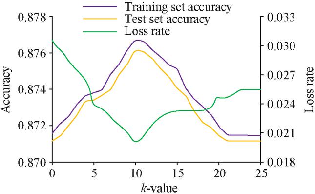
Figure 9 Effect of values on model loss rate and accuracy.
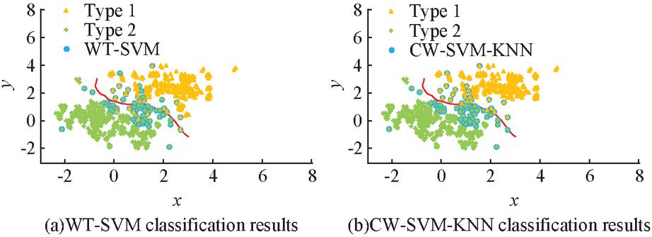
Figure 10 Classification results of the two models for fault data.
Figure 9 shows that as the value of rises, both the accuracy and the loss first rise and then fall until they reach their maximum values at the value of of 10, where the accuracy rate is the highest at 87.3% and the loss rate is the smallest at 1.9%. Figure 10 displays the classification outcomes for the WT-SVM and CW-SVM-KNN models after training with an 8:2 ratio between the training set and the test set.
Comparing Figures 10(a) and 10(b) it can be seen that the classification features of the two types of fault data are not particularly obvious, but the SVM can still find the best hyperplane by parameter training. It is evident in the WT-SVM algorithm that the SVM judges faults belonging to type 2 as type 1, while the CW-SVM-KNN model is able to classify faults more accurately, with almost no classification errors in the figure. To verify that the CW-SVM-KNN model can improve the accuracy of fault classification, 2400 fault data containing 10 types of faults were selected to train the CW-SVM-KNN, WT-SVM, and KNN algorithms, where the confusion matrix of CW-SVM-KNN is shown in Figure 11.
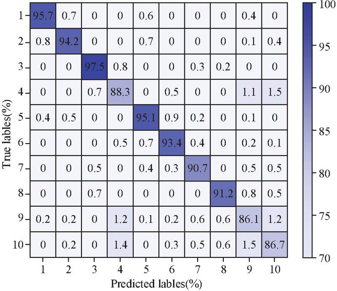
Figure 11 FD confusion matrix for CW-SVM-KNN model.
The numbers 1 to 10 in Figure 11 correspond in turn to the 10 fault types described in the previous section. The accuracy of the model is relatively low for the identification of three fault types: insulation breakdown of the winding in the transformer, damage to the insulator and leakage of the protective conductor. The model has a relatively low recognition accuracy rate for transformer winding insulation breakdown (Type 7), insulator damage (Type 9), and protective conductor leakage (Type 10). Quantitative analysis reveals that the fundamental reason lies in the high similarity of the characteristics of these three types of fault signals. The specific manifestations are as follows: The time-domain current waveforms of the transformer winding insulation breakdown and insulator damage faults both show significant high-frequency oscillation attenuation characteristics. The correlation coefficient of the time-domain waveforms of the two is as high as 0.72, indicating that their waveform forms are extremely close. At the frequency domain level, the energy entropy analysis based on five-layer wavelet decomposition shows that the average energy entropy values of the detail components of the fifth layer of the two types of faults differ slightly, only 2.4%, which are 3.82 and 3.91 respectively. Moreover, their main energies are highly concentrated in the 4.5–6.3 kHz frequency band, with an overlap rate as high as 89%. For the leakage fault of the protective conductor, the amplitude of the leakage current signal is too low, increasing by only about 18% on average compared with the normal state, and it is extremely easy to be submerged by background noise. Meanwhile, the difference range between the energy entropy of its wavelet detail component and the normal state is only between 5% and 8%, with insufficient discrimination. Further observation of the feature space distribution after dimensionality reduction by compressive sensing shows that the overlap rate of these three types of fault samples in the two-dimensional projection area reaches 40%, resulting in the difficulty for the support vector machine to establish a clear and effective classification boundary. The strong similarities shown in the time domain, frequency domain and feature space as mentioned above are the core reasons for the decline in the classification accuracy of the model for these three types of faults. The similarity of such features increases the classification difficulty, which can be achieved by enhancing high-frequency feature extraction or introducing temporal dynamic characteristic optimization algorithms. To further verify the performance of the research method, supplementary dynamic tests and large-scale data analysis are conducted, as shown in Table 1.
Table 1 Adaptability in dynamic environments
| Testing | |||
| Dimension | Condition Description | Key Metric | Result Value |
| Dynamic Environment | 30% load fluctuation | Diagnostic accuracy | 0.897 |
| Adaptability | Strong noise interference (SNR 0 dB) | Feature stability | Energy entropy variance 0.05 |
| Harmonic pollution (20% THD) | Key frequency band retention rate | 85% (4–6 kHz) | |
| Practical Application Efficiency | Real-time diagnosis in commercial buildings (8,400 samples/hour) | Average single-diagnosis delay | 18.3 milliseconds |
| Cross-scenario generalization (residential building data) | Accuracy | 0.883 | |
| Large-Scale | 100,000-sample training | Training time | 86 seconds |
| Data Processing | 1,000,000-sample online inference | Inference delay | 210 milliseconds |
| 1,000,000-sample processing | Memory consumption | 11.2 Gigabytes |
It can be seen from Table 1 that under voltage fluctuations of 30%, strong noise and harmonic interference, the accuracy rate of the research method remains 85%, because wavelet transform effectively separates fault characteristics, and compressive sensing retains the energy of key frequency bands. The research method was directly applied to the data of residential buildings, with an accuracy rate of 88.3%, proving that the model is insensitive to changes in building types. Meanwhile, the research method only takes 86 seconds to process 100,000 samples, with an online diagnosis delay of 210 ms for 1 million samples and a memory usage of only 11.2 GB. This further proves that the research method has good operational efficiency in large-scale data.
5 Conclusion
The security and dependability of building ES, which is a crucial component of contemporary residential buildings, are extremely vital to the tenants. The use of intelligent algorithms in FD technology offers a new assurance for the secure operation, repair, and upkeep of building electrics. A fault diagnosis method based on wavelet transform and SVM was designed in the research. The innovation lies in establishing a collaborative processing mechanism of compressive sensing and wavelet transform. Through joint noise reduction and feature compression, efficient preprocessing of signals is achieved while retaining the information of key frequency bands. Furthermore, an SVM-nearest neighbor dynamic optimization architecture is constructed. The nearest neighbor algorithm is utilized to correct the decision deviation of the support vector machine at the classification boundary in real time, thereby improving the discrimination accuracy of complex fault samples. The study’s findings demonstrated that the WT-SVM algorithm’s accuracy increased with the number of training fault types, however the size of the sample size had minimal bearing on the accuracy of the WT-SVM model. With a modest sample amount of data, the WT-SVM method was able to classify 10 fault types with an accuracy of 80.2%, and with a data size of 2400, it was able to do so with an accuracy of 81.4%, both of which were higher than the accuracy of using the SVM and BP algorithms separately. This shows that the WT-SVM algorithm can properly identify electrical issues in buildings while requiring less data. The CS and KNN algorithms significantly enhanced the CW-SVM-KNN model’s accuracy in finding faults, which resulted in a reduction in running time to 643.7 s. This suggests that using CS to lessen the dimensionality of the data can increase the model’s operational efficacy. This research hasn’t actually been implemented in a practical setting because it has only been done on an experimental platform to simulate and validate the suggested model. Investigating in-depth applications of this FD system for actual building electrical engineering should be the next stage.
Funding
The research is supported by Research Project on the Teaching Innovation Team of the Second Batch of National Vocational Education Teachers in 2021. Exploration and Practice of the Curriculum System for Integrating Intelligent Welding Technology with Professional (Industry) Standards. Subject No: ZI2021020203.
References
[1] Anbalagan T, Nath M K, Anbalagan A. Detection of atrial fibrillation from ECG signal using efficient feature selection and classification. Circuits, Systems, and Signal Processing, 2024, 43(9): 5782–5808.
[2] Darwish M M F, Hassan M H A, Abdel-Gawad N M K, Lehtonen M, Mansour D E A. A new technique for fault diagnosis in transformer insulating oil based on infrared spectroscopy measurements. High Voltage, 2024, 9(2): 319–335.
[3] Danjuma M U, Yusuf B, Yusuf I. Reliability, availability, maintainability, and dependability analysis of cold standby series-parallel system. Journal of Computational and Cognitive Engineering, 2022, 1(4): 193–200.
[4] John Y M, Sanusi A, Yusuf I, Modibbo U M. Reliability Analysis of Multi-Hardware-Software System with Failure Interaction. Journal of Computational and Cognitive Engineering, 2023, 2(1): 38–46.
[5] Xu B, Shen J, Liu S, Su Q, Zhang J. Research and Development of Electro-hydraulic Control Valves Oriented to Industry 4. 0: A Review. Chinese Journal of Mechanical Engineering, 2020, 33(2): 13–32.
[6] Niu G, Wang X, Golda M, Mastro S, Zhang B. An Optimized Adaptive PReLU-DBN for Rolling Element Bearing Fault Diagnosis. Neurocomputing, 2021, 445(20): 26–34.
[7] Zhang J, Zhang Q, He X, Sun G, Zhou D. Compound-Fault Diagnosis of Rotating Machinery: A Fused Imbalance Learning Method. IEEE Transactions on Control Systems Technology, 2021, 29(4): 1462–1474.
[8] Han Y, Ding N, Geng Z, Wang Z, Chu C. An optimized long short-term memory network-based fault diagnosis model for chemical processes. Journal of Process Control, 2020, 92(4): 161–168.
[9] Patil P S, Patil M S, Tamhankar S. Ensembles of Ensemble Machine Learning approach for Fault detection of Bearing. Solid State Technology, 2020, 63(6): 14442–14455.
[10] Chen J, Gao J, Jin Y, Zhu P, Zhang Q. Fault Diagnosis in Distributed Power-Generation Systems Using Wavelet Based Artificial Neural Network. European Journal of Electrical Engineering, 2021, 23(1): 53–59.
[11] Fu J, Leng T. Fault diagnosis and location method for electrical power supply and distribution of buildings. International Journal of Simulation and Process Modelling, 2020, 15(4): 333–342.
[12] Du T, Zhang H, Wang L. Analogue circuit fault diagnosis based on convolution neural network. Electronics Letters, 2019, 55(24): 1277–1279.
[13] Tuerxun W, Chang X, Hongyu G, Jin Z, Zhou H. Fault Diagnosis of Wind Turbines Based on a Support Vector Machine Optimized by the Sparrow Search Algorithm. IEEE Access, 2021, 9(1): 69307–69315.
[14] Zhang Y, Campana P E, Yang Y, Stridh B, Lundblad A, Yan J. Energy flexibility from the consumer: Integrating local electricity and heat supplies in a building. Applied Energy, 2018, 223(3): 430–442.
[15] Wang M H, Lu S D, Liao R M. Fault Diagnosis for Power Cables Based on Convolutional Neural Network with Chaotic System and Discrete Wavelet Transform. IEEE Transactions on Power Delivery, 2021, 37(1): 582–590.
[16] Soltani A A, Shahrtash S M. Decision tree-based method for optimum decomposition level determination in wavelet transform for noise reduction of partial discharge signals. IET Science, Measurement & Technology, 2020, 14(1): 9–16.
[17] Ertargin M, Yildirim O, Orhan A. Mechanical and electrical faults detection in induction motor across multiple sensors with CNN-LSTM deep learning model. Electrical Engineering, 2024, 106(6): 6941–6951.
[18] Xi Y, Chen Z, Tang X, Li Z, Zeng X. Type identification and time location of multiple power quality disturbances based on KF-ML-aided DBN. IET Generation, Transmission & Distribution, 2022, 16(8): 1552–1566.
[19] Peng F, Mu L, Fang C. Fault diagnosis of shipboard medium-voltage alternating current power system with fault recording data-driven SE-ResNet18-1 model. IEEJ Transactions on Electrical and Electronic Engineering, 2024, 19(3): 403–413.
[20] Kerboua A, Kelaiaia R. Fault diagnosis in an asynchronous motor using three-dimensional convolutional neural network. Arabian Journal for Science and Engineering, 2024, 49(3): 3467–3485.
[21] Wang X, Yang B, Wang Z, Lin Q, Chen C, Guan X. A compressed sensing and CNN-based method for fault diagnosis of photovoltaic inverters in edge computing scenarios. IET renewable power generation, 2022, 16(7): 1434–1444.
[22] Zheng S, Ding C. A group lasso based sparse KNN classifier. Pattern Recognition Letters, 2020, 131(1): 227–233.
Biography

Shukai Liu, an associate professor and master’s degree holder, serves as the leader of the electrical automation technology major at Changzhou vocational institute of engineering. He has been awarded the second prize of the National Teaching Achievement Award, is a candidate for the “Qinglan Project” for outstanding young backbone teachers in Jiangsu Province’s universities, holds the titles of Jiangsu Technical Expert, Jiangsu May 1st Innovation Expert, and Jiangsu Youth Job Expert, and is an excellent instructor in the National Vocational Education Skills Competition for the Machinery Industry. He has published over 20 academic papers in publicly issued journals both domestically and internationally, edited and co-edited 10 textbooks, and led and participated in 10 research projects at various levels.
Distributed Generation & Alternative Energy Journal, Vol. 40_5&6, 901–922.
doi: 10.13052/dgaej2156-3306.40561
© 2025 River Publishers