A New Representative Power Station Selection Method in Distributed Photovoltaic Cluster Power Forecasting
Wu Yidi1, Ma Xiaotian1, Li Mengyu1, Jiang Taoping2, Chen Ping1, Zhao Ruifeng1 and Hao Ying2
1State Grid Hebei Marketing Service Center, Shijiazhuang, China, 050035
2School of Automation, Beijing Information Science and Technology University, Beijing China, 100192
E-mail: bistufxyc2025@163.com
*Corresponding Author
Received 17 June 2025; Accepted 01 September 2025
Abstract
With the rapid development of distributed photovoltaic power generation systems, photovoltaic cluster power forecasting plays a vital role in the stable operation of power grids and optimal energy dispatching. Due to the large number of power stations in the PV cluster, wide distribution and high data dimension, it is not only computationally complex to directly predict all power stations, but also may reduce the forecasting accuracy due to data redundancy, so it is particularly important to reasonably select representative power stations in the cluster forecasting. In order to improve the accuracy of cluster forecasting, this paper proposes a new representative power station selection method based on vector error correction model (VECM), and uses spatiotemporal graph convolutional network to predict the power of distributed photovoltaic clusters. Firstly, a VECM is constructed, and the correlation between each power station and the cluster is analyzed by combining the results of variance decomposition method, and the power stations related to the cluster are selected as the representative power stations. Then, the heron optimization algorithm is introduced to calculate the optimal weight distribution of each representative power station. Finally, the spatiotemporal graph convolutional network is constructed by using the historical data of the representative power stations to realize the feature extraction of complex spatiotemporal data between photovoltaic power stations, and the power forecasting data of each representative power station is output, and the cluster forecasting power is obtained through the optimal weight calculation. An example is carried out in a distributed photovoltaic cluster in a province to prove the effectiveness of the proposed method in cluster forecasting.
Keywords: Photovoltaic power forecasting, distributed photovoltaic clusters, vector error correction model, spatial temporal graph convolutional network.
1 Introduction
Photovoltaic power generation technology is considered one of the most promising new energy sources because of its high efficiency and direct conversion of solar energy into electricity without producing any pollutants [1–4]. In recent years, driven by the goals of “carbon peak” and “carbon neutrality”, China’s photovoltaic industry has developed rapidly [5, 6]. Due to the scattered solar energy resources and low energy density, photovoltaic power generation is naturally suitable for distributed power generation mode.
In addition, the distribution of wasteland resources and electricity load in China is extremely uneven, and distributed photovoltaic power generation will be the optimal form of large-scale photovoltaic application [7]. Distributed photovoltaic power generation is distributed, intermittent, and fluctuating, and its power generation is greatly affected by weather, seasonal, and diurnal changes, which makes it difficult to predict and manage the power output of a single photovoltaic power station, which increases the difficulty of grid dispatching and stable operation [8, 9]. However, the output of distributed photovoltaic clusters has better regularity than that of a single distributed generation system, which greatly improves the accuracy of power forecasting of distributed photovoltaic power generation and reduces the difficulty of power forecasting, so it is particularly important to carry out cluster forecasting [10].
Current research has focused on forecasting using time-series-based methods, however, PV sites located in similar geographic and climatic environments often exhibit similar power variations at the same time points due to the spatial correlation of distributed PV systems. This means that there is a certain correlation between the historical power of each station and the future power of neighboring stations, which is a spatiotemporal correlation [11]. Literature [12], a graph convolutional neural network was used to extract spatial features, and a multi-layer modal subsequence that could reflect the temporal change characteristics of historical data was constructed by using a graph convolutional neural network to extract spatial features, and a bidirectional long short-term memory neural network was used to predict the power of photovoltaic power generation. In [13], an ultra-short-term photovoltaic output forecasting method based on graph convolutional neural network and long short-term memory network (GCN-LSTM) was proposed, in which the graph convolutional neural network was used to extract the spatial features of the graph model, and the time series information containing the spatial features was obtained, and finally the time series data was input into the long short-term memory network for photovoltaic output forecasting. Literature [14], a combined forecasting model based on the fusion of temporal features and spatial relationships was proposed, in which multiple LSTM sub-models were used to extract the temporal features, and the natural gradient enhancement (NGBoost) algorithm was used for ensemble learning, then the meteorological parameters were analyzed and the spatial features were extracted by two-dimensional convolutional neural network (2D-CNN) for spatial correlation forecasting, and finally the advantages of the two forecasting models were integrated to construct a spatiotemporal information combination forecasting model. Most of the above methods adopt the method of combined forecasting, and model the temporal and spatial features separately, which lacks the ability to deeply integrate the two. Therefore, this paper uses a spatiotemporal graph convolutional network, considers the evolution of nodes in time series and the spatial relationship between nodes, captures the feature information in time and space, and effectively integrates them together for learning and forecasting, so as to capture the complex spatiotemporal correlation between photovoltaic power plants.
In cluster power forecasting, the selection of representative power stations is crucial. If the selected representative power station is not typical and cannot represent the entire cluster, the forecasting accuracy of the cluster cannot be guaranteed, even if the forecasting accuracy of the representative power station is high. Therefore, it is crucial to select representative power stations that are highly correlated with cluster power to improve the forecasting accuracy. Literature [15], the Pearson correlation coefficient was used as the evaluation index to select representative power stations, and the weight coefficient representing the electric field was the ratio of the sum of the installed capacity of the cluster to the installed capacity of the representative wind farm. In [16], the photovoltaic power stations with high correlation of cluster output power and high power forecasting accuracy were taken as representative power stations, and the weight coefficients of each representative photovoltaic power station were calculated by mathematical statistical methods. At present, the selection of representative power stations usually relies on simple statistical indicators, such as Pearson correlation coefficient or other screening methods based on correlation and power forecasting accuracy, which mostly rely on short-term and linear relationships, and ignore the possible long-term cointegration relationship or dynamic adjustment effect between power stations and clusters. Literature [17] analyzes the dynamic relationship between water resource utilization and economic growth in China by constructing a VECM between total water use and GDP. In [18], a VECM of battery clusters and battery cells was constructed based on random voltage fragment data, and the dynamic influence of battery cells on battery clusters was analyzed. Literature [19] uses the VECM to analyze the interaction mechanism between multiple industrial industries, quantitatively characterize the complex coupling relationship between industrial industries, and realize the accurate forecasting of the load of industrial industries. The above literature uses the VECM to analyze the long-term and short-term relationships between variables at the same time, and reflects the dynamic change law between variables. Therefore, this paper uses VECM and variance decomposition to select cluster-representative power stations.
In this paper, we propose a new representative power station selection method based on VECM, and use Spatio-Temporal Graph Convolutional Networks (STGCN) to predict the power of distributed photovoltaic clusters. Firstly, the VECM model was constructed, and the correlation between each power station and the cluster was analyzed by combining the results of variance decomposition method, and the power stations related to the cluster were selected as the representative power stations. Then, the Secretary bird optimization algorithm (SBOA) [20] was introduced to determine the weights of each representative power station. Finally, the STGCN model is constructed by using the historical data of the representative power stations to realize the feature extraction of complex spatio-temporal data between photovoltaic power stations, and the power forecasting data of each representative power station is output, and the cluster forecasting power is obtained through the optimal weight calculation. An example is carried out in a distributed photovoltaic cluster in a province to prove the effectiveness of the proposed method in cluster forecasting.
2 Representative Power Station Selection and Weight Calculation
2.1 Vector Error Correction Model
The VECM is an econometric model for non-stationary time series analysis, which is mainly used to study the long-term equilibrium relationship and short-term dynamic adjustment between multiple time series variables. VECM is an extension of the vector autoregressive model (VAR), which introduces cointegration analysis and error correction terms, so that VECM can capture both short-term fluctuations and the influence of long-term relationships, so as to solve the problem of ignoring cointegration relations when processing non-stationary time series data in VAR models, and is suitable for variables with cointegration relationships.
The mathematical form of VECM is as follows [21]: Remembering time series vectors , each component is a time series, and when selected to represent a power station, it can be a power series for each plant and the entire cluster. For linear regression, the VAR model can be obtained, and its expression is:
| (1) |
where is the model variable; is the p-order hysteresis of the model variable.
Performing a differential transformation on Equation (1) yields:
| (2) |
where: , where is a matrix of adjustment coefficients, each of which corresponds to a set of weights of a cointegration combination, is a cointegration vector matrix, and each row vector is a cointegration vector; can be expressed as , and since is an error correction term , the general expression of VECM can be obtained as:
| (3) |
The error correction term reflects the long-term equilibrium relationship between the variables, and the coefficient matrix reflects the adjustment speed of the error correction term to the equilibrium state when the equilibrium relationship between the variables deviates from the long-term equilibrium state. The coefficient of the difference term of the independent variable reflects the effect of short-term fluctuations of each variable on the short-term change of the dependent variable [22].
2.2 Variance Decomposition Method
According to the above analysis, it can be seen that the correlation between each power station and the cluster is mainly affected by three parameters, namely . For these three parameters, the variance decomposition method is usually used in VECM to reassemble the information of the three parameters to extract the key information. The variance decomposition method quantifies the impact of different factors on overall fluctuations by breaking down the overall fluctuation (variance) of a complex variable into the contributions of its individual components.
For Equation (3), transform it and introduce the lag operator , available:
| (4) |
The result is:
| (5) |
Where is a k-order lag operator; is the identity matrix.
If the model corresponding to Equation (5) is stationary, then it can be expressed as an infinite moving average process of the white noise vector, namely:
| (6) |
where is the coefficient matrix, which represents the degree of influence of the first-order hysteresis white noise vector on , .
The corresponding component form of Equation (6) is as follows:
| (7) |
where is the specific element of the coefficient matrix , which means the influence of the th component of the k-order lag perturbation vector on .
Under the premise that the components of are not sequence-related and the covariance matrix is a diagonal matrix, the variance of is:
| (8) |
Where is the variance of the th variable.
The variance of can be decomposed into n uncorrelated influencing components, and the influence of the th variable on the th variable can be observed according to the relative contribution rate of the variance to the variance based on the impact of the variable , that is, the quantitative analysis of the correlation between each power station and cluster can be realized by calculating the size of . is calculated as shown in Equation (9):
| (9) |
2.3 Selection Method of Representative Power Station Based on VECM Model
The representative power station selection method based on the VECM model is as follows: firstly, the stationarity test of the power series of each power station and cluster is carried out, and if there is an unstationary sequence, the difference method is used to keep each power series of the same order single whole. Then, under the condition of ensuring the stability of each power series, the results of Akaike information criterion (AIC), Schwarz information criterion (SIC) and Hannan-Quinn criterion (HQ) were comprehensively evaluated to determine the optimal lag order of the model. Then, the Johansen test is used to test the cointegration relationship between power sequences. Then, according to the analysis results of the above steps, the VECM model was established, and the correlation between each power station and the cluster was analyzed by combining the results of variance decomposition method, and the power stations related to the cluster were selected as the representative power stations. Figure 1 shows the framework of the representative power plant selection method based on the VECM model.
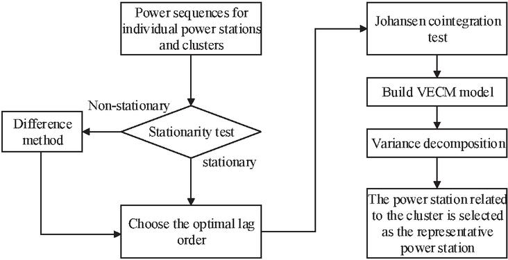
Figure 1 Framework of representative power station selection method based on VECM model.
2.4 Calculation of the Weights of Representative Power Stations Based on SBOA
The Secretary Bird Optimization Algorithm is a novel meta-heuristic algorithm inspired by the hunting and avoidance behavior of the secretary bird. SBOA excels in optimization problems due to its powerful global search capabilities, dynamic adjustment capabilities, and fast convergence characteristics. By simulating the predation and escape strategies of the secretary bird, SBOA can effectively avoid falling into the local optimal and ensure that the global optimal solution is found. In addition, the SBOA algorithm has a simple structure and is easy to implement, which is suitable for various complex nonlinear and multi-peak optimization problems. These advantages enable SBOA to provide efficient and accurate solutions in practical applications.
The specific process of using SBOA to calculate the weights of representative power stations is as follows: first, a fitness function is defined as the square error, that is, the square of the difference between each representative power station and its corresponding weights and cluster power, which is used to evaluate the forecasting error of different weight combinations. Then, the algorithm parameters are initialized to generate the initial population position according to Equation (10).
| (10) |
where denotes the position of the th secretary bird; and are the lower and upper bounds, respectively; is a random number between 0 and 1; Dim is the dimension of the problem variable.
Then, in each iteration, according to the search strategy of the SBOA, during the exploration phase, the location is continuously updated by simulating the hunting behavior of the secretary bird. The exploratory phase consists of three stages:
In the first stage, the position of the prey was updated and mathematically modeled using Equation (11).
| (11) |
Where is the current number of iterations; is the maximum number of iterations; is the value of its th dimension; and are the stochastic candidate solutions for the first iteration. is a randomly generated array of dimensions of in the interval [0, 1].
In the second stage, the position of the consumed prey is updated mathematically using Equations (12)–(13).
| (12) | |
| (13) |
where is an array of of dimension randomly generated from the standard normal distribution; is the current optimal value.
The third stage of attacking the prey position is updated mathematically using Equations (14)–(17).
| (14) | |
| (15) | |
| (16) | |
| (17) |
where is the nonlinear perturbation factor; denotes the Levy flight distribution function; s is 0.01, is 1.5, u and v are random numbers in the interval [0,1]. is the gamma function.
The location update for the Exploration stage is represented as:
| (18) |
where is the new state of the th secretary bird in the exploration stage; is the fitness value of its objective function.
Then it enters the escape stage, simulates evasion behavior, finely searches for and further updates the location in the promising area, calculates new fitness values, and records and updates the current optimal weight combination. The escape stage consists of two escape strategies, which are mathematically modeled as follows:
| (19) | |
| (20) |
where corresponds to the strategy of using environmental camouflage; corresponds to the strategy of direct escape; rand is 0.5, and is an array with a dimension of randomly generated from the normal distribution. is a random candidate solution for the current iteration; is a random number with an integer of 1 or 2; is a random number that is randomly generated between (0,1).
The location update of the escape stage is represented as:
| (21) |
where is the new state of the th secretary bird in the escape stage; is the fitness value of its objective function.
After several iterations, the algorithm finally outputs the optimal weight combination of representative power stations. The algorithm flow chart is shown in Figure 2.
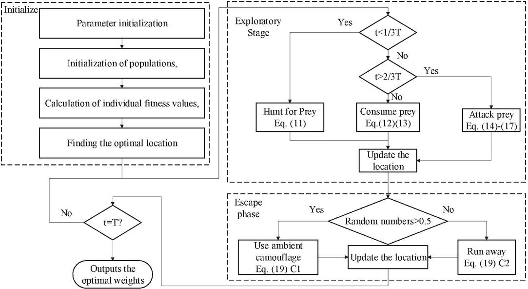
Figure 2 Flow chart of the SBOA algorithm.
3 Spatiotemporal Graph Convolutional Networks
STGCN effectively captures the spatiotemporal dependencies in the data by performing spatiotemporal convolution operations on the graph structure. It represents the spatio-temporal data as a graph structure, aggregates and updates the features of nodes and their neighbors through spatial convolution, and captures the temporal features by using temporal convolution, which can flexibly process graph structure data and carry out in-depth feature extraction, and has powerful spatio-temporal modeling capabilities. For the power data of photovoltaic power plant clusters with obvious spatiotemporal correlation, it is difficult for traditional forecasting methods to effectively capture this complex spatiotemporal relationship, but STGCN can improve the accuracy and reliability of forecasting through its powerful spatiotemporal feature extraction ability.
In STGCN, the power data of PV power plants is organized into a graph, where nodes represent different PV plants and edges represent the spatial relationships between power stations. The spatial relationship between power stations is quantified by using the adjacency matrix constructed by the geographical location information of the power station, and the adjacency matrix is defined as:
| (22) | ||
| (23) |
where is the geographical distance between the photovoltaic power station and ; is the variance of the distance of the photovoltaic power station; is the distance threshold; is latitude, in radians; is the longitude, in radians; is the radius of the earth, which is usually taken as 6371 km.
The STGCN model includes two spatiotemporal convolution modules, and each spatiotemporal convolution module contains two temporal convolution blocks and spatial convolution blocks. The time convolution block first performs a convolution operation, which regards the time dimension as the width of the image and the number of nodes as the height of the image, and uses the convolution kernel to slide in the time dimension to extract the time features. Secondly, a gating mechanism similar to the Gated Linear Unit (GLU) is used to adjust the influence of different convolution results. Finally, the gating results are combined with the convolution results to extract the time features. The spatial convolutional block uses the adjacency matrix to perform a weighted sum of the temporal features of each node, and fuses the features of each node with the features of its neighbors, effectively capturing the spatial correlation between nodes. The calculation process is shown in Figure 3.
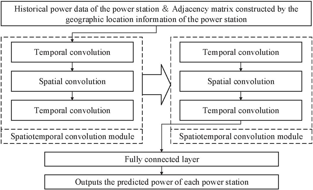
Figure 3 Structure of STGCN.
4 Overall Forecast Framework
According to the principle of the above method, a cluster power forecasting model considering the spatiotemporal correlation characteristics of distributed photovoltaic power stations is constructed, and the overall process of the forecasting model is shown in Figure 4, which is divided into three parts, namely the selection of representative power stations based on the VECM model, the weight calculation of representative power stations based on the secretary bird optimization algorithm, and the cluster power forecasting based on the spatiotemporal graph convolution model. The calculation steps for the model are as follows:
(1) Data preprocessing: preprocess the historical power data of each power station, remove outliers, and fill in the missing data.
(2) Selection of representative power stations: The stationarity test of the preprocessed historical power data is carried out, and the optimal lag order of the model is determined under the condition of ensuring the stability of each power series. Then, the Johansen test was used to test the cointegration relationship. Finally, the VECM model is constructed, and the correlation between each power station and the cluster is analyzed by combining the results of variance decomposition method, and the power stations related to the cluster are selected as the representative power stations.
(3) Weight calculation: The selected historical power data of the representative power station and the historical power data of the cluster are input into the Egret optimization algorithm to calculate the optimal weight value of the representative power station.
(4) Calculate the adjacency matrix: calculate the adjacency matrix according to the geographical location information of the power station.
(5) Power forecasting: The spatiotemporal graph convolution model is used to input the historical power data of the representative power station and the corresponding adjacency matrix to obtain the predicted power of each representative power station.
(6) Cluster power calculation: the sum of the predicted power of each representative power station multiplied by the corresponding weight is the cluster predicted power.
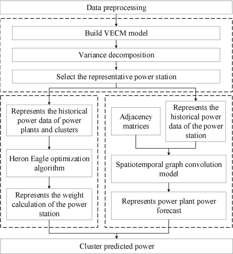
Figure 4 Predictive model flow.
5 Case Analysis
5.1 Data Description
In this paper, ten distributed photovoltaic power stations with good data quality were selected from a distributed photovoltaic power station cluster in a certain province, and the maximum power of the ten power stations was 777.9 kW, and the time was from January 1, 2021 to December 31, 2021, with a time resolution of 15 minutes.
5.2 Evaluation Indicators
The Mean Absolute Error (MAE) and Root Mean Square Error (RMSE) are selected as the evaluation indexes for PV power forecasting. The formula for calculating MAE and RMSE are as follows:
| (24) | |
| (25) |
where is the total number of samples; is the true value of the th sample; is the predicted value of the th sample; is the installed capacity of the power station.
5.3 Representative Power Station Selection and Weight Calculation
First, the data is preprocessed, and the missing and abnormal data is populated. Due to the large gap in the data of each power station. Therefore, logarithmic processing is carried out on the data to narrow the gap between the power data of different power stations.
ADF test was performed on the data. The test results are shown in Table 1. As can be seen from Table 1, the stationarity test results of each power station and cluster power series are all “Yes”, indicating that these power sequences are stationary and do not need to be differentiated to proceed with the next steps.
Table 1 Test results of power sequence stationarity
| Power Station | ADF Statistic | p-value | Smooth or Not |
| 1 | -71.6364 | 0 | Yes |
| 2 | -84.2071 | 0 | Yes |
| 3 | -74.7693 | 0 | Yes |
| 4 | -78.9767 | 0 | Yes |
| 5 | -76.86 | 0 | Yes |
| 6 | -73.8572 | 0 | Yes |
| 7 | -84.7832 | 0 | Yes |
| 8 | -81.9862 | 0 | Yes |
| 9 | -82.3449 | 0 | Yes |
| 10 | -70.6854 | 0 | Yes |
| ALL | -89.6796 | 0 | Yes |
A general VAR model was established, and the optimal lag order of the model was determined to be 97 by using the AIC criterion, SIC criterion and HQ criterion. The Johansen cointegration test was performed on the power sequences, and the test results are shown in Table 2. As can be seen from Table 2, the data has a cointegration relationship, which satisfies the basic conditions for building VECM, and the model can be constructed.
Table 2 Results of Johansen’s cointegration test
| Trace | 5% Critical | Max Eigen | 5% Critical | |
| Rank (r) | Statistic | Value (Trace) | Statistic | Value (Max Eigen) |
| 0* | 10145.2 | 306.8988 | 1771.154 | 73.9355 |
| 1* | 8374.05 | 259.0267 | 1154.687 | 67.904 |
| 2* | 7219.363 | 215.1268 | 1004.612 | 61.8051 |
| 3* | 6214.751 | 175.1584 | 1001.905 | 55.7302 |
| 4* | 5212.846 | 139.278 | 914.3666 | 49.5875 |
| 5* | 4298.48 | 107.3429 | 838.8558 | 43.4183 |
| 6* | 3459.624 | 79.3422 | 768.4958 | 37.1646 |
| 7* | 2691.128 | 55.2459 | 741.3553 | 30.8151 |
| 8* | 1949.773 | 35.0116 | 681.1245 | 24.2522 |
| 9* | 1268.648 | 18.3985 | 650.9736 | 17.1481 |
| 10* | 617.6748 | 3.8415 | 617.6748 | 3.8415 |
| Note: * indicates significant at the 5% significance level. | ||||
The VECM model was constructed, and the variance decomposition of the constructed VECM error term was performed, and the specific results of variance decomposition of cluster power are shown in Figure 5. As can be seen from Figure 5, in addition to the cluster power itself, the power stations that contribute more to the cluster power are power station 1, 2, 3, 6, and 7, so these five power stations are selected as representative power stations, and then SBOA is used to calculate the weight of each representative power station, and the best weight coefficients are obtained: 2.0075, 1.419, 3.2625, 2.5212, 2.5234, and finally the cluster predicted power calculation formula is as follows:
| (26) |
where is the predicted power of the cluster; , and are the predicted power of power station 1, 2, 3, 6, and 7, respectively.
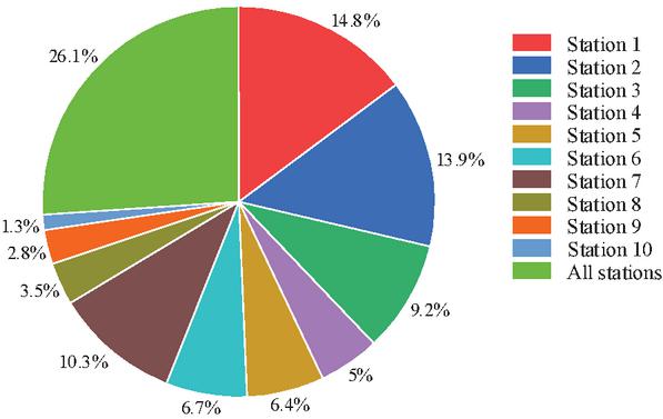
Figure 5 Variance decomposition results.
Compared with the VECM model, the representative power stations are selected based on the maximum correlation-minimum redundancy feature selection method, and the representative power stations are obtained as power stations 6, 8, 7, 9 and 5, and then the weights of each representative power station are 2.4376, 1.8956, 1.5068, 2.4855 and 1.8273 respectively, and the final formula for calculating the predicted power of the cluster is as follows:
| (27) |
where is the predicted power of the cluster; , and are the predicted power of power stations 6, 8, 7, 9, and 5, respectively.
5.4 Analysis of Forecast Results
This paper proposes four cluster power prediction methods for comparison: method 1 uses the VECM model to select the representative power stations, calculates the weights of each representative power station through SBOA, and uses STGCN to predict the power of the representative power stations and weights the sum; Method 2: Directly use the STGCN model to predict and sum the power of all power stations; Method 3 is similar to Method 1, which uses the maximum correlation-minimum redundancy method to select representative power stations; Method 4 is similar to Method 1, but uses the BiLSTM model instead of STGCN for forecasting.
The forecasting results are shown in Table 3, and the forecasting curve is shown in Figure 6.
| Method | MAE/% | RMSE/% |
| 1 | 1.94 | 2.80 |
| 2 | 2.77 | 3.11 |
| 3 | 2.48 | 3.22 |
| 4 | 3.53 | 7.02 |
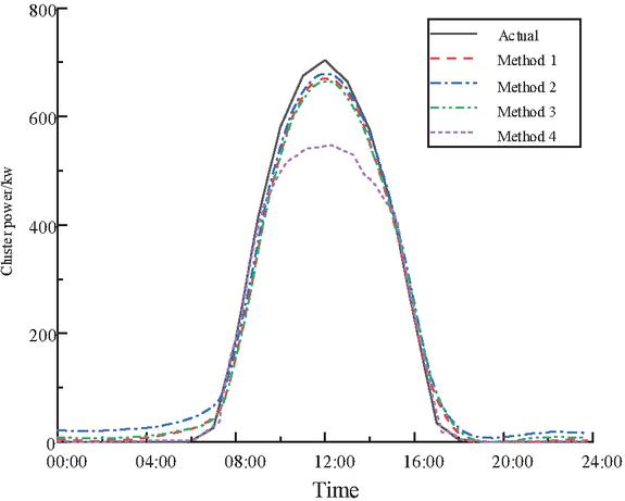
Figure 6 Forecasting curve.
In Figure 7, comparing the MAE, MSE, RMSE and MAPE values of the four methods, the comprehensive index of method 1 is stronger than that of the other methods, among which, MAE, MSE and RMSE are significantly lower than those of the other methods, and the MAPE ratio is much lower than that of method 4 and slightly higher than that of methods 2 and 3, which shows that the prediction results of method 1 are significantly stronger than those of the other three methods, and the prediction accuracy is higher.
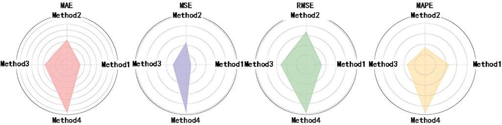
Figure 7 Error analysis diagram.
Compared with method 1 and method 2, the MAE and RMSE of all power stations are 2.77% and 3.11%, respectively, and the MAE and RMSE of data representing power stations are 1.94% and 2.80%, respectively, and the results show that the method of inputting data representing power stations to predict the cluster power is better. This difference suggests that although the spatial relationship between all power stations is preserved, the importance of the power stations cannot be distinguished, which may introduce redundant information and even noise, which may affect the forecasting accuracy. However, the forecasting after selecting the representative power station can reduce the data input dimension, make the model calculation more efficient, and avoid the interference of low correlation or noisy power stations on the forecasting results, and improve the accuracy of cluster power forecasting.
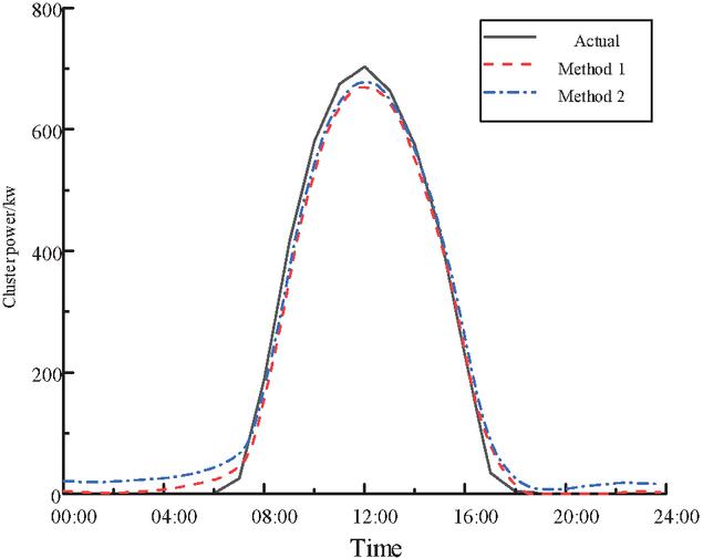
Figure 8 Comparison of forecasting curves of method 1 and method 2.
Compared with the forecasting results of Method 1 and Method 3, the forecasting accuracy of representative power stations selected based on the VECM model is higher. Method 3 uses the mRMR method to select representative power stations, although it can reduce the redundancy information, it only focuses on the selection of the most correlated and least redundant power stations, and ignores the influence of long-term cointegration relationship. In contrast, the VECM model used in Method 1 can identify the cointegration relationship between each power station and the cluster, capture their long-term correlation, and reveal the dynamic adjustment process of power station power to cluster power in the short term, so as to ensure that the selection of representative power stations is more reasonable and accurate, and improve the forecasting accuracy of the cluster.
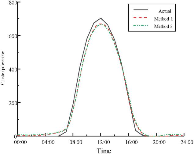
Figure 9 Comparison of forecasting curves of method 1 and method 3.
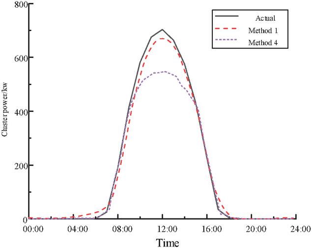
Figure 10 Comparison of forecasting curves of method 1 and method 4.
Compared with method 1 and method 4, method 1 uses the STGCN model for forecasting and method 4 uses the BiLSTM model for forecasting, and the results show that the forecasting error of the cluster power predicted by the STGCN model is smaller. The STGCN model can model the spatial dependence and time series characteristics of power station power data at the same time, effectively capture the spatiotemporal correlation between power stations, and make more accurate forecastings. Although the BiLSTM model can capture the two-way time series dependencies and has strong ability to model time series, it cannot capture the spatial correlation between power stations and can only rely on the time dimension for forecasting, resulting in incomplete forecasting information, so the forecasting error is larger than that of the STGCN model.
6 Conclusion
In this paper, a new method for selecting representative power stations based on VECM model is proposed, and then the weight of each representative power station is calculated by using the Egret optimization algorithm, and finally the power forecasting is carried out by using the STGCN model. Taking a distributed photovoltaic cluster in a province as an example, this paper analyzes the power forecasting method of distributed photovoltaic cluster, and obtains the following conclusions:
(1) The STGCN model can effectively capture the spatiotemporal correlation between photovoltaic power stations and improve the forecasting accuracy of cluster power.
(2) Reasonable selection of representative power stations for forecasting can effectively remove redundant information, reduce data dimensions, improve the representativeness of data input, and improve forecasting performance;
(3) The method of selecting representative power stations by using the VECM model proposed in this paper can not only reveal the long-term equilibrium relationship between each power station and the cluster power, but also capture the dynamic adjustment of the power of each power station to the cluster power in the short term, so as to ensure that the selection of representative power stations is more reasonable and reliable.
The historical power data of photovoltaic power stations are mainly used for forecasting, and meteorological factors can be considered as auxiliary characteristics in future research to further improve the accuracy of power forecasting of photovoltaic clusters.
Acknowledgment
Science and Technology Project of State Grid Hebei Electric Power Co., Ltd.: Research on Multi-load Feature Identification, Analysis and Prediction Technology in the Context of Rural Revitalization (Project No.: KJ2024-034).
References
[1] TIAN Zheng-qing, ZHANG Yong, LIU Xiang, et al. Effects of Photovoltaic Power Station Construction on Terrestrial Environment: Retrospect and Prospect [J]. Environmental Science, 2024, 45(01):239–247.
[2] Niu, X., and Luo, X. (2023). Policies and Economic Efficiency for Distributed Photovoltaic and Energy Storage Industry. Distributed Generation & Alternative Energy Journal, 38(04), 1197–1222.
[3] Zheng Wanting, Xiao Hao, Pei Wei. Probabilistic power forecasting for regional distributed photovoltaic systems using NGBoost and enhanced weight optimization[J]. Distribution & Utilization, 2024, 41(07):19–28.
[4] Zhou Yi, Xiao Xianyong, Zhao Qinghua, et al. Photovoltaic power forecasting based on combined data cleaning and improved attention mechanism[J]. Distribution & Utilization, 2024, 41(10):31–37+49.
[5] Li Ye, Influence of Accessed Distributed Photovoltaic Power Generation on Power Quality of Distribution Network[J]. Popular Utilization of Electricity, 2024, 39(03): 35–36.
[6] He Yihui, Guan Lin, Wang Tong, et al. Quantitative Evaluation and Analysis of the Planning and Construction of the New Power System in China Southern Power Grid[J]. Southern Power System Technology, 2024, 18(10): 40–53.
[7] Wang Wenjing, Wang Sicheng. Status and Prospect of Chinese Distributed Photovoltaic Power Generation System[J]. Bulletin of Chinese Academy of Sciences, 2016, 31(02): 165–172.
[8] Xu, Z., Xiang, K., Wang, B., and Li, X. (2024). Study on PV Power Prediction Based on VMD-IGWO-LSTM. Distributed Generation & Alternative Energy Journal, 39(03), 507–530.
[9] Li, H., Li, Z., Wang, C., Xia, L., Tan, H., and Li, K. (2024). Based on Deep Learning Model and Flink Streaming Computing Short Term Photovoltaic Power Generation Prediction for Suburban Distribution Network. Distributed Generation & Alternative Energy Journal, 39(04), 789–806.
[10] Zheng Xiaoyu, Ji Yu, Zhang Ying, et al. Coordinated Optimal Control of Distributed Photovoltaic Cluster Based on Model Predictive Control [J]. Power System and Clean Energy, 2019, 35(07):66–74.
[11] Boussif O, Boukachab G, Assouline D, et al. Improving day-ahead Solar Irradiance Time Series Forecasting by Leveraging Spatio-Temporal Context[J]. Advances in Neural Information Processing Systems, 2024, 36.
[12] Li Hao, Ma Gang, Li Tianyu, et al. Hybrid Model for Short-term Photovoltaic Output Prediction Based on Spatiotemporal Correlation[J]. Proceedings of the CSU-EPSA, 2024, 36(05):121–129.
[13] Han Xiao, Wang Tao, Wei Xiaoguang, et al. Ultrashort-term photovoltaic output forecasting considering spatiotemporal correlation between arrays[J]. Power System Protection and Control, 2024, 52(14):82–94.
[14] Yang X, Zhao Z, Peng Y, et al. Research on distributed photovoltaic power prediction based on spatiotemporal information ensemble method[J]. Journal of Renewable and Sustainable Energy, 2023, 15(3).
[15] Wang Youjia, Lu Zongxiang, Qiao Ying, et al. Short-Term Regional Wind Power Statistical Upscaling Forecasting Based on Feature Clusterin [J]. Power System Technolo, 2017, 41(05):1383–1389.
[16] Chen Ying, Chen Fugui, Chen Xu, et al. The regional photovoltaic power forecasting method based on statistical up-scaling approach[J]. Renewable Energy Resources, 2012, 30(11):20–23.
[17] Song Yang, Chen Chen. Study on the relationship between water resources utilization and economic growth based on VECM model[J]. Yellow River, 2022, 44(S2):52–54
[18] Guo Yuan, Xia Xiangyang, Yue Jiahui, et al. Battery Cluster Inconsistency Detection Method and Intelligent O&M Scheme Based on Vector Error Correction Model[J]. Electric Power, 2024, 57(06):9–17+44.
[19] Guo Yaoyang, Zhang Li, Wei Yusi, et al. Research on Electricity Load Forecasting Technique Considering Inter-industry Coupling and Correlation Characteristics[J]. Electric Power Information and Communication Technology, 2025, 23(02):1–10.
[20] Fu Y, Liu D, Chen J, et al. Secretary bird optimization algorithm: a new metaheuristic for solving global optimization problems[J]. Artificial Intelligence Review, 2024, 57(5):1–102.
[21] Xiang Yubo. Impact Factor of Chinese Carbon Emission Allowance Price, Based on Cointegration Test and VECM [D]. Shanghai: Shanghai University Of Finance and Economics, 2022.
[22] Tian Wenfuhui. The dynamic relationship between energy con-sumption and economic growth in Yunnan: An empirical study based on the vector error correction model[J]. Science Technology and Industry, 2022, 22(1):295–302 (in Chinese).
Biographies
Wu Yidi graduated from Huazhong University of Science and Technology with a bachelor’s degree in electrical engineering and automation, and is now working in the marketing service center of State Grid Hebei Electric Power Co., Ltd., a senior engineer, with the main research direction of electricity forecasting, electricity information collection, electricity market and electricity tariff.
Ma Xiaotian graduated from the School of Science and Technology of North China Electric Power University, majoring in electrical engineering and automation, with a bachelor’s degree, and is now working in the marketing service center of State Grid Hebei Electric Power Co., Ltd., a senior engineer, whose main research direction is agency power purchase and electricity forecasting.
Li Mengyu graduated from Hebei University of Technology with a master’s degree, and is now working in the digital room of technology development in the marketing service center of State Grid Hebei Electric Power Co., Ltd., with the main research direction: power data analysis and artificial intelligence technology application.
Jiang Taoping graduated from Jiangxi University of Science and Technology with a bachelor’s degree in automation, and is now studying at Beijing Information Science and Technology University, with a research direction of photovoltaic forecasting.
Chen Ping graduated from North China Electric Power University with a master’s degree in electrical engineering, and is now working in the power purchase business room of the marketing service center of State Grid Hebei Electric Power Co., Ltd., assistant engineer, the main research direction: power market construction and mechanism research.
Zhao Ruifeng graduated from Xiamen University with a bachelor’s degree in intelligent science and technology, and is now working in the marketing service center of State Grid Hebei Electric Power Co., Ltd., an assistant engineer, with the main research direction of agency power purchase and power market.
Hao Ying graduated from Beijing Institute of Technology, and is currently working as an associate professor in the School of Automation, Beijing Information Science and Technology University, and has long been engaged in research work in the fields of new energy power generation power forecasting, power load forecasting, artificial intelligence algorithms, and multi-energy synergy and complementarity.
Distributed Generation & Alternative Energy Journal, Vol. 40_5&6, 1183–1208.
doi: 10.13052/dgaej2156-3306.405611
© 2025 River Publishers