Online Measurement Method of Intelligent Energy Meter Based on Heuristic Q-Learning Algorithm

Fanqin Zeng¹, Rirong Liu¹, Xiling Tang¹, Yingxiong Leng^2,* and Hengxiang Yu³

¹Measurement Center of Guangdong Power Grid Co., Ltd., Guangzhou 510000, China
²Dongguan Power Supply Bureau, Guangdong Power Grid Co., Ltd., Dongguan 523000, China
³Guandong Power Grid Co., Ltd., Guangzhou 510000, China
E-mail: lyx_jl_work@163.com
*Corresponding Author

Received 17 June 2025; Accepted 17 June 2025

Abstract

With China’s rapid smart grid development, smart energy meters have been widely applied in the power system. To solve large measurement errors and poor stability in traditional electric energy meters, an online electricity metering method based on heuristic Q-learning algorithm is designed. Based on prior knowledge, a heuristic action learning module is designed to guide the action output. A parallel hybrid deep neural network model is constructed to explore the relationship between electric energy data, line energy loss values, and line loss sequences at different time periods from multiple dimensions. The results showed that the accuracy in analyzing abnormal data was higher than 95%. The accuracy of the online error estimation algorithm was higher than 90%, which was significantly improved when compared with previous algorithms. When the line loss rate was less than 7.5%, the accuracy of the online error estimation algorithm was higher than 90%, greatly reducing the interference of line energy loss on online error estimation. This method can effectively solve the problems such as large error, poor stability, and insufficient adaptability of traditional electric meters, especially in the complex cases such as changes in line energy loss and abnormal data types. The proposed method can effectively improve the online measurement accuracy of smart energy meters, accurately estimating the errors of cluster smart energy meters in real-time.

Keywords: Smart energy meters, online measurement, heuristic Q-learning, smart grid, abnormal data detection.

1 Introduction

As the power system continues to evolve, smart grids have been proposed, whose core is to integrate communication technology, information technology, and network technology into the operation and management of the power grid [1]. Compared with traditional power grids, smart grids have high efficiency, safety, flexibility, and environmental protection [2]. As a key component of the smart grid, the online measurement accuracy of smart energy meters directly affects the real-time operation status of the smart grid. At present, there are two main online measurement methods that are used for smart energy meters. The first method takes traditional frequency calculation approaches for online measurement. Unfortunately, such approaches suffer from large measurement errors. The second method adopts online measurement methods based on artificial intelligence algorithms, which have smaller measurement errors and good stability. In practical applications, influenced by various factors, the measurement accuracy of both of these methods still cannot meet practical needs [3, 4]. The traditional frequency calculation method uses the ratio between active power and reactive power for measurement, but it suffers from errors. Moreover, due to the inherent flaws of the algorithm, it is difficult to adapt to practical situations. To overcome these practical issues, the proposed method uses a Heuristic Q-learning algorithm which is based on the self-organizing feature of mapping networks. This method has dynamic adaptation, high accuracy, and low complexity, which can effectively improve the measurement accuracy of smart energy meters [5].

The contributions of this paper are as follows: (1) An online watt-hour meter measurement method is proposed, which significantly improves the accuracy of abnormal data detection and error estimation through dynamic adaptive mechanism and multi-dimensional data analysis, solving the large measurement error and poor stability of traditional methods in complex electric power environments. (2) Based on a parallel hybrid neural network model, the nonlinear relationship between power data and line loss is captured in real time, effectively reducing the interference of line loss on error estimation. The robustness is still high when the load is sudden or the line loss rate is high. (3) It provides a high-precision and low-delay solution for real-time monitoring of smart grid and supports online calibration of large-scale energy meter clusters.

The paper is organized in four sections. Section 1 reviews the research status of the Q-learning algorithm in the online measurement application of smart energy meters. Section 2 discusses the detection and judgment of abnormal data in the electricity meter. Section 3 validates the performance of the electricity meter. Section 4 presents the conclusion of the work.

1.1 Related Works

As a key branch of reinforcement learning, Q-learning algorithm can autonomously learn the optimal decision strategy through interaction with the environment, providing a promising solution for dynamic optimization and adaptive calibration problems in online metering of smart meters.

Reference [6] combined Central Processing Unit (CPU) and network input/output resources to address the unreasonable allocation of virtual machine resources. Historical data was used to train recursive neural network models for classification. Then, a heuristic method was taken to design the upper boundary of the virtual machine to reduce the total time required to complete tasks. This method could effectively improve the overall performance of the testing system.

Reference [7] developed a target transfer Q-learning algorithm to improve the convergence speed of transfer reinforcement learning. The transfer process was controlled by error conditions, avoiding the need of transferring targets to new tasks. Under incorrect conditions, the convergence speed of the target transfer Q-learning algorithm was faster than that of Q-learning.

Reference [8] designed a stable and reliable routing protocol for the stability of vehicular ad hoc networks in vehicle-to-vehicle communication. In the link construction stage, an improved Q-learning hybrid routing algorithm was applied to select the next hop based on the maximum of the heuristic function. The results indicated that the algorithm could ensure the reachability and the optimal communication parameters of the next hop.

Reference [9] proposed a recommendation architecture using Q-learning and hyper heuristic methods to select suitable bioinspired meta-heuristic algorithms for static optimization. Artificial bee colony, manta ray foraging optimization, and whale optimization algorithms served as underlying optimizers, enabling Q-learning and hyper heuristic algorithms to automatically select optimizers in each optimization process. The test results showed that the algorithm was effective in solving the dynamic multidimensional knapsack problem.

Reference [10] built a multi-agent Q-learning algorithm for achieving optimal trajectory control of unmanned aerial vehicles and conducted intensive simulations to evaluate the performance in various indicators. Compared with traditional random actions and centralized algorithms, this algorithm had better performance.

The online measurement of smart energy meters can solve the small detection scale and lack of timeliness in traditional laboratory testing and on-site verification, which has broad application prospects.

Reference [11] developed an online adaptive recurrent neural network prediction model ground on smart meter data to optimize the predictive ability of power load. By continuously learning and adapting to new patterns of load forecasting from newly arrived data, the proposed method had higher accuracy than comparison methods.

Reference [12] built a smart meter data home feature recognition method based on time-frequency feature combination to address the high cost of household feature acquisition. Discrete wavelet transforms extracted multiple frequency domain features, random forest algorithm removed redundant information, and Support Vector Machine (SVM) served as a classifier to infer household features. This method had better performance when combined with frequency domain features.

Reference [13] integrated data pruning and communication modules into smart meters to develop a smart meter working model with a data pruning subsystem for real-time smart meter data collection. The results showed that the dynamic data pruning ability reduced the sample size by 85%, and the bandwidth savings increased with the increase of batch size.

To achieve clustering and high-precision classification of smart meter data, reference [14] proposed a random forest classifier based on artificial bee colonies. Convex clustering was used to determine representative load curves. Compared with other classification methods, this method had a higher classification accuracy.

To achieve fine-grained measurement data collection and analysis of smart energy meters, reference [15] utilized an event driven perception mechanism to achieve real-time data compression based on SVM and K-Nearest Neighbor (KNN) classifier. The new adaptive rate technology was used to adjust, segment, and extract features from the data. The results showed that this method achieved a classification accuracy of 95.4% while also achieving a compression gain of 3.4 times and computational efficiency.

In summary, many methods have been proposed to improve the online analysis and accurate estimation ability of smart energy meters, and certain achievements have also been made. However, these optimization plans still need improvement. Therefore, based on the heuristic Q-learning, it is expected to accurately detect and judge multi-category abnormal data in low-voltage power grids.

2 Intelligent Energy Meter Measurement Method Based On Heuristic Q-Learning

A method for detecting abnormal data in electric energy meters based on the Heuristic Deep Q-Learning (HDQL) algorithm is designed and introduced here. A method for analyzing the energy loss of transmission lines in the power grid is proposed to address the lack of data categories and insufficient system data.

2.1 Detection and Judgment of Abnormal Data in Electric Energy Meters

Intelligent energy meter online measurement is a new measurement method that analyzes the measurement data of the energy meter through a backend computer. This permits the error of multiple electricity meters to be calculated at the same time [16]. This method not only enables batch testing of electricity meters, it improves calibration efficiency, saves on calibration costs, and also provides real-time analysis of the errors and speeds up the working conditions of electricity meters. It is a highly promising calibration method. At present, the online measurement of smart energy meters mainly targets the topology of low-voltage power grids. In this system, a master table and multiple sub-tables are set up. The main meter is installed at the output end of the transformer in front of the sub-meter, and the sub-meter is installed at the user-end. Each sub-meter machine is connected to the customer, and the electrical energy first passes through the main meter and then flows to each sub-meter machine. The energy meter for low-voltage power grid users is installed on the output side of the distribution transformer. Figure 1 shows the topology diagram of the intelligent energy meter in the low-voltage network. Each substation is equipped with a transformer, a total energy meter, and several sub-meters. One end of the smart energy meter is connected to the transformer, and the other end is connected to the user’s sub-meter. The total meter records the electricity consumption of the entire substation area, and the sub-meter records the individual user data.

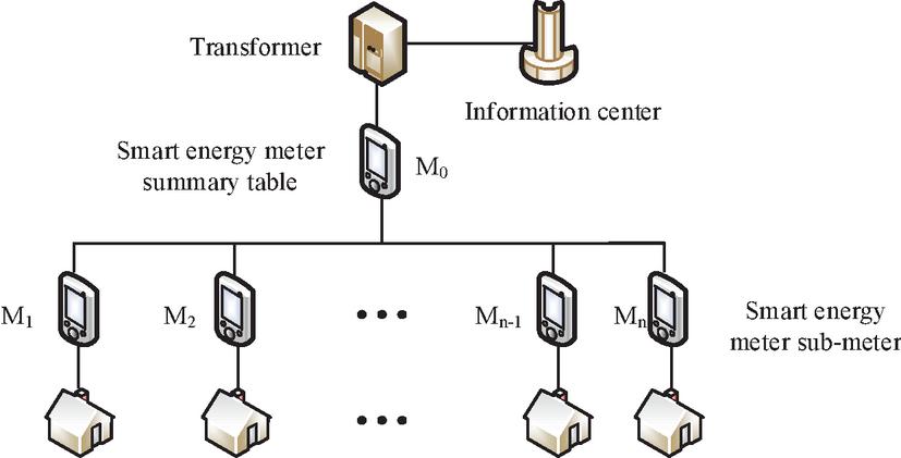
Figure 1 Topology diagram of smart energy meter.

The current household smart energy meter is a one-way electricity meter with a rated voltage of 220 V, installed in the low-voltage power grid. In addition to smart meters in this power grid, devices such as concentrators and data collectors are also installed to perform data collection and transmission. The structure of the power grid data collection is shown in Figure 2. Transformers convert high-voltage supply from the power grid into low-voltage power supply, with concentrators installed at their output terminals. The concentrator can be directly connected to the electricity meter or to the collector, and then connected to the electricity meter. The concentrator sends commands to the electricity meter to collect data from the electricity meter. The data collection of electricity meters can be divided into two types: real-time collection and timed collection. Real-time collection refers to the data collection command issued by the concentrator to the electricity meter. After receiving the command, the electricity meter sends the data to the concentrator, which transmits the data to the data center of the system. Timed collection first sets the collection time of the electricity meter, then regularly sends the data of the electricity meter to the concentrator, and finally transmits it to the data center. In low-voltage power systems, various communication methods are used, including RS-485 communication, wireless network communication, carrier communication, infrared communication, fiber optic communication, power frequency meter reading, general packet radio service meter reading, etc. In close proximity, communication in energy meters and concentrators, collectors and concentrators are usually achieved through RS485 or power line carriers. Since the distance between concentrators and data centers is usually large communication is usually achieved through fiber optic or wireless means.

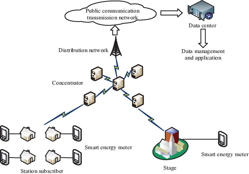
Figure 2 Structure of power grid data acquisition system.

The data required for online error estimation of smart energy meters is divided into two main parts: the metering data of the energy meter and the information data of the system [17]. If abnormal data occurs at time $\eta$, the detector must quickly detect and reduce the error rate in the shortest possible time to achieve the minimum anomaly detection delay and false alarm rate. When the system operates normally, it will not cause any loss to the system. However, if the system operates abnormally, it will incur losses. If $r_t$ is defined as the loss after the detector performs an action $a_t$ in state $s_t$, Equation (1) can be obtained.

$$r_t=\{\begin{array}{c}0,(s_t=s_n,a_t=a_c)\hfill \\ c_1,(s_t=s_n,a_t=a_s)\hfill \\ 0,(s_t=s_a,a_t=a_a)\hfill \\ c_2,(s_t=s_a,a_t=a_c)\hfill \end{array}$$

(1)

When the data in the environment is in a normal state, the detector chooses to continue analyzing. When the data is in an abnormal state, the detector chooses to stop analyzing. In these two situations, the detector performs the correct operation. At this time, the detector has no loss, and $r=0$. Under normal circumstances, the detector stops analyzing, resulting in incorrect behavior and causing system loss of $c_1$. If the data is in an abnormal state but the detector decides to continue analysis, the system loss is $c_2$.

The basic idea of Q-learning is for intelligent agents to interact with the environment, perceive the environment state, and achieve maximum returns in interacting with the environment. The interaction between intelligent agents and the environment is represented by Markov Decision Process (MDP). $r$ is the loss after the detector takes action. The objective of MDP is $\min E|{\sum }_{t=0}^{\mathrm{\infty }}{\gamma }^t{r}_t|$ to minimize the total loss of the detector. The time when the detector takes the termination action is $T_s$, the discount coefficient is $\gamma =1$, and the data is abnormal at time $\eta$. The expected value of the loss is expressed as Equation (2).

$$E\left|\sum _{t=0}^{\mathrm{\infty }}{\gamma }^t{r}_t\right|=c_1{P}_{\eta }(T_s<\eta )+c_2{E}_{\eta }|{(T_s<\eta )}^{\prime }|$$

(2)

In Equation (2), $P_{\eta }$ represents the probability of data anomalies occurring at time $\eta$. The value of ${(T_s<\eta )}^{\prime }$ is $((T_s<\eta ),0)$. The final anomaly data detection model can be expressed as Equation (3).

$$\min c_1{P}_{\eta }(T_s<\eta )+c_2{E}_{\eta }|{(T_s<\eta )}^{\prime }|$$

(3)

After adjusting $c_1$ and $c_2$, a balance can be achieved between detection delay and error detection. Generally, when the ratio $c_1/c_2$ is greater than 1, the error detection rate can be reduced. When the environmental data contains abnormal data, and $s_t=s_a$. If the detector erroneously chooses to continue detecting action $a_t=a_c$, the loss is defined as Equation (4).

$$r_t=\{\begin{array}{c}0,(s_t=s_a,a_t=a_c)\hfill \\ c_2^{\prime }|t-\eta |,(s_t=s_a,a_t=a_s)\hfill \end{array}$$

(4)

When the environmental data is normal, $s_t=s_n$. If the detector erroneously chooses to continue detecting the action, and $a_t=a_s$, the loss is represented by Equation (5).

$$r_t=\{\begin{array}{c}0,(s_t=s_n,a_t=a_c)\hfill \\ c_1^{\prime }|t-\eta |,(s_t=s_n,a_t=a_s)\hfill \end{array}$$

(5)

2.2 Analysis of Line Energy Loss Based on DBN

Line loss seriously affects the accuracy of an energy meter error estimation. It is necessary to accurately evaluate the line loss and remove it from the total meter energy measurement value when solving the energy meter error matrix equation [18]. In the case of various types and features of abnormal power data, the Q-learning method has difficulty to effectively learn this type of data, leading to a decrease in detection accuracy [19]. When there are many types of abnormal data and the environmental factors involved are complex, the algorithm is prone to divergence during the learning process, resulting in slow convergence and a decrease in algorithm performance. Therefore, a new method for detecting abnormal data in electricity meters based on HDQL is proposed to judge the abnormal data. The framework structure is shown in Figure 3.

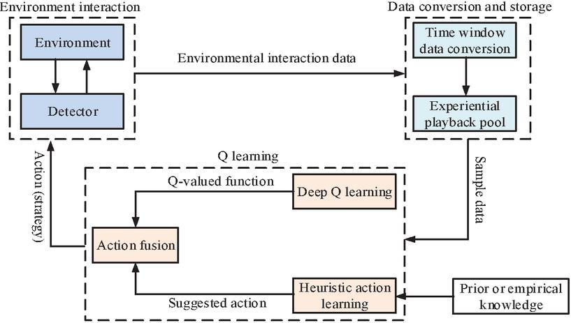
Figure 3 HDQL frame structure schematic.

A heuristic behavior learning model is introduced in the Q-learning model to effectively guide Q-learning. To ensure the global stability and convergence, it is fused with the optimal decision behavior output by the deep Q-learning model to guide the decision-making behavior of the detector.

Heuristic action learning can integrate both prior knowledge and experiential knowledge [20]. When there is a strong correlation between the measurement data of two observation periods, it is observed that if the data of one period is normal, the data of the other period is also likely to be normal. Therefore, the correlation between the data can be used to generate heuristic behavior learning recommendation behavior. The correlation between data can be expressed by the Pearson correlation coefficient. The correlation coefficient between the sub-meter energy data during the $i$-th measurement cycle and the $i-1$-th period is expressed as Equation (6).

$${\rho }_{i,i-1}=\frac{{\sum }_{k=1}^{m_s}(({\psi }_k(i)-{\overline{\psi }}_k(i))({\psi }_k(i-1)-{\overline{\psi }}_k(i-1)))}{\sqrt{{\sum }_{k=1}^{m_s}{({\psi }_k(i)-{\overline{\psi }}_k(i))}^2}\sqrt{{\sum }_{k=1}^{m_s}{({\psi }_k(i-1)-{\overline{\psi }}_k(i-1))}^2}}$$

(6)

In Equation (6), ${\psi }_k(i)$ represents the electricity metering value of the $k$-th sub-meter during the $i$-th period. ${\overline{\psi }}_k(i)$ signifies the average value of all sub-meter electricity metering values during the $i$-th period. ${\psi }_k(i-1)$ signifies the electricity metering value of the $k$-th sub-meter in the $i-1$-th period. ${\overline{\psi }}_k(i-1)$ signifies the average value of all sub-meter electricity metering values during the $i-1$-th period. The correlation coefficient ${\rho }_i$ of the $i$-th measurement period data is the average of the $i$-th measurement period data and the adjacent $N_L$-th period data, expressed as Equation (7).

$${\rho }_i=\frac{1}{N_L}\sum _{k=1}^{N_L}{\rho }_{i,i-k}$$

(7)

The data in the $N_L$ period adjacent to the $i$-th measurement period are all normal values. Otherwise, the model stops learning and deletes abnormal data. Therefore, if the correlation is high, the data being normal is higher. The suggestive learning suggestion action ${\pi }_A(s)$ generated by data correlation is expressed as Equation (8).

$${\pi }_A(s)=\{\begin{array}{cc}{a}_c,\hfill & \mathit{if}{\rho }_i\ge {\rho }_H\hfill \\ a_s,\hfill & \mathit{if}{\rho }_i<{\rho }_H\hfill \end{array}$$

(8)

In Equation (8), ${\rho }_H$ represents the correlation coefficient threshold. By adjusting the correlation coefficient threshold ${\rho }_H$, the sensitivity of the heuristic behavior learning model to identifying abnormal data can be adjusted. The recommendation behavior is fused with the behavior corresponding to the optimal Q-value function output by the deep Q-learning model in the form of probability, which can be expressed as Equation (9) in the scene $i$.

$$\pi (s)=\{\begin{array}{c}{\pi }_A(s),ran{d}_i\le {\chi }_i\hfill \\ {\pi }_Q(s),ran{d}_i>{\chi }_i\hfill \end{array}$$

(9)

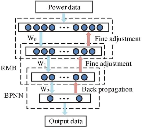
Figure 4 Schematic diagram of DBN line loss analysis mode.

In Equation (9), $\pi (s)$ represents the final strategy action output by Q-learning. ${\mathit{rand}}_i$ represents a random number that follows a uniform distribution on the [0,1] interval. ${\chi }_i$ represents the fusion probability corresponding to the measurement period data on the $i$ side. ${\pi }_Q(s)$ is the strategy action output by the depth Q-learning. When ${\mathit{rand}}_i$ is lower than the fusion probability, the strategy proposed by a heuristic behavior learning model is output. On the contrary, a decision strategy based on deep Q-learning is used. As the detector learns for a period of time and becomes fully familiar with the environmental features, it can reduce the recommended operations. Therefore, the fusion probability is shown in Equation (10).

$${\chi }_i=\{\begin{array}{cc}0,\hfill & i<t_L\hfill \\ \chi ,\hfill & t_L\le i<t_U\hfill \\ 0.99{\chi }_{i-1},\hfill & t_U<i\hfill \end{array}$$

(10)

In Equation (10), $t_L$ represents the number of scenes where the suggested strategy is started. $\chi$ represents the set fusion rate. $t_U$ represents the number of scenes when the fusion probability begins to decrease. Deep Belief Network (DBN) is a probabilistic generative method that uses multiple Restricted Boltzmann Machines (RBMs) to effectively extract features from data. Figure 4 shows the DBN line loss analysis mode.

The RBM hidden layer in DBN plays a role in feature mining. As the number of layers increases, it can better mine the data information, but it also greatly affects the training speed and execution efficiency of the network. In this model, the network structure of RBM adopts a three-layer structure. In the network, the input layer nodes are related to the sub-tables in the network. The hidden layer nodes in the middle can be set according to an empirical equation, as shown in Equation (11).

$$n_{\mathit{node}}=\lfloor \sqrt{n_{\mathit{input}}+n_{\mathit{output}}}+n_{\mathit{noderandom}}\rfloor$$

(11)

In Equation (11), $n_{\mathit{node}}$ represents the number of hidden layer nodes. $n_{\mathit{input}}$ represents the input feature dimension of the hidden layer. $n_{\mathit{output}}$ signifies the output feature dimension. $n_{\mathit{noderandom}}$ represents a random integer within the interval [1, 10]. If each sampled data contains positive active power and electricity data, and there are no outliers in the line energy data, the energy consumption $e_{\mathit{loss}}(i)$ of the line can be calculated, as shown in Equation (12).

$$e_{\mathit{loss}}(i)=N_L{K}^2{I}_{pj}{(i)}^2{R}_{dz}(i)t(i)\times {10}^{-3}$$

(12)

In Equation (12), $K$ represents the shape coefficient of the load curve. $I_{pj}$ represents the equivalent resistance of the lines in the circuit. $R_{dz}$ represents the average value of the load current. $R_{dz}$ is displayed in Equation (13).

$$R_{dz}(i)=\frac{1}{N_{L,j}}\sum _{j=1}^{m_s}{I}_{zdok,j}^2(i)R_j{N}_L{I}_{zd}^2(i)$$

(13)

In Equation (13), $N_{L,j}$ represents the structural coefficient of the low-voltage power grid. $I_{\mathit{zdok},j}$ represents the maximum current in the $j$-th branch. $R_j$ represents the resistance in the $j$-th branch. $I_{\mathit{zd}}$ represents the maximum current of the main circuit. The total table data ${\psi }_0{(i)}_{\mathit{generate}}$ is displayed in Equation (14).

$${\psi }_0{(i)}_{\mathit{generate}}=\sum _{j=1}^{m_s}\frac{{\psi }_j(i)}{1+{\sigma }_j}+e_{\mathit{loss}}(i)+\epsilon (i)$$

(14)

In Equation (14), ${\sigma }_j$ signifies the error value of the $j$-th sub-table. ${\psi }_j(i)$ represents the electricity metering value of the $j$-th sub-meter in the $i$-th measurement period data. $\epsilon (i)$ represents the small error in the system during the $i$-th measurement period. The line loss rate is expressed as Equation (15).

$$\xi (i)=\frac{e_{\mathit{loss}}(i)}{{\psi }_0{(i)}_{\mathit{generate}}}$$

(15)

3 Verification of Measurement Accuracy of Smart Energy Meters

A 20,000-scene dataset is generated based on 1,032 days of electricity metering data. The number of sub-tables in the system is 100, and the duration of each scene is 200. The data is divided into two equal parts and set to generate abnormal data at different time points to analyze the algorithm’s discriminative performance against abnormal data. The study divides abnormal data into three categories: continuous small deviation, continuous large deviation, and mixed. Accuracy, precision, recall, and Area under Receiver Operating Characteristic (ROC) Curve (AUC) are selected as the four indicators to evaluate the model. False Positive Rate (FPR) refers to the proportion of samples that are incorrectly predicted as positive among all samples that are actually negative.

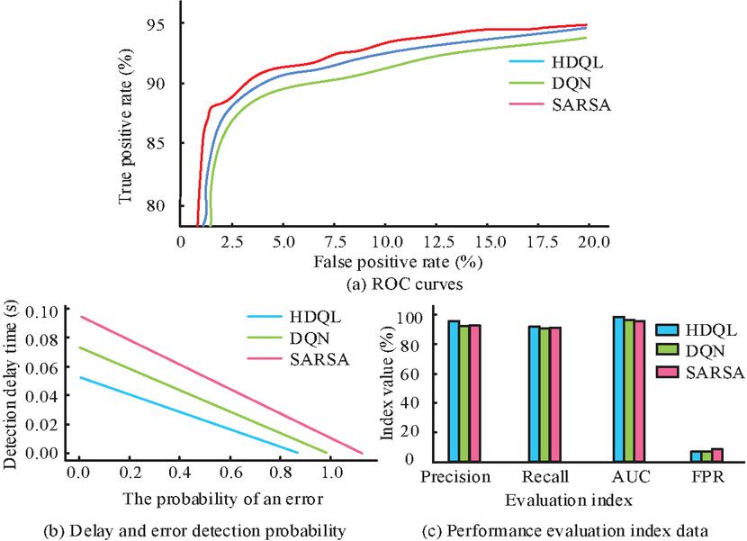
Figure 5 Detection results of continuous small deviation abnormal data.

3.1 Abnormal Data Analysis

The HDQL, State-Action-Reward-State-Action (SARSA), and Deep Q-Network (DQN) are used for detecting continuous small deviation outliers. The testing results are shown in Figure 5. From Figures 5(a) and 5(c), the AUC of the HDQL was 96.35%, which reduced its ability to detect continuous small deviations. The AUC decreased to 94.25%. The AUC detected by the HDQL was the largest among the three methods. From Figure 5(b), the probability of errors occurring in the HDQL algorithm was 0.56, which was much higher than that of the discretization. The errors of the other two methods were 0.69 and 0.95, respectively. In terms of detection speed, the average latency of HDQL was 0.86 seconds, which was faster than DQN (0.97 seconds) and SARSA (1.13 seconds), making it suitable for real-time monitoring scenarios where early detection of subtle anomalies is critical.

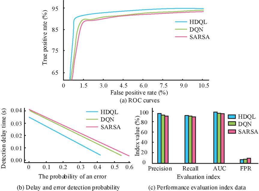
Figure 6 Detection results of continuous large deviation abnormal data.

The detection results of continuous large deviation abnormal data are shown in Figure 6. From Figures 6(a) and 6(c), the AUC of HDQL was 98.77%, DQN was 98.16%, and SARSA was 97.89%, indicating that the HDQL algorithm was the most accurate. The AUC of continuous large deviation data is larger than that of continuous small deviation data, indicating that it can more accurately detect large deviation abnormal data. From Figure 6(b), the HDQL had a data error rate of 3.52% in a single time period, which was the smallest among the three methods, and the delay rate was also the smallest. Compared with analyzing continuous small deviation data, the HDQL had a lower error rate and delay when analyzing continuous large deviation data. From Figure 6(c), the accuracy of HDQL for continuous large-deviation anomalies reached 96.13%, which was superior to that of DQN (92.58%) and SARSA (90.21%). This improvement can be attributed to the ability of the heuristic module to utilize the prior knowledge of abnormal data continuity, reducing the true positive rate by 18% compared with DQN. It is worth noting that the FPR of HDQL was 4.13%, which was 6.7% lower than that of SARSA, demonstrating its robustness to noise in high-bias scenarios.

The HDQL algorithm is compared with SVM, Decision Tree (DT), Back Propagation Neural Network (BPNN), Linear Regression (LR), Adaboost, KNN, and Bayes. From Figure 7, HDQL had the highest AUC in mixed anomaly detection, reaching 98.95%, which exceeded that of traditional algorithms such as BPNN (95.63%), SVM (94.87%), and Adaboost (94.32%). This performance improvement is attributed to the dual-architecture of the algorithm. The deep Q-learning module captures the complex nonlinear relationships in the mixed anomalies, while the heuristic module filters out the normal fluctuations through the correlation coefficient threshold. For example, when dealing with exceptions combining large and small deviations, the accuracy of HDQL reached 96.13%, which was significantly higher than that of the comparison methods. This algorithm has the ability to dynamically weight heuristic recommendations and deep learning outputs, ensuring robustness in different types of abnormal situations.

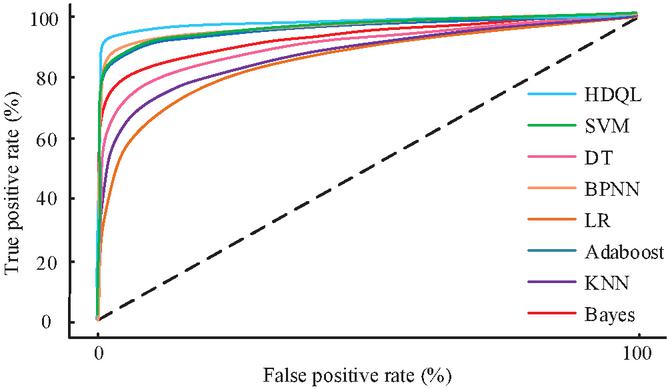
Figure 7 ROC curve of various algorithms in mixed abnormal data detection.

3.2 Line Loss Estimation

Table 1 compares the calculation errors of line losses for different models, including Root Mean Square Error (RMSE), Mean Absolute Error (MAE), and Mean Absolute Percentage Error (MAPE). According to Table 1, the Adaboost method had the largest MAE, while the proposed HDQL model had the smallest value. HDQL model could better track the line loss changes and make accurate predictions when line loss suddenly changed. For MAPE, the Adaboost and SVR models had larger values, while the HDQL model value was the smallest, demonstrating the excellent analysis and estimation ability for line losses.

Table 1 Comparison of line loss calculation errors

Model	RMSE	MAE	MAPE
Random forest	0.25%	0.26%	4.63%
Gradient boosting	0.27%	0.26%	4.32%
Adaboost	0.29%	0.29%	6.42%
Extra trees	0.26%	0.25%	4.96%
SVR	0.21%	0.24%	7.86%
RBF network	0.22%	0.25%	2.34%
HDQL	0.19%	0.15%	1.86%

Figure 8 shows the accuracy of the HDQL algorithm in different line loss scenarios when the number of sub-tables is 20, 40, 60, 80, and 100. From Figure 8, when the line loss was large, the accuracy of error estimation decreased with the increase of line loss. When the online loss was less than 7.43%, the accuracy was above 90%. When the number of sub-tables was small, there was a significant fluctuation in accuracy. When there were many sub-tables, the accuracy decreased as the number of sub-tables increased. When the number of sub-meters exceeded 40 and the maximum line loss reached 10%, the accuracy reached 80%–85%.

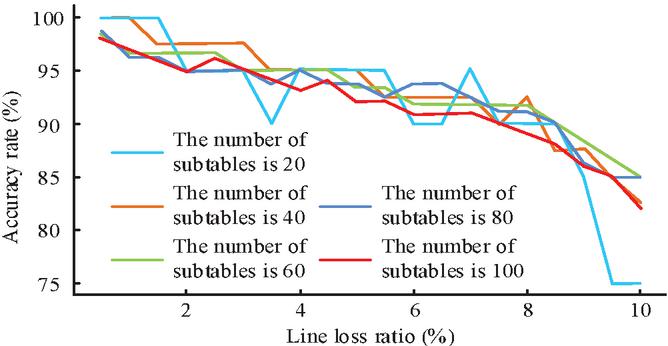
Figure 8 Accuracy of HDQL algorithm after application under different line loss rate and number of sub-tables.

3.3 Case Validation

The experimental data is sourced from the power company, which is the electricity metering data for a certain substation area. The data time range is from May 18, 2020 to April 22, 2023. One total meter and 61 sub-meters are installed in the substation area. The collected electricity meter data is frozen data at 24:00 hrs. every night, and the data collection frequency is one day. Table 2 shows a data example from five electricity meters during the same time period.

Table 2 Data sample

Date of measurement	2023.01.15
Energy meter identification	319545263	319652481	319652469	319652485	319524123
Rated current	Basic current: 5A, Maximum current: 60A
Composite ratio	1	1	1	1	1
Metering point characteristic	0	0	0	0	0
CT variable ratio	1	1	1	1	1
PT variable ratio	1	1	1	1	1
Whether the photovoltaic equipment is running	No	No	No	No	No
Positive active total	8,846.32	12,145.63	5,596.36	6,254.10	6,268.36

The test set data is fed into the trained HDQL, and suspicious abnormal data is detected. The analysis results are shown in Figure 9. The abnormal determination condition is that the action output is stopped $a_s$ and the correlation coefficient is ${\rho }_i<{\rho }_H$. During the initial 30 days of observation, 10 out of the total data points were identified as abnormal, primarily due to significant load fluctuations caused by new user connections and equipment debugging in the substation area. As the model trained on more data, the heuristic fusion probability gradually adjusted, reducing false positives for normal seasonal load changes. By the 471st day, there were only 4 abnormal datasets left, all of which corresponded to sudden load surges exceeding 150% of the rated capacity. This demonstrates that HDQL model can adapt to the steady-state operation of the power grid over time while maintaining sensitivity to transient anomalies.

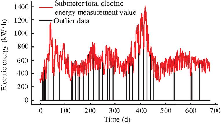
Figure 9 Abnormal data detection results.

Figure 10 shows the error estimation at different system loss rates. Figures 10(a) and 10(b) show the RMSE and MAE of error estimation at different comprehensive loss rates, respectively. The error gradually increased with the increase of the comprehensive loss rate. When the total loss rate does not exceed 8%, comparisons are made using HDQL and DBN methods. From the results, the RMSE and MAE of error estimation gradually increased with the increase of the total loss rate. When the combined loss rate was 10%, the growth rate of RMSE and MAE significantly accelerated. Without HDQL and DBN algorithms, the maximum RMSE was 1.27% and the maximum MAE was 1.28%. After using HDQL and DBN algorithms, the maximum RMSE was 0.68% and the maximum MAE was 0.67%, which decreased by 46.46% and 47.66%, respectively, significantly reducing the error estimation bias. The above results indicate that the heuristic module of HDQL is more sensitive to continuous small-deviation anomalies by capturing the temporal correlation of data, while traditional DQN is prone to ignore low-amplitude anomalies due to its dependence on pure data-driven methods.

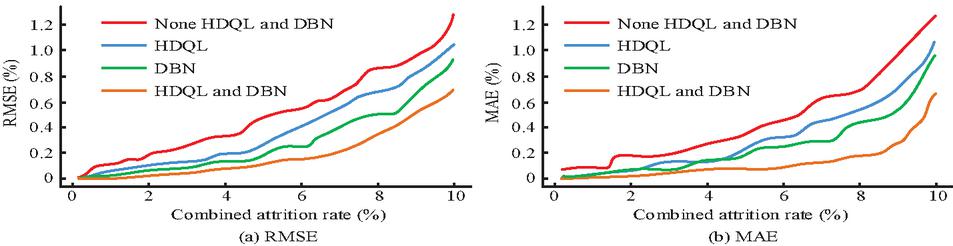
Figure 10 Online error estimation of smart energy meters.

4 Conclusion

In response to the poor real-time and low accuracy of error estimation in the current online measurement process of electric energy meters, as well as the impact of abnormal measurement data and line energy loss on the electric energy meter error estimation, this article designed an environment interaction method and a state mapping method based on MDP. The deep Q-learning detection algorithm introduced with heuristic learning module was used to identify data features and abnormal data of electric meters. The relationship between electricity metering values and line energy losses was analyzed from multiple dimensions to reduce the impact of line losses on online error estimation. The results showed that the AUC values of the HDQL algorithm in analyzing continuous small deviation, continuous large deviation, and mixed anomaly data were 96.35%, 98.77%, and 98.75%, respectively. When the anomaly coefficient was less than 0.084 and the number of sub-tables did not exceed 100, the accuracy of the online error estimation algorithm was higher than 90%, and the accuracy was significantly improved. When the line loss rate was less than 7.5% and the number of sub-meters did not exceed 100, the accuracy of the online error estimation algorithm was higher than 90%, greatly reducing the interference of line energy loss on the online error estimation. However, the model relies on the topological and load characteristics of specific transformer areas. Meanwhile, due to the differences in line loss patterns and anomaly types among different transformer areas (such as different load fluctuations between industrial transformer areas and residential transformer areas), retraining is required when directly migrating to a new area. In the future, it is planned to introduce transfer learning technology to enhance the generalization ability of the model through cross-regional data sharing, or develop an adaptive parameter adjustment mechanism to dynamically adapt to different power grid environments.

References

[1] Usman A M, Abdullah M K., “An assessment of building energy consumption characteristics using analytical energy and carbon footprint assessment model”. Green and Low-Carbon Economy, 2023, 1(1): 28–40.

[2] Aryavalli S N G, Kumar G H., “Futuristic vigilance: Empowering chipko movement with cyber-savvy IoT to safeguard forests”. Archives of Advanced Engineering Science, 2023, 1(8): 1–16.

[3] Bae J, Lee J, Chong S., “Learning to schedule network resources throughput and delay optimally using Q-learning”. IEEE/ACM Transactions on Networking, 2021, 102(99): 1–14.

[4] Liu K, Sun Y, Yang D., “The administrative center or economic center: Which dominates the regional green development pattern. A case study of Shandong Peninsula urban agglomeration, China”. Green and Low-Carbon Economy, 2023, 1(3): 110–120.

[5] Badr M M, Ibrahem M I, Mahmoud M, Fouda M M, Alsolami F, Alasmary W., “Detection of false-reading attacks in smart grid net-metering system”. IEEE Internet of Things Journal, 2022, 9(2): 1386–1401.

[6] Wang D, Zhang W, He H, Yu C T., “Efficient hybrid central processing unit/input-output resource scheduling for virtual machines”. IEEE Transactions on Industrial Electronics, 2021, 68(3): 2714–2724.

[7] Wang Y, Liu Y T, Chen W, Ma Z M, Liu T Y., “Target transfer Q-learning and its convergence analysis”. Neurocomputing, 2020, 392(7): 11–22.

[8] Xiang B I, Huang H, Zhang B, Xing W., “A hybrid routing algorithm for V2V communication in VANETs based on blocked Q-learning”. IEICE Transactions on Communications, 2022, 8(1): 1–73.

[9] Ilker G, Ozsoydan F B., “Q-learning and hyper-heuristic based algorithm recommendation for changing environments”. Engineering Applications of Artificial Intelligence, 2021, 102(4): 1084–1103.

[10] Lim S, Yu H, Lee H., “Optimal tethered-UAV deployment in A2G communication networks: Multi-agent Q-learning approach”. IEEE Internet of Things Journal, 2022, 9(19): 18539–18549.

[11] Fekri M N, Patel H, Grolinger K, Sharma V., “Deep learning for load forecasting with smart meter data: Online adaptive recurrent neural network”. Applied Energy, 2020, 282(3): 116177.1–116177.17.

[12] Yan S, Li K, Wang F, Yan S, Wang F., “Time-frequency features combination-based household characteristics identification approach using smart meter data”. IEEE Transactions on Industry Applications, 2020, 56(3): 2251–2262.

[13] Biswas S, Himanshu G S, Das P, Saha K, De S., “Efficient data transfer mechanism for DLMS/COSEM enabled smart energy metering platform”. Performance Evaluation Review, 2023, 50(4): 14–16.

[14] Zakariazadeh A., “Smart meter data classification using optimized random forest algorithm”. ISA Transactions, 2021, 126(3): 361–369.

[15] Qaisar S M, Alsharif F., “Event-driven system for proficient load recognition by interpreting the smart meter data”. Procedia Computer Science, 2020, 168(26): 210–216.

[16] Cao H, Wu Y, Bao Y, Feng X, Wan S, Qian C., “UTrans-Net: A model for short-term precipitation prediction”. Artificial Intelligence and Applications, 2023, 1(2): 106–113.

[17] Zhao B, Ye M, Stankovic L, Stankovic V., “Non-intrusive load disaggregation solutions for very low-rate smart meter data”. Applied Energy, 2020, 268(14): 949–962.

[18] Wang J, Srikantha P., “Stealthy black-box attacks on deep learning non-intrusive load monitoring models”. IEEE Transactions on Smart Grid, 2021, 12(4): 3479–3492.

[19] Ly A, El-Sayegh Z., “Tire wear and pollutants: An overview of research”. Archives of Advanced Engineering Science, 2023, 1(1): 2–10.

[20] Garai S, Paul R K, Kumar M., “Intra-annual national statistical accounts based on machine learning algorithm”. Journal of Data Science and Intelligent Systems, 2023, 2(2): 12–15.

Biographies

Fanqin Zeng graduated from South China University of Technology with a Master’s degree in Control Science and Engineering (2020). Currently, he is working as a specialist in the Energy Data Department of the Measurement Center of Guangdong Power Grid Co., Ltd. His areas of interest include machine learning, image processing, and data analysis.

Xiling Tang graduated from Xi’an Jiaotong University, majoring in Instrumentation and Measurement. At present, he has published articles in multiple professional journals and core centers, and his areas of expertise include intelligent terminals, load management, and measurement related majors.

Yingxiong Leng, born in November 1995 in Jiujiang, Jiangxi, obtained a master’s degree in Computer Technology from Dalian University of Technology in 2021. Engineer who has published articles in various professional journals and EI conferences, with a main research focus on the application of artificial intelligence in power systems.

Hengxiang Yu graduated from Northeast Electric Power University, majoring in Electrical Engineering and Automation. Currently, I am a senior economist and expert in customer problem management, and have published articles in various professional journals and Chinese language journals. His areas of interest include full process control of customer demands, intelligent customer service, business expansion, and large-scale model applications.

Distributed Generation & Alternative Energy Journal, Vol. 40_4, 845–868.
doi: 10.13052/dgaej2156-3306.40410
© 2025 River Publishers