Early Detection of Sulfur Hexafluoride Leakage in Substation Based on Numerical Simulation and Finite Volume Method

Minglei Wei

State Grid Hebei Electric Power CO. LTD., Shijiazhuang, 050000, China
E-mail: mingleiwm@outlook.com

Received 19 June 2025; Accepted 01 September 2025

Abstract

Sulfur hexafluoride (SF6) is an excellent insulating gas that is widely used in substations. However, it poses a threat to worker safety in the event of a leakage. Therefore, it is crucial to construct an accurate early-warning detection system for leaks to ensure the safe operation of substations. In this study, taking a substation as an example, the key parameters affecting SF6 gas diffusion were analyzed by novel numerical simulation model. On this basis, combined with the finite volume method, different leakage scenarios are simulated. Under different leakage conditions, SF6 could accumulate significantly on the ground. Its volume concentration could exceed 1000 ppm, and the duration of the high concentration state could be longer than in the horizontal leakage scenario. The method proposed in this study can effectively reduce the impact of leakage accidents, and provide a theoretical basis for the early monitoring and detection of SF6 leakage.

Keywords: Numerical simulation, substation, sulfur hexafluoride, concentration, leak diameter.

1 Introduction

Sulfur hexafluoride (SF6) is a new generation ultra-high-voltage insulating dielectric material, and is widely used in substations because of its good gas insulation properties. However, when SF6 gas leaks, it reacts with water vapor to form acidic substances. It can pose potential hazards to the human respiratory system and accelerate the corrosion and aging of metal components and insulating materials within substations. This leads to a decline in equipment insulation performance, shortened operational life, and even power grid failures and shutdowns. Although the likelihood of SF6 leakage accidents in substations is relatively low, these accidents often pose a significant threat to personnel health and equipment maintenance costs, endangering the safe and stable operation of the power system. Therefore, establishing an accurate and efficient SF6 leakage early-warning detection mechanism is highly valuable from an engineering standpoint, as it reduces the impact range of leakage accidents and minimizes economic losses. The current methods to study the gas leakage diffusion process include diffusion modeling, detection experiments, and numerical simulation (NS) [1–3]. NS has become the main way to study gas diffusion because of its advantages such as low cost and short time consuming [4]. In view of this, this study proposes an SF6 leakage early warning model based on NS that combines the discretization scheme of the finite volume method with the diffusion characteristics of SF6 heavy gas and the patented technology in reference [5]. This model forms a complete early warning detection system.

The innovative combination of NS and the finite volume method is this study’s main contribution. This approach effectively handles complex boundary conditions and nonlinear problems, improving the accuracy and reliability of SF6 diffusion simulations. The study examines how the diameter of the leakage port and the leakage location affected the gas diffusion. This analysis reveals the accumulation and diffusion characteristics of SF6 in the substation. This knowledge provides a quantitative basis for the early detection of leakage.

This study is organized in four sections. The first section presents the relevant research achievements of scholars at home and abroad in the fields of NS and gas diffusion, and analyzes the deficiencies of the existing research. The second section mainly elaborates on the construction process of the proposed SF6 leakage early detection model. The third section mainly analyzes the diffusion law and monitoring data of SF6 gas under different parameters. The fourth section is the summary of this study, points out the shortcomings of the proposed model, and puts forward the future research directions.

2 Related Works

Many scholars have used NS in many fields [6–8]. El Jery A et al. applied the NS method to the subcooled boiling problem of sub-oxygen nanofluids. The study employed the Eulerian-Lagrangian approach to simulate the interaction between the base fluid and the nanoparticles, as well as the Eulerian method to simulate the contraction response between the base fluid and the vapor. The two procedures produced different results, but the differences between the two ways grew as the particle concentration rose. When the volume fraction of nanoparticles rose from 0.28% to 0.561%, the average volume fraction difference increased from 16.13% to 28.3% [9]. Maranzoni et al. used the NS approach in the two-dimensional steep slope shallow water equation (SSSWE) to generate a new formulation of the SSSWE model. The findings showed that, on a frictionless river, the newly obtained SSSWE model formulation is slower than the traditional shallow water equation (SWE). In experimental tests, the equation was found to be practical [10]. Park S et al. developed a numerical model in a bubble tower reactor in combination with a molten catalyst. The study considered continuous as well as discrete bubbles on the basis of non-isothermal one-dimensional simplification and initial bubble properties were predicted by correlation. Finally, through sensitivity analysis, the results showed that the catalyst density can effectively affect the methane conversion under pressure [11]. Jüngel et al. suggested an implicit Eulerian finite volume scheme constructed on a general cross-diffusion system with volume filling restrictions. The diffusion matrix was not positive semidefinite and its formal gradient flow structure was assumed. The numerical scheme proposed in the study had a continuous inequality with a discrete entropy structure in it. Experimental results indicated that the scheme was convergent and could be realized in two-dimensional thin-film solar cell systems [12].

Many scholars have studied the gas leakage problem. Li et al. conducted a numerical analysis of a mobile hydrogen refueling station’s hydrogen leakage issue. The study examined the size of the hydrogen cloud and how hydrogen was distributed. It also examined the impact of two parameters – leak location and leak flow rate – on hydrogen diffusion. The findings showed that when the leak location varied, so did the hydrogen concentration. At different locations, the hydrogen concentration reached 0.4% and 4%, respectively. The volume growth of hydrogen was exponential in the unenclosed space [13]. Petersen H I et al. proposed a method of combining mud with seismic data in the study of leakage phenomena. Gas data from mud could provide detailed information about the gas in the overburden. The gas with higher carbon number could indicate the migration of heat-producing gas. If the heat-producing gas had migrated significantly, it would indicate a reduction in seal integrity. If there was no significant migration of heat-producing gases, the seal had integrity. The results showed that this method could provide technical support for localized seal integrity assessment [14]. To solve the problem of existing algorithms’ inability to adaptively enhance SF6 leakage areas or suppress Gaussian noise, researchers like Quan proposed an SF6 leakage area enhancement algorithm based on improved histogram equalization. First, the algorithm used a single-scale retina to process the original SF6 image and obtain a reflected image. Then, it used guided filtering to decompose the reflected image into a detail layer and a base layer. Finally, it used improved histogram equalization to adaptively process the base layer and fused the enhanced images to obtain the final image. The results demonstrated that the algorithm could adaptively enhance the contrast of the leakage area and effectively preserve edges while suppressing Gaussian noise [15]. In order to effectively manage and maintain SF6 power equipment, Zhang et al. proposed a dynamic prediction model for SF6 weight based on the non-ideal gas state equation and the improved random forest algorithm. The model used gas pressure and temperature sensors to measure the SF6 gas pressure and temperature dynamically. It then used the non-ideal gas state calculation equation to convert these values into the weight of the SF6 gas. The model was established by combining the improved chimpanzee optimization algorithm and the random forest algorithm. The results showed that the average absolute error, root mean square error, and mean absolute percentage error of this method were 51.54 kg, 103.59 kg, and 11.62%, respectively [16].

In conclusion, while many scholars have conducted in-depth research on SF6 gas leakage, most studies have focused on idealized scenarios. These studies lack precise modeling of substation internal environments, which makes it difficult to accurately simulate SF6 gas diffusion laws after leakage. Therefore, the research creatively combines NS and finite volume method applied in SF6 early warning to realize effective monitoring and early warning of SF6. The study will provide theoretical support for the emergency management of SF6 leakage accidents, and provide reference for the design of substation rooms and evacuation of personnel. Compared to existing methods, this method uses NS to efficiently handle complex boundary conditions and nonlinear problems, providing an accurate physical model for gas diffusion. It uses the finite volume method to efficiently and stably handle large-scale complex flow fields. This combination compensates for the limitations of traditional methods in complex scenarios, significantly improving the simulation’s accuracy and reliability.

3 Construction of SF6 Leakage Early Warning Model for Substation

To perform the selection and calculation of SF6 leakage early warning models, the NS model needs to be analyzed first. Then, it is combined with the finite volume method to build a physical model.

3.1 Numerical Simulation Computational Modeling

The analysis is carried out in the setting of an underground substation where SF6 gas can leak and spread outside due to a leaking opening in the valve on the pipe that connects the transformer to the heat exchanger in the main substation room. The transformer has a high pressure, and the SF6 gas in the piping continues to leak until the ambient pressure equals the transformer pressure. The pressure differential between the inside and outside of the pipeline causes SF6 gas to spread quickly when a leaky opening occurs in the valve on the connecting pipeline. The SF6 leakage mass flow rate (LMFR) is calculated by gas leakage mass modeling. Whether or not the SF6 gas at the leakage port is flowing at the speed of sound affects the choice of model, and is usually judged using the critical pressure ratio (CPR). CPR is expressed as shown in Equation (1).

$$\mathit{CPR}={\left(\frac{2}{K+1}\right)}^{\frac{K}{K-1}}$$

(1)

In Equation (1), $\mathit{CPR}$ represents the critical pressure ratio. $K$ represents the specific heat capacity. If $\frac{P_0}{P}\le \mathit{CPR}$, SF6 gas flows at the speed of sound. $P_0$ represents the working pressure of the transformer. $P$ represents the ambient pressure. All in units of Pa. Meanwhile, the LMFR of the gas is calculated according to Equation (2).

$$Q=C_0{A}_{0}P{\left[\frac{\mathit{MK}}{\mathit{ZRT}}{\left(\frac{2}{K+1}\right)}^{\frac{K}{K-1}}\right]}^{\frac{1}{2}}$$

(2)

In Equation (2), $Q$ is the LMFR in kg/s. $C_0$ is the leakage coefficient and $A_0$ denotes the leakage port cross-sectional area in m${}^2$. $M$ denotes the molar mass of the gas. $R$ denotes the gas constant. $T$ denotes the temperature of the gas in $T$. If $\frac{P_0}{P}\ge \mathit{CPR}$, then the SF6 gas flows subsonic, and the gas LMFR is calculated as shown in Equation (3).

$$Q=C_0{A}_{0}P{\left\{\frac{2M}{\mathit{ZRT}}\frac{K}{K-1}\left[{\left(\frac{P_0}{P}\right)}^{\frac{2}{K}}-{\left(\frac{P_0}{P}\right)}^{\frac{K+1}{K}}\right]\right\}}^{\frac{1}{2}}$$

(3)

Equation (3) is the equation for SF6 LMFR during subsonic flow. Since SF6 gas is a heavy gas, the study uses computational fluid dynamics (CFD) method to obtain 3D finite element model (FEM3) in 3D modeling [17, 18]. The FEM3 model is applicable to the process of continuous leakage diffusion in a certain time. Moreover, the FEM3 model has higher computational accuracy compared with other models. First, FEM3 embodies the actual leakage-diffusion process of heavy gases based on three basic conservation equations. Then, it uses relevant computational theories and methods through the boundary and initial conditions of the actual environment [19, 20]. In the FEM3 model, the relationship between the gas cloud density (GCD) and the diffusion coefficient (DC) is shown in Equation (4).

$$\frac{\partial t({\rho }^{*}u)}{\partial t}+{\rho }^{*}u=\nabla ({\rho }^{*}{K}^m\nabla u)+({\rho }^{*}-{\rho }_h)g$$

(4)

In Equation (4), ${\rho }^{*}$ denotes the GCD in kg/m${}^3$. $u$ denotes the gas velocity in m/s. $\nabla$ denotes the Naples differential operator. $K^m$ denotes the DC of velocity in m/s. ${\rho }_h$ denotes the stationary air density in kg/m${}^3$. $g$ denotes the gravitational acceleration at the current position in m/s${}^2$. $t$ denotes the time in s. The relationship between the GCD and velocity is shown in Equation (5).

$$\nabla ({\rho }^{*}u)=0$$

(5)

The relationship between gas temperature and specific heat capacity is shown in Equation (6).

$$\frac{\partial T}{\partial t}+u\mathrm{\Delta }T=\frac{1}{{\rho }^{*}{C}_P}\nabla ({\rho }^{*}{C}_P{K}^T\nabla T)+\frac{C_{PN}-C_{PA}}{C_P}(KT\nabla T)\nabla T$$

(6)

In Equation (6), $T$ denotes the temperature of the mixture in K. $C_P$ denotes the specific heat of the mixture in J/kg$\cdot$K. $K^T$ denotes the DC of temperature in m/s. $C_{\mathit{PN}}$ denotes the specific heat of pure diffusible gases in J/kg$\cdot$K. $C_{\mathit{PA}}$ denotes the specific heat of air in J/kg$\cdot$K. The relationship between volume fraction of diffusible mass and specific heat is shown in Equation (7).

$$\frac{\partial \omega }{\partial t}+u\mathrm{\Delta }\omega =\frac{1}{{\rho }^{*}{C}_P}({\rho }^{*}{C}_P{K}^{\omega }\nabla \omega )$$

(7)

In Equation (7), $\omega$ denotes the volume fraction of diffusing mass. $K^{\omega }$ denotes the DC of concentration in m/s. The gas density cloud is calculated as shown in Equation (8).

$${\rho }^{*}=\frac{\mathit{PM}}{\mathit{RT}}=\frac{P}{Rt\left(\frac{\omega }{M_{\mathit{DI}}+M_{\mathit{AI}}}\right)}$$

(8)

In Equation (8), $P$ denotes the diffusion pressure in N/m${}^3$. $M$ denotes the molecular mass (McM) of the gas mixture (GM) in kg/kmol. $R$ denotes the common gas constant in kg/(kmol$\cdot$K). $T$ denotes the temperature of the GM in $K$. $M_{\mathit{DI}}$ denotes the McM of the pure diffusion gas in kg/kmol. $M_{\mathit{AI}}$ denotes the McM of air in kg/kmol. SF6 diffusion is divided into the initial diffusion stage, the gravitational settling stage, and the passive diffusion stage. The SF6 diffusion process is shown in Figure 1.

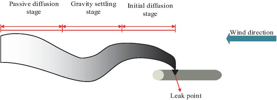
Figure 1 Diagram of SF6 diffusion process.

Figure 1 shows the SF6 diffusion process. Initial diffusion stage, the initial speed of SF6 leakage dominates the starting movement, and the momentum of SF6 leaking out of the pipeline will directly affect the height and distance of air transportation. In the settling stage, gravity exerts a dominant influence on diffusion. The molecular weight of SF6 is greater than that of air, which results in the sinking of SF6. In the passive diffusion stage, the leaked SF6 is gradually diluted, and its density is gradually close to that of the outside air. When the densities of the two are almost equal, the SF6 gravity effect disappears and the heavy air diffusion becomes non-heavy air diffusion. Since SF6 is a continuous incompressible fluid in the NS of CFD, it essentially obeys the momentum, energy, and mass conservation (MC) equations. Equation (9) displays the MC equation.

$$\frac{\partial {\kappa }^{*}}{\partial t}+\frac{\partial ({\kappa }^{*}U)}{\partial x}+\frac{\partial ({\kappa }^{*}V)}{\partial y}+\frac{\partial ({\kappa }^{*}W)}{\partial z}=0$$

(9)

In Equation (9), ${\kappa }^{*}$ denotes the fluid density in kg/m${}^3$. $U$ denotes the velocity vector component in the $x$ direction in m/s. $V$ denotes the velocity vector component in the $y$ direction in m/s. $W$ denotes the velocity vector component in the $z$ direction in m/s. The equation of conservation of momentum is shown in Equation (3.1).

${\displaystyle \frac{\partial ({\kappa }^{*}U)}{\partial t}}+{\displaystyle \frac{\partial ({\kappa }^{*}UU)}{\partial x}}+{\displaystyle \frac{\partial ({\kappa }^{*}VV)}{\partial y}}+{\displaystyle \frac{\partial ({\kappa }^{*}WW)}{\partial z}}$

$\mathrm{\hspace{1em}\hspace{1em}}={\displaystyle \frac{\partial }{\partial x}}\left(\mu {\displaystyle \frac{\partial U}{\partial x}}\right)+{\displaystyle \frac{\partial }{\partial x}}\left(\mu {\displaystyle \frac{\partial V}{\partial y}}\right)+{\displaystyle \frac{\partial }{\partial x}}\left(\mu {\displaystyle \frac{\partial W}{\partial z}}\right)-{\displaystyle \frac{\partial p}{\partial x}}+S_U$

(10)

In Equation (3.1), $p$ denotes the pressure acting on the fluid microelement in Pa. $S_U$ denotes the generalized source term. Equation (3.1) displays the energy conservation equation.

${\displaystyle \frac{\partial ({\kappa }^{*}{T}^{*})}{\partial t}}+{\displaystyle \frac{\partial ({\kappa }^{*}U{T}^{*})}{\partial x}}+{\displaystyle \frac{\partial ({\kappa }^{*}V{T}^{*})}{\partial y}}+{\displaystyle \frac{\partial ({\kappa }^{*}W{T}^{*})}{\partial z}}$

$\mathrm{\hspace{1em}\hspace{1em}}={\displaystyle \frac{\partial }{\partial x}}\left({\displaystyle \frac{\kappa }{C_p}}{\displaystyle \frac{\partial T^{*}}{\partial x}}\right)+{\displaystyle \frac{\partial }{\partial y}}\left({\displaystyle \frac{\kappa }{C_p}}{\displaystyle \frac{\partial T^{*}}{\partial y}}\right)+{\displaystyle \frac{\partial }{\partial z}}\left({\displaystyle \frac{\kappa }{C_p}}{\displaystyle \frac{\partial T^{*}}{\partial z}}\right)+S_{T^{*}}$

(11)

In Equation (3.1), $\kappa$ denotes the fluid heat transfer coefficient in W/(m${}^2\cdot$K). $T^{*}$ denotes absolute temperature in $K$. $S_{T^{*}}$ denotes viscous dissipation. Turbulence models include the standard $k-\epsilon$, renormalization group (RNG) $k-\epsilon$, and realizable $k-\epsilon$ models. The equation of Standard $k-\epsilon$ is expressed as shown in Equation (12).

$$\frac{\partial }{\partial t}({\kappa }^{*}\kappa )+\frac{\partial }{\partial x_i}({\kappa }^{*}\kappa {\delta }_i)=\frac{\partial }{\partial x_j}\left[\left(\delta +\frac{{\delta }_i}{{\sigma }_k}\right)\frac{\partial \kappa }{\partial x_j}\right]+G_k+G_b-{\kappa }^{*}\epsilon -Y_m$$

(12)

In Equation (12), ${\delta }_i$ denotes the average fluid velocity in m/s. $\delta$ denotes the fluid viscosity coefficient. $\epsilon$ denotes the dissipation rate. ${\sigma }_k$ denotes the coefficient of $k$ equation. $Y_m$ denotes the change in the total dissipation coefficient due to pulsating expansion in compressible flow. $G_b$ denotes the turbulent kinetic energy that emerges from buoyancy. The $k-\epsilon$ model is usually used in fluid calculations with high stability and accuracy. However, the model is a semi-empirical formulation and is only applicable to fully developed turbulent flows. The RNG $k-\epsilon$ model is obtained based on the $k-\epsilon$ model diffusion, and the specific equations of this model are shown in Equation (13).

$$\frac{\partial ({\kappa }^{*}\kappa )}{\partial t}+\frac{\partial ({\kappa }^{*}\kappa {\delta }_i)}{\partial x_i}=\frac{\partial }{\partial x_j}\left[{\alpha }_k{\mu }_{\mathit{eff}}\frac{\partial K}{\partial x_j}\right]+G_k-{\kappa }^{*}\epsilon$$

(13)

In Equation (13), ${\alpha }_k$ takes the value of 0.39. ${\mu }_{\mathit{eff}}$ denotes the sum of the average velocity of the fluid and the viscosity coefficient of the fluid. The RNG $k-\epsilon$ model incorporates the effect of eddies on turbulent flow and improves the computational accuracy of predicting cyclonic flow. The realizable $k-\epsilon$ model is also obtained based on the $k-\epsilon$ model diffusion, and the specific equations of this model are shown in Equation (14).

$$\frac{\partial ({\kappa }^{*}\kappa )}{\partial t}+\frac{\partial ({\kappa }^{*}\kappa {\delta }_i)}{\partial x_i}=\frac{\partial }{\partial x_j}\left[\left(\delta +\frac{{\delta }_i}{{\sigma }_k}\right)\frac{\partial K}{\partial x_j}\right]+G_k-{\kappa }^{*}\epsilon$$

(14)

Equation (14) contains the relevant conditions to satisfy the constrained Reynolds stress, which can ensure the consistency between the model and the actual turbulent flow in terms of Reynolds stress. SF6 leakage does not contain chemical reactions, so only the component transport equation is needed, and its MC equation is shown in Equation (3.1).

${\displaystyle \frac{\partial ({\kappa }^{*}{C}_s)}{\partial t}}+{\displaystyle \frac{\partial ({\kappa }^{*}U{C}_s)}{\partial x}}+{\displaystyle \frac{\partial ({\kappa }^{*}V{C}_s)}{\partial y}}+{\displaystyle \frac{\partial ({\kappa }^{*}W{C}_s)}{\partial z}}$
$\mathrm{\hspace{1em}\hspace{1em}}={\displaystyle \frac{\partial }{\partial x}}(D_s,{\displaystyle \frac{\partial ({\kappa }^{*}{C}_s)}{\partial x}})+{\displaystyle \frac{\partial }{\partial y}}(D_s,{\displaystyle \frac{\partial ({\kappa }^{*}{C}_s)}{\partial y}})$
$\mathrm{\hspace{1em}\hspace{1em}}\mathit{\hspace{1em}}+{\displaystyle \frac{\partial }{\partial z}}(D_s,{\displaystyle \frac{\partial ({\kappa }^{*}{C}_s)}{\partial z}})$	(15)

In Equation (3.1), $C_s$ is the mass fraction of SF6 in the GM. $D_s$ is the DC of SF6 in the GM.

3.2 Finite Volume Method and Physical Modeling

Factors affecting gas leakage are categorized into intrinsic and extrinsic factors. Since SF6 gas leakage occurs inside the substation, the influence of external environment on SF6 leakage can be basically ignored. The intrinsic factors are the influence of SF6 gas itself, including gas density, leakage state, leakage location and leakage port. The relative density of the gas can be judged by the size of the gas in the leakage process is mainly affected by which kind of force. The gas is mostly impacted by gravity when the gas leak starts to spread since the gas density is higher than the air density. Additionally, the gas that accumulates on the ground as a result of gravity causes the concentration of gas to leak fast in the plane near the ground. The principal factor affecting a gas whose density is lower than that of air is buoyancy. This causes the gas to rise and migrate away from the ground, raising the concentration of the gas away from the ground plane. Leakage sources can be categorized into continuous and transient leakage sources based on the state of leakage. The size and shape of the leakage opening affects the gas diffusion process. The amount of gas that leaks out of a leakage opening per unit of time increases with its size, which also increases the LMFR and the concentration of the leaking gas. When the leaking port has a circular form, the LMFR is maximum. The concentration of the leaking gas near the ground increases with leak proximity to the earth. The concentration of leaking gas close to the ground decreases as the leak moves farther away from the surface. While SF6 gas with a volume concentration exceeding 1000 parts per million is safe for human respiration in enclosed spaces, pure SF6 gas is not. Consequently, the study employs the finite volume approach to ascertain that 1,000 ppm represents the threshold concentration of SF6 gas. This concentration is deemed to have reached a dangerous level when it exceeds 100 ppm within the substation room. This study is based on the LMFR and leakage diffusion models. FLUENT software is used to simulate SF6 leakage in substations. The leakage outlet model for substations is shown in Figure 2.

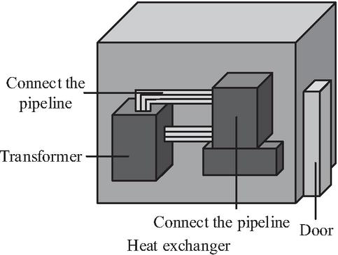
Figure 2 Substation leakage port model.

Figure 2 shows the physical model of the leakage port of a substation. The study constructs a three-dimensional model based on the actual physical model of a substation. The three-dimensional model of the substation is meshed. The division results are shown in Figure 3.

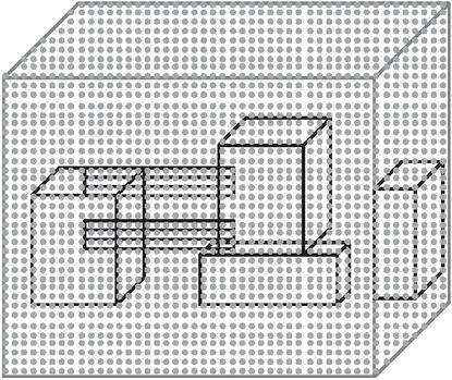
Figure 3 Grid division results of substation model.

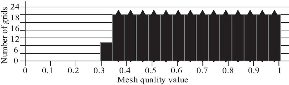
Figure 4 Grid quality check result.

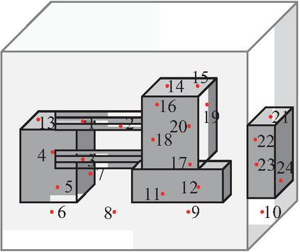
Figure 5 The monitoring point positions.

Figure 3 shows the result of substation mesh division. The number of meshes after division is 2465979 and the number of nodes is 453156. The mesh quality needs to be checked after division and the result of checking is shown in Figure 4.

Figure 4 shows the results of the grid quality check. The X-axis represents the grid quality value, which is dimensionless and has a value range of 0 to 1. The closer the value is to 1, the more regular the grid shape is. The number of grids corresponding to the quality interval on the Y-axis. After checking, the quality of the smallest grid cell is greater than 0.2, which meets the NS requirements. In this study, 24 monitoring points are set up indoors in the substation. Since SF6 is a heavy gas that accumulates on the ground and can form vortices and concentration blind zones, vertical and horizontal stratification are carried out when designing the layout of the monitoring points. First, vertical stratification is carried out. Then, twelve points are set up in each of two planes: the near-surface layer and the human respiratory layer. The initial settlement of SF6 and its accumulation near the ground are monitored through the near-surface layer. The exposure risk to staff is evaluated through the human respiratory layer. Then, horizontal stratification is carried out and the substation equipment layout is divided into three types of areas: an equipment-dense area, a passage area, and a corner blind area. Among them, 8 points are set in the equipment-dense area, 10 points in the passage area, and 6 points in the corner blind spots. Finally, through flow field simulation, it should be ensured that the monitoring points cover the high-incidence area of vortices and the air flow channel area. The wind speed in the high-incidence area of vortices is less than 0.2m/s, and the wind speed in the air flow channel area is greater than 1m/s. At the same time, it is ensured that the distance between adjacent detection points does not exceed 3m to avoid blind spots. Figure 5 shows the layout of the monitoring points.

Figure 5 shows the detection point setup in the substation room. The monitoring points are set at two planes of 0.1 m and 1.5 m. The reason is that SF6 gas is denser than air and the breathing plane of most people is about 1.5 m from the ground.

4 SF6 Leakage Early Detection Modeling Results Study

Leakage port diameter (LPD) and leakage locations are selected as variable parameters to study the leakage of SF6 under different parameters.

4.1 Leakage Port Diameter Impact Analysis

The study selects LPDs of 2 mm, 10 mm and 20 mm for analysis and comparison, while the specific setup location of the monitoring point in the substation room is shown in Table 1.

Table 1 Monitoring point coordinates

Monitoring	Concrete	Monitoring	Concrete
Point Locations	Coordinates	Point Locations	Coordinates
Point 1	(0.1,0.1,1.5)	Point 13	(6,5,1.5)
Point 2	(0.1,5,1.5)	Point 14	(6,9.9,1.5)
Point 3	(0.1,9.9,1.5)	Point 15	(4,0.1,0.1)
Point 4	(4,0.1,1.5)	Point 16	(4,5,0.1)
Point 5	(4,5,1.5)	Point 17	(4,9.9,0.1)
Point 6	(4,9.9,1.5)	Point 18	(7.9,0.1,0.1)
Point 7	(0.1,2.5,1.5)	Point 19	(7.9,5,0.1)
Point 8	(0.1,7.5,1.5)	Point 20	(7.9,9.9,0.1)
Point 9	(2,0.1,1.5)	Point 21	(6,0.1,0.1)
Point 10	(2,5,1.5)	Point 22	(6,5,0.1)
Point 11	(2,9.9,1.5)	Point 23	(6,9.9,0.1)
Point 12	(6,0.1,1.5)	Point 24	(7.9,7.5,0.1)

Table 1 shows the specific coordinates of the 24 monitoring points. Among the 24 monitoring points, Point 1, Point 6, Point 12, Point 15, and Point 21 are selected as the main monitoring points. When the LPD is 2 mm, the diffusion of SF6 is shown in Figure 6.

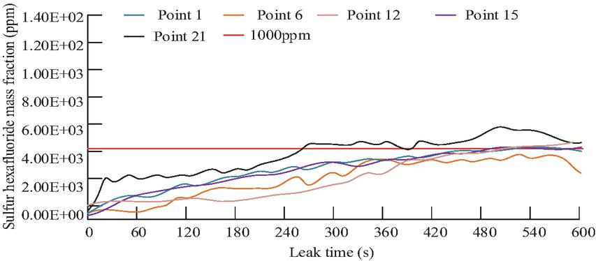
Figure 6 Variation of SF6 gas mass fraction.

The SF6 gas mass fraction variation is depicted in Figure 6. This chart shows that the SF6 mass fraction increases quickly at first and then more gradually. When the LPD is 2 mm and the leakage time is 400 s, the volume concentration of SF6 at point 21 exceeds 1000 ppm. When the leakage event is within 10 s, the SF6 concentration of the substation room is far less than 100 ppm. When the leakage time is within 240 s, the SF6 concentration of the monitoring points is far less than 1000 ppm. Due to the continuous leakage of SF6, when the leakage time is 600 s, the vast majority of the monitoring points SF6 concentration exceeds 1000 ppm, indicating that at this time, the SF6 concentration of the monitoring points exceeds 1000 ppm. When the leakage time is 600 s, the SF6 concentration at the majority of the monitoring points is above 1000 ppm, indicating that the SF6 concentration in the majority of the area near the ground in the substation room is above 1000 ppm at this time. When the LPD is 10 mm, the diffusion of SF6 is as shown in Figure 7.

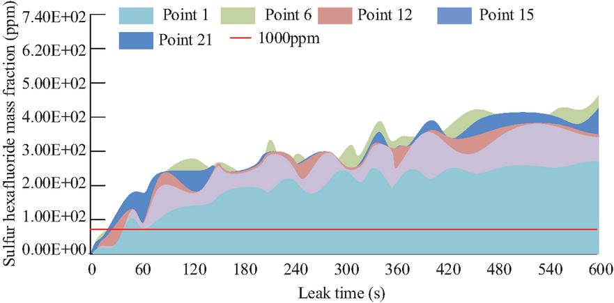
Figure 7 Variation of SF6 gas mass fraction.

Figure 7 shows the variation of SF6 gas mass fraction. The SF6 mass fraction increases rapidly from 0 to 360 s and slowly from 360 s to 600 s. When the leakage time is 360 s, the system tends to stabilize. At a leakage time of 7 s, Point 6 has an SF6 concentration of more than 1000 ppm. Compared with the LPD of 2 mm, the leakage port of 10 mm has a larger LMFR. After a short leakage time, the SF6 concentration in the area closer to the ground is greater than 1000 ppm. When the leakage time is 120 s, the SF6 concentration in most of the area inside the substation room is more than 1000 ppm. The diffusion of SF6 when the LPD is 20 mm is shown in Figure 8.

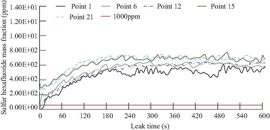
Figure 8 Variation of SF6 gas mass fraction.

Figure 8 shows the change of SF6 gas mass fraction. SF6 mass fraction increases more rapidly in 0–240 s, and the increase slows down in 240 s–600 s. When the leakage time is 240 s, the SF6 mass fraction tends to stabilize. When the leakage time is 5 s, due to the larger LPD, the SF6 concentration in part of the indoor area exceeds 1000 ppm. When the leakage time is 10 s, due to the accumulation of SF6 on the ground after leakage, the SF6 concentration in the area nearer to the ground basically exceeds 1000 ppm. When the leakage time reaches 60 s, most of the interior space has an SF6 concentration higher than 1000 ppm. Concentration of SF6 is more than 1000 ppm. The SF6 diffusion of 2 mm, 10 mm, and 20 mm leak port diameters are counted. Moreover, the results are statistically analyzed through one-way analysis of variance, with the significance level set at 0.05. If $p<0.05$, the differences between groups are significant. If $p>0.05$, there are no significant differences between groups. The results are shown in Figure 9.

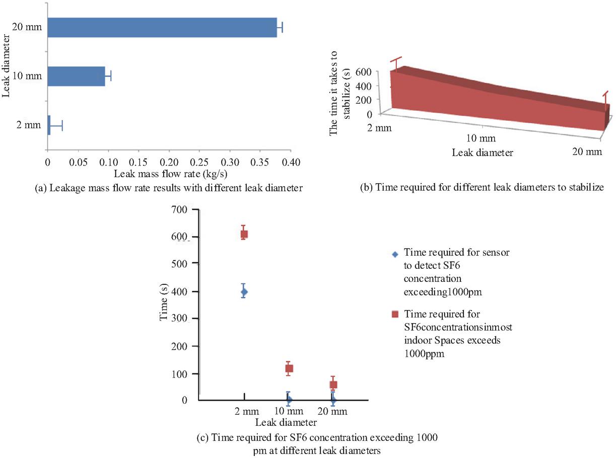
Figure 9 Leakage and diffusion times of SF6 with different leak diameters.

The SF6 diffusion findings for various leakage port widths are displayed in Figure 9. The LMFR for various leakage port sizes is displayed in Figure 9(a), and the data in the figure indicates that the LMFR increases with LPD. The SF6 LMFRs of 2 mm, 10 mm, and 20 mm diameter leakage ports are $0.004\pm 0.0003$ kg/s, $0.094\pm 0.005$ kg/s and $0.377\pm 0.012$ kg/s, respectively. One-way analysis of variance shows that there is a significant difference in the LMFR of SF6 with different diameter leakage ports ($p<0.05$). Figure 9(b) shows the time required for stabilization for different LPDs, and the time for SF6 leakage stabilization is shorter with the increase of LPD. The time to stabilize the SF6 diffusion region is $540\pm 18$ s, $360\pm 12$ s and $240\pm 9$ s for 2 mm, 10 mm and 20 mm diameter leaks, respectively. One-way analysis of variance shows that there are significant differences in the stabilization time required for leakage ports of different diameters ($p<0.05$). Figure 9(c) shows the time required for the SF6 concentration to exceed 1,000 ppm in most of the indoor spaces. The time it takes for SF6 to surpass 1000 ppm in the majority of the substation’s interior space decreases with increasing LPD, and the differences between groups are significant ($p<0.05$). This study conducts a sensitivity analysis to verify the influence of the proposed model on parameter variations. Three parameters, namely leakage aperture, leakage location and SF6 mass flow rate, are selected to analyze their influence on the diffusion effect of SF6 gas. The results are shown in Table 2.

Table 2 Sensitivity analysis

		Diffusion	Diffusion	Concentration	Time to Reach
	Variation	Speed	Range	Accumulation	Hazardous
Parameter	Range	(m/s)	(m${}^3$)	(ppm/s)	Concentration (s)
Orifice diameter	2 mm	0.32	1.23	0.11	125.3
	5 mm	0.67	2.05	0.22	82.7
	10 mm	0.94	3.52	0.31	61.4
	20 mm	1.18	5.03	0.47	43.2
Leak location	Near ground	0.53	2.56	0.26	78.5
	Near equipment	0.83	3.07	0.37	53.6
Mass flow rate	0.004 kg/s	0.41	1.53	0.17	93.8
	0.094 kg/s	0.76	2.84	0.28	66.3
	0.377 kg/s	1.12	4.56	0.43	46.7

In Table 2, when the leakage aperture increases from 2 mm to 20 mm, the diffusion velocity increases from 0.32 m/s to 1.18 m/s. The diffusion range increases from 1.23 m${}^2$ to 5.03 m${}^2$, and the concentration accumulation velocity increases from 0.11 ppm/s to 0.47 ppm/s. The time to reach the dangerous concentration is shortened from 125.3 s to 43.2 s. As the leakage aperture increases, the diffusion rate, diffusion range, and concentration accumulation rate of SF6 gas all increase, and the time it takes to reach dangerous concentrations decreases. When the leakage point is close to the equipment, the diffusion rate of SF6 gas is 0.83 m/s, the diffusion range reaches 3.07 m${}^3$, the concentration accumulation rate is 0.37 ppm/s, and the time to reach the dangerous concentration is 53.6 s. When the leakage point is close to the ground, the diffusion velocity is 0.53 m/s, the diffusion range is 2.56 m${}^3$, the concentration accumulation velocity is 0.26 ppm/s, and the time to reach the dangerous concentration is 78.5 s. When the leakage location is close to the equipment, the gas diffuses faster, accumulates more easily and quickly reaches a dangerous concentration. When the mass flow rate increases from 0.004 kg/s to 0.377 kg/s, the diffusion velocity rises from 0.41 m/s to 1.12 m/s, the diffusion range expands from 1.53 m${}^3$ to 4.56 m${}^3$, and the concentration accumulation velocity increases from 0.17 ppm/s to 0.43 ppm/s. The time to reach the dangerous concentration is reduced from 93.8 s to 46.7 s. It indicates that as the mass flow rate increases, the diffusion rate, diffusion range, and concentration accumulation rate all increase, while the time it takes to reach dangerous concentrations decreases.

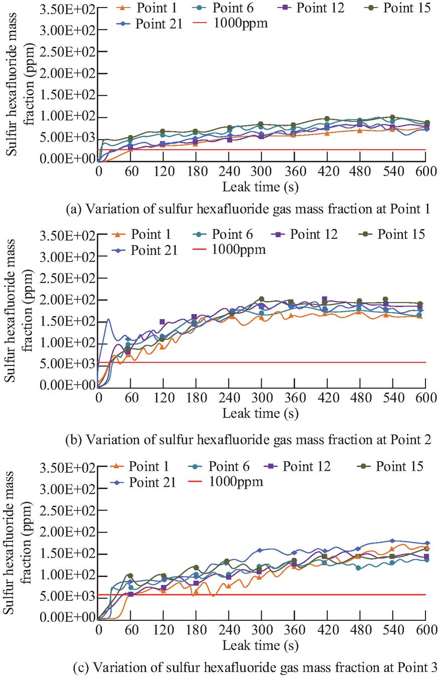
Figure 10 Variation of SF6 gas mass fraction at different leakage locations.

4.2 Leak Location Impact Analysis

Points 1, 2, and 3 are the leakage locations, and the LPD is set at 5 mm. SF6 gas diffusion is depicted in Figure 10 where the leakage locations are Points 1, 2, and 3.

The fluctuation of the SF6 gas mass fraction at various leakage locations is depicted in Figure 10. The change in the SF6 gas mass fraction when Point 1 is the leaking point is depicted in Figure 10(a). When the leakage time is 10 s, the SF6 concentration is more than 1000 ppm in some areas of the transformer room. Figure 10(b) shows the change of SF6 gas mass fraction when the leakage position is Point 2. When the leakage time is 230 s, the SF6 concentration in most areas of the transformer room is more than 1000 ppm. Figure 10(c) shows the variation of SF6 gas mass fraction when the leakage position is Point 3. When the leakage time is 20 s, the SF6 concentration at Point 1 is more than 1000 ppm. The analysis of the SF6 diffusion at various leakage locations is presented in Table 3.

Table 3 shows the SF6 leakage diffusion results at different leakage locations. When SF6 is sprayed vertically downward, SF6 can accumulate on the ground. In addition, the time taken for SF6 concentration to exceed 1000 ppm in most indoor spaces is $120\pm 7$ s, which is higher than that of horizontal spraying. Moreover, in an indoor space 1.5 m from the ground, it takes less than $100\pm 5$ s for the SF6 concentration to exceed 1000 ppm. The leakage diameter, leakage time, and the location of the monitoring point are fitted into the model. One-way analysis of variance shows that there are significant differences in the results of the same indicator in each direction ($p<0.05$). Table 4 displays the obtained error results.

Table 3 Leakage and diffusion of SF6 at different leakage locations

Classification	Point 1	Point 2	Point 3
Leakage gas jet direction	X-axis direction	Z-axis direction	X-axis direction
The time it takes to stabilize (s)	$420\pm 14$	$300\pm 11$	$420\pm 15$
The volume concentration of SF6 in most indoor spaces exceeds 1000 ppm over a period of time (s)	$100\pm 6$	$120\pm 7$	$100\pm 5$
The time required for the concentration of SF6 to exceed 1000 ppm at 1.5m above the floor (s)	$180\pm 9$	$100\pm 5$	$180\pm 8$

Table 4 shows the model error results. the model error is the largest when the LPD is 10 mm and the leakage time is 25 s, at 9.6725 $\pm$ 0.3142 mm. Univariate square difference analysis shows that at the same time, there are significant differences among the results of different diameters ($p<0.05$). This is because under this leakage condition, the gas diffusion rate is relatively fast, and the difference between the model’s predicted value and the actual value is relatively large. Overall, the error value remains within a reasonable range. The proposed model accurately reflects the actual SF6 leakage situation, providing a reliable basis for early warning and emergency response. To verify the application effect of the proposed model in actual scenarios, this study conducts experiments in a 220 kV underground substation in East China. A dual-path infrared SF6 concentration analyzer is used to set up 18 measurement points at the ground and 1.5 m respectively. Steady-state leakage is generated at the valve through reconfigurable micro-pore nozzles. The time to reach 100 ppm when the leakage hole diameters are 2 mm, 10 mm, and 20 mm, the peak density at 1.5 m on the ground, and the maximum lateral diffusion radius (m) are respectively detected. The results are shown in Table 5.

Table 4 Model error result

Time	Diameter (mm)
(s)	2	5	10	15	20
25	$-$7.4563 $\pm$ 0.2847	4.5626 $\pm$ 0.1923	9.6725 $\pm$ 0.3142	5.4612 $\pm$ 0.2216	1.7865 $\pm$ 0.1538
45	4.9822 $\pm$ 0.2431	3.9534 $\pm$ 0.1839	5.1203 $\pm$ 0.2047	3.7521 $\pm$ 0.1714	4.5612 $\pm$ 0.2143
65	3.1454 $\pm$ 0.2208	2.8051 $\pm$ 0.1607	1.4562 $\pm$ 0.1423	1.0278 $\pm$ 0.1241	$-$4.1332 $\pm$ 0.1907
85	1.7096 $\pm$ 0.1536	1.7540 $\pm$ 0.1442	$-$1.7542 $\pm$ 0.1327	$-$1.8642 $\pm$ 0.1621	$-$2.8651 $\pm$ 0.2048
105	0.1251 $\pm$ 0.0827	0.4268 $\pm$ 0.0915	$-$1.7856 $\pm$ 0.1538	$-$3.7410 $\pm$ 0.2337	0.7856 $\pm$ 0.1124
125	$-$2.1243 $\pm$ 0.1742	$-$1.0231 $\pm$ 0.1349	$-$2.0241 $\pm$ 0.1645	$-$5.7802 $\pm$ 0.2541	1.0356 $\pm$ 0.1447

Table 5 Test results of actual scenarios

Leakage Hole	The Time to	Peak Density at 1 m	Maximum Radius of
Diameter (mm)	Reach 100 ppm (s)	Above the Ground (kg/m${}^3$)	Lateral Diffusion (m)
2	18.342 $\pm$ 0.867	0.087 $\pm$ 0.003	2.113 $\pm$ 0.095
10	7.214 $\pm$ 0.354	0.234 $\pm$ 0.007	3.876 $\pm$ 0.141
20	3.926 $\pm$ 0.218	0.411 $\pm$ 0.012	5.049 $\pm$ 0.182

As shown in Table 5, when the leakage aperture increases from 2 mm to 20 mm, the time it takes to reach 100 ppm decreases from 18.342 s to 3.926 s. This indicates that the model can accurately predict when the leakage trigger alarm will sound. The peak density at 1 m ground increases from 0.087 kg/m${}^3$ to 0.411 kg/m${}^3$, indicating that the model can accurately characterize SF6 as the accumulation property of heavy gas. The maximum radius of lateral diffusion increases from 2.113 $\pm$ 0.095 m to 5.049 $\pm$ 0.182 m. This increase proves that the proposed model accurately reflects the influence of the leakage scale on the diffusion range.

5 Conclusion

The study established an SF6 leakage warning model for the SF6 leakage problem in substations. The study first investigated the NS model and analyzed the main factors in SF6 gas diffusion. Then the early warning model was established by combining the finite volume method. The study took a substation room as the research object and set up 24 monitoring points to detect SF6 gas concentration. The results indicated that the SF6 LMFR increased with the increase of leakage diameter. The SF6 LMFR was 0.004 kg/s, 0.094 kg/s, and 0.377 kg/s for 2 mm, 10 mm, and 20 mm diameter leakage ports, respectively. Moreover, the SF6 leakage stabilization time was shorter with the increase of LPD. The SF6 concentration in the substation room was monitored at different leakage locations. Compared with the horizontal injection direction, when the SF6 injection direction was vertical downward, SF6 would pile up toward the ground. Moreover, the time required for the SF6 volume concentration to exceed 1000 ppm in most indoor spaces was 120 s, which was longer than that required for horizontal spraying. Additionally, in indoor spaces at a height of 1.5 meters from the ground, the time required for the SF6 concentration to exceed 1000 ppm was even shorter, at 100 s. The LPD, leakage time, and monitoring point location were incorporated into the model. The maximum error was 9.6725 $\pm$ 0.3142 mm, indicating that the proposed model could more accurately monitor SF6 leakage and provide early warnings. The study’s limitations include the absence of an investigation into the disposal method following the early warning system. The subsequent research can ascertain the emergency disposal measures necessary to mitigate accident hazards.

6 Current and Future Development

In practical applications, the proposed model could be used to add a real-time SF6 concentration data interface to the existing SCADA platform. The 24 monitoring points’ infrared dual-band analyzers could connect to an on-site edge computing server via the IEC 61850 protocol. The server run a lightweight version of FLUENT-UDF that was calibrated for this study. It could predict a rolling three-dimensional concentration field in five seconds. When the measured concentration at any monitoring point reached or exceeded 100 ppm, or the model predicted that the concentration at any point within 600 seconds could reach or exceed 1000 ppm, the system automatically triggered three levels of alarms. The first level triggered an on-site audible and visual alarm and notifies the operator via text message. The second level triggered local exhaust ventilation and closes the air conditioning return air valve. The third level activated all emergency fans, locked the adjacent equipment’s circuit breakers, and triggered the fire emergency broadcast. After an incident occurred, the system automatically compared measured and predicted data, updated the diffusion coefficient, and implemented the model’s online self-learning. While the models and assumptions used in the study may perform well under specific experimental conditions, they may not be applicable to all types of subsurface substations or different leakage scenarios. This study mainly conducts simulations based on a relatively simplified geometric model of the substation, mainly considering the basic spatial structure. The model under review fails to fully incorporate the detailed influence of various densely distributed equipment, obstacles, and their complex layouts on the gas diffusion path and flow field in the actual substation. These factors may cause changes in the diffusion pattern, accumulation area and concentration distribution of SF6. Therefore, a more precise three-dimensional substation layout model will be introduced in the future. This model will facilitate more accurate simulation of SF6 leakage and diffusion behavior in real and complex scenarios. As a result, the practicality and reliability of the early warning model will be further enhanced. At the same time, more flexible and adaptive models can be developed to better handle the complexity in the real environment. Furthermore, studies of long-term stability are essential to assess leak risk and develop coping strategies. Future studies could examine the long-term behavior of SF6 gases under different environmental conditions, as well as how these conditions affect gas diffusion and personnel safety.

Fundings

The research is supported by Science and Technology Project of State Grid Hebei Electric Power CO. LTD (o. kj2022-026).

References

[1] Elmasry Y, Chaturvedi R, Mamun K, Hadrawi S K, Smaisim G F. Numerical analysis and RSM modeling of the effect of using a V-cut twisted tape turbulator in the absorber tube of a photovoltaic/thermal system on the energy and exergy performances of the system[J]. Engineering Analysis with Boundary Elements, 2023, 155(1): 340–350.

[2] Hiremath R, Moger T. Improving the DC-link voltage of DFIG driven wind system using modified sliding mode control. Distributed Generation and Alternative Energy Journal, 2023, 38(3): 715–742.

[3] Moretti L, Simacek P, Advani S G. Efficient numerical modeling of liquid infusion into a porous medium partitioned by impermeable perforated interlayers. International Journal for Numerical Methods in Engineering, 2023, 124(6): 1235–1252.

[4] Corti M, Antonietti P F, Dede’ L, Quarteroni A M. Numerical modeling of the brain poromechanics by high-order discontinuous Galerkin methods. Mathematical Models and Methods in Applied Sciences, 2023, 8(33): 1577–1609.

[5] Li H, Hao T, Li Z, Zhao E, Wang C, Xu L. Research on a self-coordinated optimization method for distributed energy resources targeting risk mitigation. Distributed Generation and Alternative Energy Journal, 2024, 39(3): 659–690.

[6] Mehnert M, Oates W, Steinmann P. Numerical modeling of nonlinear photoelasticity. International Journal for Numerical Methods in Engineering, 2023, 124(7): 1602–1619.

[7] Zhou Z, Li S, Gao X. Numerical modeling of thermal behavior of melt pool in laser additive manufacturing of Ni-based diamond tools. Ceramics International, 2022, 48(10): 14876–14890.

[8] Kunnoth S, Mahajan P, Ahmad S, Bhatnagar N. Compressive strain measurements in porous materials using micro-FE and digital volume correlation. The Journal of Strain Analysis for Engineering Design, 2022, 57(5): 323–339.

[9] El Jery A, Satishkumar P, Salman H M, Khedher K Ml. Comparison of different approaches for numerical modeling of nanofluid subcooled flow boiling and proposing predictive models using artificial neural network. Progress in Nuclear Energy, 2023, 156(2): 104540–104551.

[10] Maranzoni A, Tomirotti M. New formulation of the two-dimensional steep-slope shallow water equations. Part II: Numerical modeling, validation, and application. Advances in Water Resources, 2023, 177(6): 104255–104267.

[11] Park S, Kim M, Koo Y, Kang D, Kim Y, Park J, Ryu C. Numerical modeling of methane pyrolysis in a bubble column of molten catalysts for clean hydrogen production. International Journal of Hydrogen Energy, 2023, 48(20): 7385–7399

[12] Jüngel A, Zurek A. A discrete boundedness-by-entropy method for finite-volume approximations of cross-diffusion systems. IMA Journal of Numerical Analysis, 2023, 43(1): 560–589.

[13] Li Y, Wang Z, Shi X, Fan R. Numerical investigation of the dispersion features of hydrogen gas under various leakage source conditions in a mobile hydrogen refueling station. International Journal of Hydrogen Energy, 2023, 48(25): 9498–9511.

[14] Petersen H I, Smit F W H. Application of mud gas data and leakage phenomena to evaluate seal integrity of potential CO2 storage sites: a study of chalk structures in the Danish Central Graben, North Sea. Journal of Petroleum Geology, 2023, 46(1): 47–75.

[15] Quan L U, Lifeng H, Mengzhu H U. SF6 leakage region enhancement algorithm based on improved HE. Infrared Technology, 2024, 46(4): 437–442.

[16] Zhang L, Liu K, Han H, et al. Dynamic Measurement and Prediction of Sulfur Hexafluoride Gas Weight Based on Non-Ideal Gas State Equation and Improved Random Forest. Journal of Nanoelectronics and Optoelectronics, 2024, 19(4): 451–457.

[17] Kunnoth S, Mahajan P, Ahmad S, Bhatnagar N. Compressive strain measurements in porous materials using micro-FE and digital volume correlation. The Journal of Strain Analysis for Engineering Design, 2022, 57(5): 323–339.

[18] Hao L, Kong D, Wu Y, Liu T, Wang G. Transition and gas leakage mechanisms of ventilated cavities around a conical axisymmetric body. Physical Review Fluids, 2022, 7(12): 123901–123921.

[19] Wang Z, Jiao Z, Liu L. Design and research of power information acquisition system for smart grid. Distributed Generation and Alternative Energy Journal, 2022, 37(2): 185–198.

[20] Liu Y. Finite-volume hyperbolic 3-manifolds are almost determined by their finite quotient groups. Inventiones mathematicae, 2023, 231(2): 741–804.

Biography

Mingle Wei, April 1982, male, Baoding, Hebei province, China. Bachelor’s degree in Computer Science and Technology in 2005, master’s degree in engineering in North China Electric Power University North China Electric Power University Industrial Engineering in 2016.

Working Experience: July 2006–November 2008, China National Grid Cangzhou Power Supply Company; December 2008–October 2009, China National Grid Hebei Electric Academy; November 2009–until now, State Grid Hebei Electric Power CO. LTD.

Academic status: The number of academic papers published 6, the number of academic books published 1, the number of scientific research projects 5, the number of patents 6, the number of academic awards 3.

Distributed Generation & Alternative Energy Journal, Vol. 40_5&6, 1209–1234.
doi: 10.13052/dgaej2156-3306.405612
© 2025 River Publishers