Prediction Model Integrating Attention Mechanism and BP-LSTM Algorithm for Energy Production

Chunxue Zhao^1,*, Guorong Li¹, Xiang Xiao², Chen Song¹ and Jie Yin¹

¹Digital Intelligence Technology Company, Xinjiang Oilfield Company, Karamay 834000, China
²Operation Area of Luliang Oilfield, Xinjiang Oilfield Company, Karamay 834000, China
E-mail: zcx.master@outlook.com
*Corresponding Author

Received 23 June 2025; Accepted 23 June 2025

Abstract

Accurate prediction is crucial for optimizing production plans, improving efficiency, and reducing costs in the energy sector. This study combines a neural network production prediction model with a fusion attention mechanism for energy production. This model uses long short-term memory networks to learn historical production data, integrates back propagation, and introduces attention mechanisms. The results demonstrated that when analyzing different energy sources, the accuracy, the root mean square error, and the prediction time were 0.72, 0.07, and 1.7 seconds, respectively, for a dataset size of 1,000. The proposed model exhibits superior predictive performance across various sources. It provides a more accurate and efficient method for energy production prediction.

Keywords: Attention mechanism, production prediction, BP, LSTM.

1 Introduction

Accurate energy prediction is particularly essential for the energy sector, as in the particular case of oil well production (OWP). Accurately predicting OWP can not only optimize oilfield development plans, but also significantly improve the overall efficiency of oilfield development and reduce operating costs. With the continuous growth of global energy demand and the gradual depletion of oil resources, optimizing oilfield extraction plans and improving oilfield development efficiency have become urgent problems to be solved [1, 2]. The accuracy of OWP directly affects the effectiveness and economy of production decisions. However, traditional prediction methods often struggle to handle complex time-series data, which challenges the accuracy and stability of model predictions. Therefore, it is highly necessary to develop a prediction model that can effectively capture complex dependency relationships in time series data. Therefore, a combination model with fusion Attention Mechanism (AM) is constructed for OWP prediction. This model uses the Long Short-Term Memory (LSTM) to study historical OWP data, combined with Back Propagation (BP) to optimize LSTM, calculate gradients to update model weights, and finally introduces AM to improve the model’s capacity to capture long-distance dependencies.

The innovation of the research lies in addressing the overfitting in traditional LSTM when dealing with small datasets or noisy data. By introducing the BP algorithm to optimize the LSTM model parameters, its performance has been improved. In response to the potential information forgetting and bottleneck issues that may still exist in the BP-LSTM model when processing ultra-long sequences, a convolutional block attention module is introduced to improve the model’s ability to capture remote context by combining channel attention and spatial AMs. Deep learning techniques are applied to OWP prediction, and BP-LSTM and BP-LSTM-ATT models are proposed. The performance advantages are verified on actual datasets. Through various model comparison experiments, the performance of the model is comprehensively analyzed from multiple indicators. Especially in terms of adaptability and efficiency on different dataset sizes and oil well types, the robustness of the model is demonstrated. The contribution of the research lies in the following three points:

Firstly, a LSTM model optimized with BP algorithm is proposed to address the time series prediction of OWP, which can fully utilize long sequence information and effectively alleviate gradient vanishing and overfitting.

Secondly, to enhance the ability to capture dependencies and key features of ultra long sequences, channel and spatial AMs are integrated to form the BP-LSTM-ATT model, which dynamically focuses on the most relevant temporal information.

Thirdly, through testing on public datasets and actual oil well data, this method outperforms traditional methods in terms of accuracy, Root Mean Square Error (RMSE), training and prediction efficiency, providing a more accurate and efficient solution for OWP prediction.

This study aims to provide a more efficient method for predicting OWP, and provide reference for time-series data prediction in related fields.

The paper is organized as follows. The research content is divided into four sections. Section 2 reviews other relevant research topics. Section 3 briefly introduces the main methods used in this study. Section 4 covers the model results obtained by applying the method to the research and analysing the results. The final section summarizes the research and proposes future research areas.

2 Related Works

As the growth of global energy demand and the increasing scarcity of oil resources, optimizing oilfield extraction strategies, improving development efficiency, and reducing costs have become urgent issues to be addressed. Reference [3] constructed a new model integrating SSA and LSTM. The suggested model performed excellently, significantly better than the individual LSTM and SSA-BP models, which was beneficial for the digital safety management of subsea process systems. Reference [4] built a multi-layer model to observe the viscosity of diluted heavy crude oil. This model could predict viscosity more accurately and performed better than existing models, with a coefficient of determination of 0.95. Reference [5] proposed a permeability model. This model could fully consider the impact of adverse factors on production capacity, providing theoretical guidance for optimizing fracturing in low-permeability reservoirs.

Reference [6] established a three-dimensional numerical model. Meanwhile, an LSTM-BP neural network prediction model was developed. Increasing the velocity or temperature of the heat transfer fluid can shorten the melting time of phase change materials. Machine learning models provide an adaptive new approach for thermal storage design. Reference [7] proposed a hybrid model based on Convolutional Neural Networks (CNN) and LSTM. The model used dual channel images as inputs. This method performed well in identifying four discharge modes, meeting real-time requirements, and verifying the rationality of hyperparameters and model discrimination ability through ablation experiments. Reference [8] suggested a prediction model based on stacked bidirectional LSTM. This model performed well, demonstrating excellent performance. Reference [9] proposed an architecture that combined multi-condition scheduling algorithms with multi-level queues to optimize workflow scheduling of IoT devices in fog/cloud environments. The architecture utilized Common Prefix Exception (CPE) to calculate priorities and LSTM to predict workloads, achieving efficient task allocation. This method significantly improved system throughput and efficiency, increasing throughput by 48.6%, reducing communication costs by 56%, and significantly improving production span, waiting time, and parallelism.

In summary, many scholars focused on yield prediction and have obtained certain results. Although these methods have improved the effectiveness of yield prediction to some extent, there are still issues such as low accuracy and insufficient robustness. Therefore, a BP-LSTM model based on AM is proposed, aiming to provide a reliable method for OWP prediction.

3 Methods

The first section proposes an LSTM oil well prediction model that can extract temporal information to address the difficulty of predicting OWP, and optimizes its parameters through BP. In the second section, AM is introduced to improve the BP-LSTM model.

3.1 OWP Prediction Model with BP-LSTM

OWP is an essential indicator for oilfield development. Accurately predicting oil production can optimize production plans, improve oilfield development efficiency, and reduce production costs. This study takes LSTM, which can extract temporal information, to learn historical OWP. LSTM is a special recursive neural network architecture primarily used for processing and predicting time series data or tasks with sequential dependencies [10, 11]. Traditional recurrent neural networks are susceptible to gradient vanishing or exploding, while LSTM can better preserve and utilize information over long time steps by introducing gating mechanisms. Figure 1 illustrates the structure.

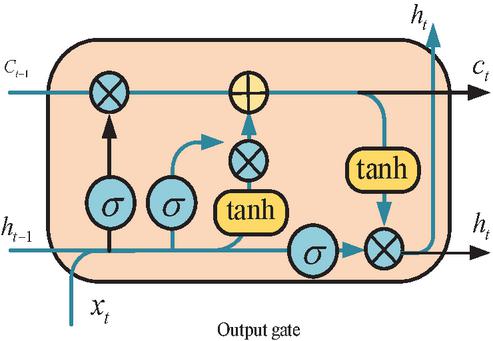
Figure 1 LSTM structure diagram.

In Figure 1, the LSTM is built on CNN, which incorporates a gating structure. LSTM has an additional transitive state compared to CNN, with two transitive states [12, 13]. In LSTM, the updated gate is shown in Equation (1).

z_{t} = σ (W_{z} \cdot [h_{t - 1}, x_{t}])

(1)

In Equation (1), $z_{t}$ denotes the update gate. $W_{z}$ denotes the parameters. $h_{t - 1}$ denotes the hidden state of the previous time step. $x_{t}$ denotes the input of the time step. The output of the reset gate is constrained to the interval [0, 1]. Equation (2) shows the calculation equation of the reset gate.

r_{t} = σ (W_{r} \cdot [h_{t - 1}, x_{t}])

(2)

In Equation (2), $r_{t}$ represents the reset gate. $W_{r}$ represents the parameter. Equation (3) shows the candidate hidden state calculation equation with reset gate calculation.

{\tilde{h}}_{t} = \tanh (W_{h} \cdot [r_{t} ⊙ h_{t - 1}, x_{t}])

(3)

In Equation (3), $⊙$ denotes element wise multiplication. $\tanh$ is the hyperbolic tangent function used to generate new candidate cell states. The hidden state is presented in Equation (4).

h_{t} = (1 - z_{t}) ⊙ h_{t - 1} + z_{t} ⊙ {\tilde{h}}_{t}

(4)

In Equation (4), $h_{t}$ is applied to calculate the next time step. The calculation of hidden states combines output gates with the current unit state. Although the structure of LSTM allows gradients to propagate more smoothly during backpropagation, reducing the gradient vanishing and enabling the network to better learn dependencies with long time steps. However, overfitting is prone to occur when dealing with small datasets or noisy data [14, 15]. Therefore, this study applies the Back Propagation (BP) algorithm to optimize the LSTM and calculates gradients to update the weights of the LSTM. However, since LSTM is a recursive neural network that processes time series data, its backpropagation process needs to consider the time dimension. The improved algorithm model is shown in Figure 2.

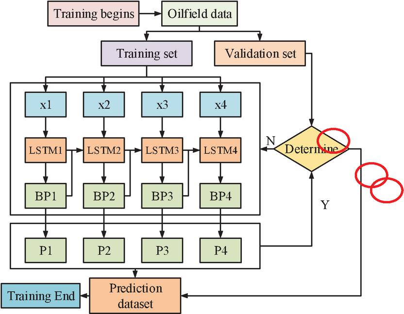
Figure 2 Structure of BP-LSTM.

In Figure 2, the input sequence is sequentially passed through the LSTM unit to calculate the hidden state and cell state, as well as the output of each gate. The loss function is calculated as the optimization objective. Starting from the last time step, the loss of each time step is sequentially calculated [16]. The chain rule is used, where gradients propagate back layer by layer, propagating the loss information. Equation (5) shows the loss function.

Loss = \frac{1}{T} \sum_{t = 1}^{T} L (y_{t}, {\hat{y}}_{t})

(5)

In Equation (5), $y_{t}$ denotes the true value. ${\hat{y}}_{t}$ denotes the predicted value of the model. $L$ represents the loss function. $T$ represents the time step. Equation (6) shows the output gradient corresponding to the loss function.

δ_{y_{t}} = \frac{\partial L (y_{t}, {\hat{y}}_{t})}{\partial {\hat{y}}_{t}}

(6)

In Equation (6), $δ_{y_{t}}$ represents the gradient of the loss function on the output, that is, the impact of the model’s predicted output on the loss. $y_{t}$ represents the output. This gradient represents how the loss will change if the output is changed. The gradient of the output gate is shown in Equation (7).

δ_{o_{t}} = δ_{y_{t}} ⊙ \tanh (C_{t}) ⊙ o_{t} ⊙ (1 - o_{t})

(7)

In Equation (7), $δ_{o_{t}}$ is the gradient of the output gate. $C_{t}$ denotes the cell state. $O_{t}$ represents the output gate. The gradient is calculated through the backpropagation chain, representing the impact of changes in the output gate on the loss. The gradient of the cell state is calculated, as shown in Equation (8).

δ_{C_{t}} = δ_{y_{t}} ⊙ O_{t} ⊙ (1 - \tanh^{2} (C_{t})) + δ_{C_{t + 1}} ⊙ f_{t + 1}

(8)

In Equation (8), the gradient of cell state is calculated through two parts. By selecting feature parameters and daily oil production data, the BP-LSTM model is used to compare the predicted production results with the actual values to predict the OWP.

3.2 OWP Prediction Model with Fusion AM and BP-LSTM

Although BP-LSTM has made significant improvements in handling long-term dependencies compared to LSTM, it may still face difficulties in capturing long-range dependencies when the sequence is very long. As time steps increase, information from early time steps may gradually be “forgotten” or weakened in LSTM, resulting in poor processing of contextual information over long time intervals. In the BP-LSTM architecture, all historical information is compressed into a fixed dimensional hidden state, which leads to information loss or insufficient expression of the complete context [17]. This “information bottleneck” limits the ability to express complex dependency relationships. Therefore, AM is introduced, allowing direct access to remote context without relying on gradually propagating hidden states. This mechanism greatly enhances the ability to capture long-range dependencies, especially when the sequence length is long. By calculating the attention weights of each time step, useful information can be selectively extracted from different time steps according to the current task requirements [18]. This approach breaks the fixed dimensional limitations of hidden states, flexibly utilizing complete contextual information.

AM selectively focuses on specific elements of input data, thereby promoting more efficient information processing within the network. This study employed a Convolutional Block Attention Module Network (CBAM), which is comprised of two principal components: a Channel Attention Module (CAM) and a Spatial Attention Module (SAM). The configuration of the CAM is illustrated in Figure 3.

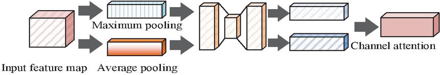
Figure 3 Structure of CAM.

In Figure 3, the maximum pooling feature map and the average pooling feature table are initially obtained. Subsequently, the Sigmoid function is employed to add and activate the feature map, thereby obtaining the final spatial attention feature, which is illustrated by Equation (9).

M_{C} (F) = Sigmoid (F_{\max}^{c,'} + F_{a v}^{c,'})

(9)

In Equation (9), $F_{\max}^{c,'}$ denotes the feature map obtained after global pooling, and $F_{a v}^{c,'}$ denotes the feature map obtained after average pooling. The attention features obtained through the CAM are illustrated in Equation (10).

F_{C} = M_{C} (F) \otimes F

(10)

In Equation (10), $M_{C} (F)$ denotes the final channel attention feature. $F$ denotes the input feature map. Figure 4 illustrates the structure of the SAM.

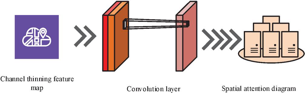
Figure 4 Structure of SAM.

As illustrated in Figure 4, the input feature values are conveyed through the channel dimension, thereby facilitating the acquisition of the maximum and average pool feature values. Subsequently, the data is fed into the convolutional layer, where it is reduced in dimensionality to generate the output feature map. This is then activated by the Sigmoid function to produce the final CAM feature, as illustrated in Equation (11).

M_{S} (F) = Sigmoid (F_{S}^{'})

(11)

In Equation (11), $F_{S}^{'}$ denotes the feature map obtained by dimensionality reduction. The attention feature obtained through the SAM is shown in Equation (12).

F_{S} = M_{S} (F) \otimes F_{C}

(12)

In Equation (12), $M_{S} (F)$ represents the final channel attention feature. $F_{C}$ represents the feature obtained through the SAM. Figure 5 illustrates the final AM structure.

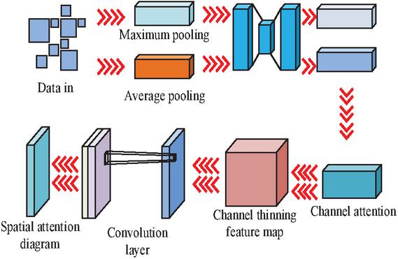
Figure 5 CBAM structure diagram.

In Figure 5, first, the important information from the feature map is extracted and summarized. Then, the pooled feature maps are fed into the CAM, which generates CAM maps by combining the pooling results to determine which channels are more important and adjust their weights. Next, the feature map after channel attention is further refined to highlight the most relevant channels. Subsequently, these refined feature maps undergo more complex pattern detection through convolutional layers. Finally, CBAM applies spatial AM to generate spatial attention maps to determine which position in the feature map owns the essential information. The methodology employed by the model to ascertain the anticipated yield is illustrated in Figure 6.

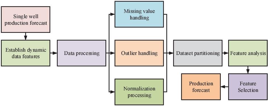
Figure 6 Production prediction process diagram.

In Figure 6, firstly, dynamic data features are established to provide basic data for prediction. The data undergoes a processing stage, which mainly includes handling missing values, handling outliers. Subsequently, the processed dataset is partitioned into a training set and a testing set for the construction and validation of the model. After completing the dataset partitioning, the model begins to perform yield prediction by analyzing different features. Feature analysis is used to help identify the variables that have the greatest impact on the model’s prediction results, ultimately accurately predicting single well production.

4 Results

The first section takes accuracy and RMSE as comparison indicators to analyze the effectiveness of the BP-LSTM. The second section conducts predictive analysis on actual oil wells.

4.1 Performance Analysis of OWP Prediction Model with BP-LSTM

The experimental hardware configuration used in this study included an Intel Core i5-8750H CPU, NVIDIA Geforce GTX2080Ti GPU, 8GB of VRAM, and 16GB of RAM. Due to the relatively dispersed geographical distribution of data for most publicly available OWP forecasting studies, the data sources used by the research institute mainly come from Kaggle’s publicly available oil field production dataset [19]. These data typically focus on typical oilfield blocks in North America or the Middle East, covering key indicators such as daily production, water injection volume, downhole pressure, and wellhead pressure. The dataset contains hundreds to thousands of oil wells. In terms of time span, it generally covers continuous production historical data from several years to more than ten years, providing the possibility for long-term time-series modeling, with a total of 6,000 data points. Due to issues such as missing data, noise, and outliers in raw oilfield data, it is necessary to perform systematic cleaning and transformation before entering model training. The situation where the data recording is particularly incomplete or the oil well has been shut down for a long time has been excluded. In the case of multiple wells, only wells with longer production time spans and higher data integrity can be selected for model training and evaluation. Interpolation filling and other methods are used to complete a small amount of continuous missing production or water injection data. The minimum maximum standardization method standardizes various numerical characteristics including production, injection volume, and pressure.

In the hyperparameter settings of the BP-LSTM-ATT model, the LSTM hidden layer dimension is set to 64, with 2 layers and a Dropout coefficient of 0.2, to balance model capacity and prevent overfitting. The learning rate is set to 0.001, and the Adam optimizer is used in conjunction with a batch size of 32 to balance training speed and stability. The number of training rounds is set to 100, which can be terminated early based on the validation set loss under the early stopping strategy. The channel attention convolution kernel size in the attention module is set to 3 $\times$ 3, with a scaling ratio of 16, and the spatial attention convolution kernel size is set to 7 $\times$ 7. Cross validation and grid search are used to adjust learning rates and other parameters cross validation and grid search to achieve better fitting and generalization performance. Simultaneously, add regularization between each layer of LSTM, with regularization coefficient set to 1e-5, to further avoid overfitting. The batch normalization is adopted to further improve model performance.

In the study, the raw data was first divided into training set, validation set, and testing set in a ratio of 7:2:1. The training set was used for model learning, the validation set was used for real-time monitoring and adjustment of hyperparameters during the training process, and the testing set was only used for final evaluation after the model is finalized. To address the insufficient relative size of the test set, K-fold cross validation is taken to alternate training and validation in different folds, maximizing the utilization of existing data. To verify whether the model is overfitting, evaluation metrics such as accuracy and RMSE are calculated in both training and testing stages, and the difference between the two is monitored. When a model performs well on the training set but fails on the testing set, it indicates that the model may have overfitting. In addition, the Early Stopping strategy is adopted during the training process, which means stopping the training in advance when there is no significant decrease on the validation set for several consecutive epochs, reducing the overfitting. In this way, it is possible to effectively utilize limited data to obtain robust model performance evaluations, as well as identify and suppress overfitting problems by comparing training and testing stage indicators.

In this study, LSTM network, Graph Attention Network (GAT), and Gated Recurrent Unit (GRU) are selected as comparison models, with accuracy and RMSE values chosen as comparison metrics. Figure 7 illustrates the results.

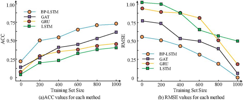
Figure 7 Performance comparison results of four models.

Figure 7(a) showed the accuracy values corresponding to four models, while Figure 7(b) showed the RMSE values corresponding to four models with different dataset sizes. In Figure 7(a), the accuracy values of all four models increased, with the BP-LSTM model having a higher accuracy value among the four models. When the dataset size was 600, the accuracy values of BP-LSTM model, GAT model, GRU model, and LSTM model were 0.62, 0.47, 0.38, and 0.32, respectively. When the dataset size was 1,000, the accuracy values of BP-LSTM model, GAT model, GRU model, and LSTM model were 0.72, 0.63, 0.48, and 0.39. In Figure 7(b), the RMSE values all decreased, with the BP-LSTM model having a smaller RMSE value among the four models. When the dataset size was 1,000, the RMSE values of BP-LSTM model, GAT model, GRU model, and LSTM were 0.07, 0.16, 0.22, and 0.48. Therefore, the BP-LSTM model had good predictive capability. According to the size of the dataset, the training set is divided into four subsets, namely training set 1 to training set 4. Similarly, the validation set is segmented and the computation time was compared. The results are shown in Figure 8.

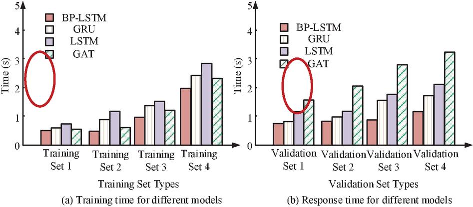
Figure 8 Model training time and validation time.

Figure 8(a) shows the model training time, while Figure 8(b) shows the model running time under different validation set sizes. When the training set was small, the training time of each model was also small. As the training set increased, there was no significant change in the BP-LSTM at the beginning, and then the training time slightly increased. Among the four models, the BP-LSTM remained at a relatively low level. In different validation sets, the multi focus image fusion model maintained a stable computation time as the validation set increased, indicating that the model could handle large amounts of data well, while the computation time of other models increased. As a result, the BP-LSTM model was able to process large amounts of data with high efficiency, demonstrating outstanding efficiency among the four models. Table 1 presents the performance of each model.

Table 1 Comprehensive performance analysis of the model

Index	Dataset	LSTM	GAT	GRU	BP-LSTM
Loss	1	0.298	0.255	0.228	0.165
	2	0.284	0.243	0.214	0.153
IoU	1	0.727	0.769	0.796	0.859
	2	0.745	0.785	0.811	0.875
F1 value	1	0.448	0.491	0.518	0.588
	2	0.489	0.504	0.536	0.594
Micro F1	1	0.799	0.844	0.869	0.933
	2	0.813	0.855	0.883	0.915

In Table 1, IoU is an important indicator for calculating the similarity between two sets. F1 value is an indicator used in classification tasks to comprehensively measure precision and recall. Micro F1 is a F1 value calculation method in multi-classification tasks, which first calculates the global TP FP, FN, and then calculate Precision and Recall again to obtain the F1 value. The loss function values, IoU, F1 value, and Micro F1 of the BP-LSTM algorithm model in dataset 1 were 0.165, 0.859, 0.588, and 0.933, respectively. In dataset 2, the loss function values, IoU, F1 value, and Micro F1 of the BP-LSTM model were 0.153, 0.875, 0.594, and 0.915, respectively. Among the four methods proposed, the BP-LSTM model had excellent performance in all aspects.

4.2 Performance Analysis of Prediction Model with Fusion AM and BP-LSTM

To further validate the performance of the model, the simulation analysis is conducted on each model. In Figure 9, multiple oil well data are selected for predictive analysis.

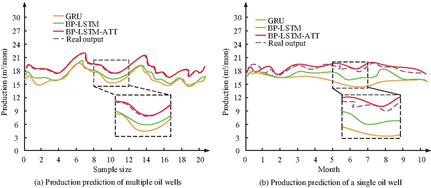
Figure 9 Analysis of predicted values for various models.

Figure 9(a) showed the predicted production for multiple oil wells, while Figure 9(b) showed the predicted production for a single oil well. In Figure 9(a), the performance of each model remained relatively stable as the amount of data increased. Among the four models, the BP-LSTM-ATT model basically fitted the actual OWP, while the GRU model and BP-LSTM model had a large prediction difference. In Figure 9(b), the actual production of each month in a single oil well was basically stable, and the BP-LSTM-ATT model also had good predictive performance, basically fitting around the true value. The other two methods had a significant gap between the models. Thus, the BP-LSTM-ATT had fantastic performance. Different oil wells are selected, and their prediction times are analyzed. The results are shown in Figure 10.

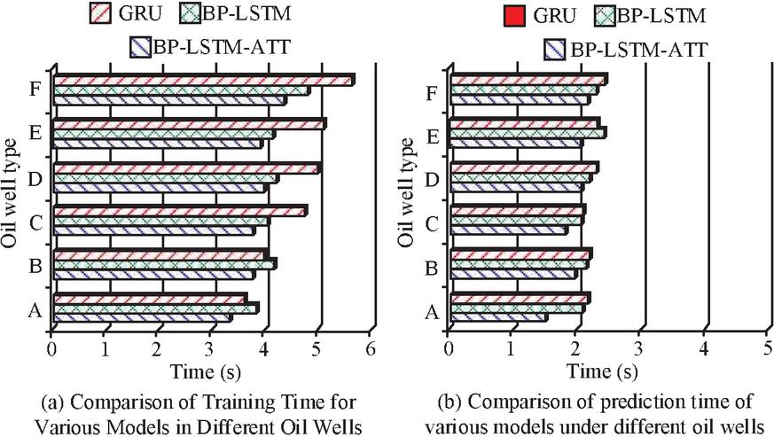
Figure 10 Prediction time for oil wells.

In Figure 10, A to F represented six different oil wells. In Figure 10(a), the BP-LSTM-ATT model had the shortest training time, with training time of 3.1 s, 3.6 s, 4.0 s, 4.3 s, 4.2 s, and 4.5 s for six different types of oil well data, respectively. For different types of oil wells, the training time in Well A was the shortest, with GRU model, BP-LSTM model, and BP-LSTM-ATT model training times of 3.7 seconds, 3.9 seconds, and 3.3 seconds, respectively. In Figure 10(b), among the various models, the BP-LSTM-ATT model had the shortest prediction time, with prediction time of 1.4 s, 1.9 s, 3.6 s, 2.2 s, 2.3 s, and 2.0 s in six different types of oil well datasets, respectively. For different oil wells, the prediction time for C oil well was the shortest, with EGRU model, BP-LSTM model, and BP-LSTM-ATT model having prediction time of 2.1 s, 1.9 s, and 1.7 s, respectively. The BP-LSTM-ATT model had excellent predictive performance for different oil wells. The comprehensive prediction of each oil well is analyzed, and the most advanced model is selected for comparison. The results are shown in Table 2.

Table 2 Comparison of comprehensive production of various oil wells

Oil Well	Actual	GRU			BP-LSTM
Number	Production	Accuracy	RMSE	Production	Accuracy	RMSE	Production
A	13.8	0.737	0.107	10.171	0.819	0.114	11.302
B	17.6	0.843	0.184	14.837	0.883	0.22	15.541
C	15.6	0.877	0.201	13.681	0.902	0.254	14.071
D	21.6	0.803	0.162	17.345	0.865	0.18	18.684
E	23.4	0.832	0.185	19.469	0.888	0.209	20.779
F	16.8	0.888	0.241	14.918	0.944	0.273	15.859
Oil Well	Actual	BP-LSTM-ATT			SOTA
Number	Production	Accuracy	RMSE	Production	Accuracy	RMSE	Production
A	13.8	0.802	0.072	11.068	0.751	0.096	10.3638
B	17.6	0.906	0.138	15.946	0.855	0.162	15.048
C	15.6	0.941	0.155	14.68	0.89	0.179	13.884
D	21.6	0.866	0.118	18.706	0.815	0.142	17.604
E	23.4	0.895	0.141	20.943	0.844	0.165	19.7496
F	16.8	0.959	0.211	16.111	0.908	0.235	15.2544

The accuracy of BP-LSTM-ATT is the highest in most wells, with an accuracy of 0.959 and an RMSE of only 0.211 in well F. Meanwhile, the difference between its predicted production and actual value is small, and the difference between the predicted production of oil well A at 11.068 and the actual production at 13.8 is limited. In contrast, SOTA was slightly inferior overall. Compared with GRU and BP-LSTM, BP-LSTM-ATT showed significant improvement in accuracy in wells A to F, reaching 0.906 and 0.941 in wells B and C, respectively, with lower RMSE. In addition, the predicted production was closer to reality, and the difference between the predicted 15.946 and the actual 17.6 in oil well B is relatively small. The experimental results show that the proposed BP-LSTM-ATT has excellent predictive performance for various types of oil wells, performs the best in comprehensive indicators, and has higher accuracy and stability.

5 Conclusion

To address the poor performance of traditional oil well prediction methods in processing long time series data, a neural network OWP prediction model combining BP-LSTM and fused AM was established. The model learned historical OWP data through LSTM, optimized LSTM using BP algorithm, calculated gradients to update model weights, and finally introduced AM to improve the model’s capability. When the dataset size was 1,000, the accuracy values of BP-LSTM model, GAT model, GRU model, and LSTM model were 0.72, 0.63, 0.48, and 0.39, and the RMSE values were 0.07, 0.16, 0.22, and 0.48. Among the four models, the BP-LSTM-ATT model basically fitted the actual OWP, while the GRU model and BP-LSTM model had a large prediction difference. In the prediction of single well production, the actual monthly production of a single well was basically stable, and the BP-LSTM-ATT model also had good predictive performance, which was basically close to the true value. Among various models, the BP-LSTM-ATT model had the shortest training time, with training time of 3.1 s, 3.6 s, 4.0 s, 4.3 s, 4.2 s, and 4.5 s in six different types of oil well data, respectively. For different types of oil wells, the training time in well A was the shortest, with GRU model, BP-LSTM model, and BP-LSTM-ATT model training time of 3.7 s, 3.9 s, and 3.3 s, respectively. Therefore, compared with traditional prediction models, the BP-LSTM model has significant advantages in handling long-term dependencies and improves prediction accuracy. By introducing the BP-LSTM model with fused AM, the processing capability of long sequence data has been further improved. This model can effectively capture long-range dependencies and significantly improving prediction accuracy. However, there are still certain shortcomings in the research, such as the model stability when dealing with noisy data. Future research can improve algorithms and data preprocessing.

References

[1] Veera Sekhar Reddy B, Rao K S, Koppula N. “An attention based bi-LSTM DenseNet model for named entity recognition in English texts”. Wireless Personal Communications, 2023, 130(2): 1435–1448.

[2] Shiam A A, Redwan S M, Kabir M H, Shin J. “A neural attention-based encoder-decoder approach for English to Bangla translation”. Computer Science Journal of Moldova, 2023, 91(1): 70–85.

[3] Li X, Guo M, Zhang R, Chen G. “A data-driven prediction model for maximum pitting corrosion depth of subsea oil pipelines using SSA-LSTM approach”. Ocean Engineering, 2022, 261(8): 1–7.

[4] Gao X, Dong P, Cui J, Gao Q. “Prediction model for the viscosity of heavy oil diluted with light oil using machine learning techniques”. Energies, 2022, 6(21): 12–26.

[5] Xie Y, He Y, Hu Y, Jiang Y. “Study on productivity prediction of multi-stage fractured horizontal well in low-permeability reservoir based on finite element method”. Transport in Porous Media, 2022, 141(3): 629–648.

[6] Xiao T, Liu Z, Lu L, Han H, Huang X. “LSTM-BP neural network analysis on solid-liquid phase change in a multi-channel thermal storage tank”. Engineering Analysis with Boundary Elements, 2023, 146(12): 226–240.

[7] Zheng Q, Wang R, Tian X, Yu Z, Wang H, Elhanashi A. “A real-time transformer discharge pattern recognition method based on CNN-LSTM driven by few-shot learning”. Electric Power Systems Research, 2023, 219(6): 1–12.

[8] Zhang Y, Cui Z, Liu C, Wang K. “Stacked bidirectional LSTM RNN to evaluate the remaining useful life of supercapacitor”. International Journal of Energy Research, 2022, 46(3): 3034–3043.

[9] Abbasi F B, Rezaee A, Adabi S M A. “Fault-tolerant scheduling of graph-based loads on fog/cloud environments with multi-level queues and LSTM-based workload prediction”. Computer Networks, 2023, 235(10): 1–16.

[10] Chiam D H, Lim K H, Law K H. “LSTM power quality disturbance classification with wavelets and attention mechanism”. Electrical Engineering, 2023, 105(1): 259–266.

[11] Rathore M S, Harsha S P. “Prognostics analysis of rolling bearing based on bi-directional LSTM and attention mechanism”. Journal of Failure Analysis and Prevention, 2022, 22(2): 704–723.

[12] Hsu C Y, Lu Y W, Yan J H. “Temporal convolution-based long-short term memory network with attention mechanism for remaining useful life prediction”. IEEE Transactions on Semiconductor Manufacturing, 2022, 35(2): 220–228.

[13] Zhang L, Wang B, Yuan X, Liang P. “Remaining useful life prediction via improved CNN, GRU and residual attention mechanism with soft thresholding”. IEEE Sensors Journal, 2022, 22(15): 15178–15190.

[14] Li Q J, Ng Y, Wu R R. “Strategies and problems in geotourism interpretation: A comprehensive literature review”. International Journal of Geoheritage and Parks, 2022, 10(1): 27–46.

[15] Zhang B, Xiong D, Xie J, Su J. “Neural machine translation with GRU-gated attention model”. IEEE Transactions on Neural Networks and Learning Systems, 2020, 31(11): 4688–4698.

[16] Li M, Huang P Y, Chang X, Hu J, Yang Y, Hauptmann A. “Video pivoting unsupervised multi-modal machine translation”. IEEE Transactions on Pattern Analysis and Machine Intelligence, 2022, 45(3): 3918–3932.

[17] Li C, Mao Z. “Generative adversarial network-based real-time temperature prediction model for heating stage of electric arc furnace”. Transactions of the Institute of Measurement and Control, 2022, 44(8): 1669–1684.

[18] Mokayed H, Quan T Z, Alkhaled L, Sivakumar V. “Real-time human detection and counting system using deep learning computer vision techniques”. Artificial Intelligence and Applications, 2023, 1(4): 221–229.

[19] Correndo Y S, Carcedo A J P, Secchi M A. “Identifying environments for canola oil production under diverse seasonal crop water stress levels”. Agricultural Water Management, 2024, 302(22): 1024–1030.

Biographies

Chunxue Zhao obtained a master’s degree in Electronic and Communication Engineering from China University of Petroleum (Huadong) in 2015. Currently, she serves as a senior engineer in the information field at the Digital Intelligence Technology Company, Xinjiang Oilfield Company. She has successively led or participated in more than 10 key projects at the level of group companies and oilfield companies, helping the oilfield to increase production and efficiency. At the same time, she has completed the preparation of IoT solutions for 13 oil and gas production units in Xinjiang Oilfield, and led the team to tackle technical research such as low-power narrowband communication, process collaborative simulation, and intelligent early warning for production monitoring. During her work, she has successively achieved 10 provincial and ministerial-level achievements, 5 authorized invention patents, and 8 utility models and software copyrights.

Guorong Li obtained a Bachelor’s degree in Mechanical and Electronic Engineering from China University of Petroleum (Beijing) in 2001. Currently, he serves as a Senior Enterprise Expert at the Digital Intelligence Technology Company, Xinjiang Oilfield Company. His main responsibilities include IoT technology research, solution formulation, project implementation, medium-to-long-term IoT planning, IoT platform construction, and digital-intelligent construction in the new energy sector for Xinjiang Oilfield. Over the past five years, he has been successively awarded the titles of Model Worker and Advanced Scientific and Technological Worker of Xinjiang Oilfield Company. He has also won the Second Prize of Technical Innovation Achievements of the Group Company and the Second Prize of Scientific and Technological Progress of the Oilfield Company. Additionally, he has obtained 2 standard specifications and software copyrights, applied for more than 12 invention patents, and published 5 papers.

Xiang Xiao earned her Bachelor of Engineering degree from Guilin University of Electronic Technology in 2004. She currently serves as a II Engineer in Information Managementat the Luliang Oilfield Operation Area, China National Petroleum Corporation (CNPC) Xinjiang Oilfield Branch. With 20 years of field experience, she possesses extensive expertise in developing software solutions that integrate industrial automation with oilfield production, including: Real-time well safety monitoring systems and Production data analytics tools. She has participated in multiple corporate-level projects and published papers in domestic journals and conference proceedings. Her research focuses on oilfield IoT applications and data modeling.

Chen Song obtained a Bachelor’s degree in Electronic Information Engineering from North China Institute of Science and Technology in 2010. Currently, he serves as a Level 3 Engineer in the Internet of Things (IoT) field at Digital Intelligence Technology Company, Xinjiang Oilfield Company. He has led and participated in more than 10 key projects at the national, group company, and lower levels. He has successively completed the preparation of IoT solutions for 13 oil and gas production units in Xinjiang Oilfield, actively led teams in technical research on low-power narrowband communication, Beidou data transmission, OTS virtual simulation, etc. He has achieved 3 provincial and ministerial-level scientific and technological achievements and patents, with 2 authorized invention patents and 9 utility model patents.

Jie Yin graduated from Wenzhou University with a major in Mechanical Engineering in 2018. She is currently working as an engineer at Digital Intelligence Technology Company, Xinjiang Oilfield Company, mainly responsible for IoT applications and scheme formulation. Up to now, she has been in charge of more than 10 scientific research projects and the formulation of digital transformation schemes.

Distributed Generation & Alternative Energy Journal, Vol. 40_4, 823–844.
doi: 10.13052/dgaej2156-3306.4049
© 2025 River Publishers