Accurate Modeling of Carbon Emissions Under Urban Energy Consumption

Dianjun Wang¹ and Shangyu Wu^2,*

¹Faculty of Social Sciences, University of Nottingham, Nottingham, NG7 2RD, United Kingdom
²Faculty of Business, The University of Sydney, Sydney, 2000, Australia
E-mail: SysysWu@outlook.com
*Corresponding Author

Received 14 July 2025; Accepted 17 September 2025

Abstract

Carbon emissions refer to greenhouse gases, mainly carbon dioxide, released into the atmosphere through human activities or natural carbon cycles. Accurate estimation of carbon emissions helps promote the transformation of social and economic systems toward sustainable development. However, existing methods for estimating carbon emissions have some drawbacks such as low accuracy and large errors. Therefore, this study utilizes two optimization algorithms, namely random search and recursive feature elimination, the stochastic gradient descent optimizer, and regularization techniques, to optimize and improve the gradient boosting decision tree algorithm. On this basis, a carbon emission estimation model for urban energy consumption is constructed. Experimental results show that the model achieves a precision of 98.3%, a recall of 96.3%, an F1 score of 97.9%, an efficiency of 95.7%, a precision error of 0.36%, and a false positive rate of 3.7%. All the above experimental data are superior to the three comparison models. Moreover, the research model still demonstrates strong robustness, generalization and applicability when facing different conditions and scenarios, fully demonstrating the superiority and feasibility of the research model. This provides a new approach for carbon emission estimation under urban energy consumption and contributes to promoting green economic development.

Keywords: Energy consumption, gradient boosting decision tree, optimization algorithms, regularization techniques, carbon emissions.

Introduction

With the intensification of urban energy consumption, carbon emissions have become a critical issue. Accurate estimation of carbon emissions is important for environmental protection [1]. Traditional estimation methods include direct measurement, model calculation, and inventory accounting. Each method has limitations. For example, direct measurement is easily affected by weather and covers only fixed points, making it impossible to cover the entire city [2, 3]. The model calculation method mainly relies on intelligent algorithms to mine the feature relationships of data. The selection of algorithms and parameter Settings directly affect the performance of the determinant. Intelligent algorithms are highly dependent, and their data processing and model iteration take a relatively long time, which easily leads to the problem of lagging results. Meanwhile, the influencing factors of carbon emissions are rather complex, and the algorithm’s ability to capture high-dimensional nonlinear relationships is insufficient, making it difficult for the accuracy to reach the expected goal. A more comprehensive and accurate estimation method is urgently needed [4]. The Gradient Boosting Decision Tree (GBDT) iteratively trains weak classifiers to minimize the loss function, improving estimation quality. It applies to various regression and classification problems [5]. However, when GBDT estimates actual carbon emissions, its adaptability to high-dimensional energy consumption data is relatively weak. It also tends to fall into local optima and has limited accuracy. Combining GBDT with other optimization algorithms can improve estimation performance. Therefore, the research is based on the GBDT framework. The Recursive Feature Elimination (RFE) algorithm, Random Search (RS) algorithm and Stochastic Gradient Descent were introduced respectively. The SGD optimizer optimizes GBDT to obtain a fusion algorithm and uses regularization techniques to improve it to enhance the generalization ability of the fusion algorithm. On this basis, a carbon emission estimation model that fully considers urban energy consumption was constructed. It is expected that it can solve the defects existing in the current estimation methods, and it is expected that the error range of its carbon emission estimation will be smaller than that of the existing estimation models. The innovation of the research lies in the following three points. The first one is to introduce intelligent algorithms and optimizers to optimize the traditional GBDT, thereby obtaining a fusion algorithm. Second, regularization techniques improve the fusion algorithm’s generalization, forming a model targeting urban energy consumption. Third, the model is successfully applied to real problems with promising results.

1 Related Works

GBDT, as an ensemble learning algorithm, excelled at handling nonlinear relationships and high-dimensional data. It iteratively trained each decision tree to fit the residuals of the previous iteration, gradually approaching the optimal solution. Based on this, many domestic and international scholars conducted studies on it. For example, Feng Q et al. proposed an evaluation framework combining Genetic Algorithm with GBDT to improve the accuracy of urban flood risk assessment under frequent flood disasters. They applied weighted estimation on historical data from 16 prefecture-level cities in Shandong Province. The results showed that GBDT achieved higher accuracy and lower errors in identifying urban floods [6]. To address the high computational complexity of traditional exhaustive search in calculating numerous antenna combinations, Yang L’s team proposed an efficient antenna selection algorithm based on GBDT. The algorithm mainly optimized system security capacity and computational complexity. Experiments found that it significantly reduced computational complexity [7]. Facing the problem of low accuracy in transformer fault diagnosis by existing models, Wang L’s group proposed a new transformer fault diagnosis method based on GBDT and introduced intelligent algorithms to optimize GBDT. The results demonstrated that this method had high accuracy, low error, and stable performance [8]. Guo G et al. designed an optimized framework based on GBDT to better capture interaction effects among parameters in the garbage diffusion segment. The framework simulated datasets and established nonlinear mappings to determine interactions among parameters. Results showed a significant improvement in capturing interaction effects [9]. Because current click-through rate prediction methods had low accuracy in handling large-scale data, Zhao B’s team proposed a prediction method combining GBDT with input-aware factorization machines. By refining feature weights of data, the method completed precise prediction. Experiments showed it improved click-through rate prediction accuracy [10].

Currently, research on carbon emission estimation models has made certain progress, and many scholars gradually applied them to practical scenarios. For instance, to estimate real-time carbon emissions of generators more accurately, Liu J’s group proposed a piecewise nonlinear UDEF model. This model fully considered data breakpoints and extremum points to estimate carbon emissions. Results showed it could perform real-time carbon emission and cost estimation for generators [11]. To quantify carbon emissions caused by forest fires in Canada, Byrne B’s team proposed a model based on satellite carbon monoxide observation. They quantified carbon emissions before and after fire occurrences and found that fire-related emissions were comparable to the annual emissions from major fossil fuel-consuming countries [12]. Li T et al. developed a large-scale data-driven framework to accurately quantify carbon emissions of China’s 5G mobile networks. Using collaborative deep reinforcement learning and graph neural networks, they revealed the carbon efficiency trap of 5G networks. The study found that the framework effectively alleviated 5G network carbon emissions [13]. Facing the challenge of reducing greenhouse gases, especially carbon dioxide, Sousa V et al. proposed a carbon emission estimation method based on a new cement production process using mortar. By thermally activating cement slurry, they completed estimation. Results indicated that cement produced by this method had lower carbon dioxide emissions [14]. To better explore the impact of nuclear energy on carbon dioxide emissions in major countries, Pan B’s team proposed a quantile-on-quantile estimator. By considering nonparametric and conventional analyses, the method enhanced unbiasedness and consistency. Experiments showed that nuclear energy and carbon dioxide emissions could estimate and predict each other in most cases [15].

In summary, although research on carbon emission estimation methods has achieved some results, existing methods still face issues such as long estimation periods and poor accuracy. Therefore, this study introduced RFE, RS, and SGD to optimize GBDT, resulting in a fusion algorithm. Regularization techniques are applied to improve the generalization. On this basis, a carbon emission estimation model considering urban energy consumption was constructed. The model aims to estimate carbon emissions accurately under the premise of urban energy consumption and provides a new approach for carbon emission estimation research.

2 The Carbon Emission Estimation Based on Regularization and SGD-RS-RFE-GBDT

2.1 GBDT Structure Optimization Based on RS and RFE

Carbon emission estimation refers to the quantitative calculation of carbon dioxide and other greenhouse gases using scientific methods or intelligent algorithms. The main sources of carbon emissions include energy consumption, industrial production, and waste treatment and the development of renewable energy power generation can reduce carbon emissions [16, 17]. Estimating carbon emissions requires a comprehensive consideration of various factors such as energy structure and population density. GBDT estimates carbon emissions by leveraging its strong ability to fit nonlinear relationships and handle mixed data. The structure of GBDT is shown in Figure 1.

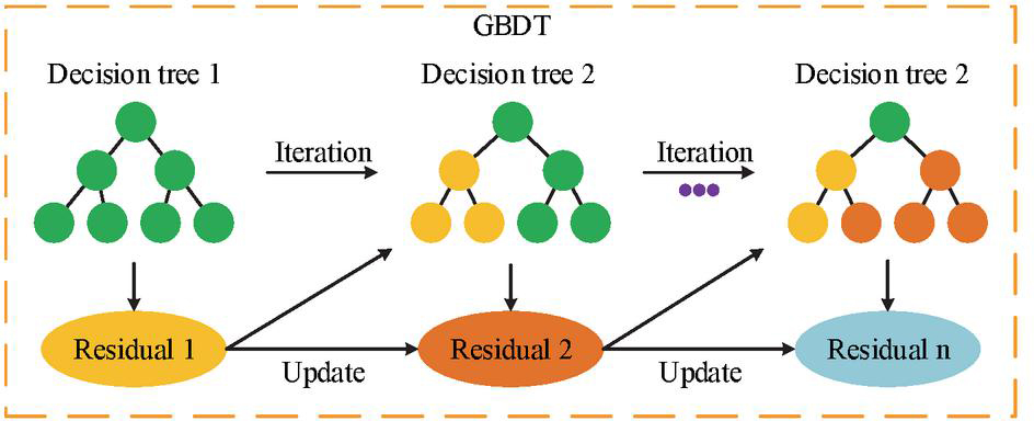
Figure 1 Structure diagram of GBDT (Source from: author self-drawn).

As shown in Figure 1, GBDT, as a decision tree algorithm, builds input data into weak decision trees and fits the residuals of each iteration. Then it enhances data features of the new decision tree based on the previous residuals through gradient boosting. It continues iterating until reaching an optimal solution that meets the conditions. The estimation process of carbon emissions under urban energy consumption using GBDT is shown in Equation (1).

\hat{y} = \sum_{k = 1}^{K} f_{k} (x)

(1)

In Equation (1), $\hat{y}$ represents the estimated value of carbon emissions. $K$ is the number of decision trees. $f_{k} (x)$ indicates the prediction of the $k$ -th decision tree with data $x$ . When estimating carbon emissions from urban energy consumption, GBDT identifies various influencing factors to generate corresponding leaf nodes. This process is shown in Equation (2).

η = \sum_{n = 1}^{n} L (x)

(2)

In Equation (2), $η$ represents the objective function of GBDT. $L (x)$ refers to the loss function of input data $x$ , and $n$ is the number of iterations. However, using GBDT alone may lead to high computational complexity and long estimation periods. Therefore, optimization is necessary. RFE, as a feature selection algorithm, recursively eliminates unimportant features and retains only those that contribute most to the results, thus reducing complexity [18]. This study introduces RFE to optimize GBDT, forming the fusion algorithm RFE-GBDT. Its structure is shown in Figure 2.

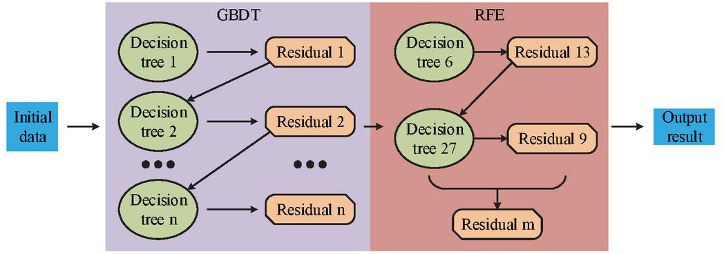
Figure 2 Structure diagram of the RFE-GBDT fusion algorithm (Source from: author self-drawn).

As shown in Figure 2, the RFE-GBDT fusion algorithm first uses GBDT to extract data features and generate decision trees. It then fits the residuals through continuous iteration. Next, RFE removes redundant features – such as unimportant trees and residuals – via recursive elimination, and continues training with the remaining features. This process eventually outputs the best feature set. Each decision tree generated by GBDT contributes to the final result, as shown in Equation (3).

Importance (j) = \sum_{t = 1}^{t} \sum_{i} (i, j)

(3)

In Equation (3), $Importance (j)$ denotes the importance score of feature $j$ . $i$ is the leaf node, and $t$ is the number of iterations. RFE evaluates the remaining features after each elimination step to select higher-quality data features. The process is shown in Equation (4).

δ = \frac{1}{P} \sum_{p = 1}^{P} δ^{(p)}

(4)

In Equation (4), $δ$ defines the evaluation and selection of remaining features by RFE. $P$ represents the number of cross-validations during the evaluation process. However, in the RFE-GBDT hybrid algorithm, the feature selection process of RFE is relatively dependent on the evaluation of feature importance by GBDT. This recursive elimination mechanism is prone to limiting the local optimal solution and still needs to be further optimized. RS generates multiple sets of parameter combinations with certain probabilities in the parameter space and evaluates them to select the best-performing group, thus avoiding local optima [19]. This study introduces RS to optimize RFE-GBDT and forms the fusion algorithm RS-RFE-GBDT. The structure is shown in Figure 3.

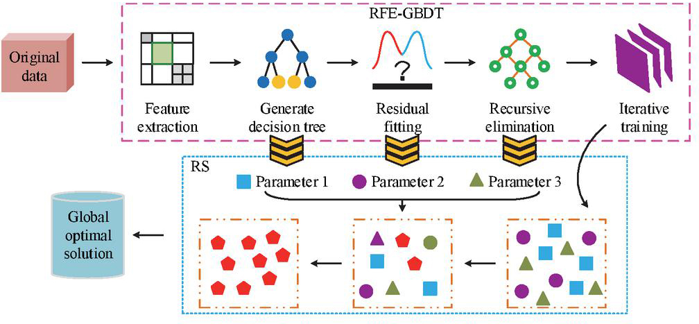
Figure 3 Structure diagram of the RS-RFE-GBDT fusion algorithm (Source from: author self-drawn).

As shown in Figure 3, the unique feature of RS-RFE-GBDT is that RS treats each result from data processing in RFE-GBDT as a parameter group. Then, the RS mechanism filters the results to find the best match. Ultimately, it identifies a globally optimal solution that satisfies all problem constraints. The process of combining parameters based on their distribution is expressed in Equation (5).

Θ = θ_{g} \sim IntegerUniform (c, d)

(5)

In Equation (5), $Θ$ represents the set of parameter groups. $θ_{g}$ refers to one parameter group selected with a probability of $g$ . $c$ and $d$ are data features such as the number of decision trees or residuals. Before RFE removes features, it needs to calculate the importance of each one. This is expressed in Equation (6).

I_{j^{'}} = \sum_{t = 1}^{T} \sum_{b \in j^{'}} (Gini (z) - Gini (z^{'}))

(6)

In Equation (6), $I_{j^{'}}$ denotes the contribution of the $j^{'}$ -th feature. $b$ represents other data features. $Gini (z)$ refers to the Gini impurity of leaf node $z$ before iteration, and $z^{'}$ is the Gini impurity after iteration. Gini impurity is a metric for measuring uncertainty in decision tree algorithms. The function is shown in Equation (7).

Gini (z) = 1 - \sum_{r = 1}^{R} {(\frac{| z_{r} |}{| z |})}^{2}

(7)

In Equation (7), $Gini (z)$ is the Gini impurity. $R$ is the number of parameter categories. $| z_{r} |$ refers to the combination of the $r$ -th category of parameters in leaf node $z$ .

2.2 Carbon Emission Estimation Model Construction Based on SGD and Regularization Improved RS-RFE-GBDT

Although RS-RFE-GBDT has efficient feature selection and extraction ability, high computational efficiency, and good prediction accuracy and generalization, it still lacks strong dependence on temporal data when estimating carbon emissions. As an optimizer used to improve machine learning and deep learning, SGD can enhance the stability and convergence speed of algorithms by iteratively updating their parameters [20]. Therefore, this study improves the RS-RFE-GBDT fusion algorithm using SGD and develops a fusion algorithm that fully considers urban energy consumption, named SGD-RS-RFE-GBDT. Its structure is shown in Figure 4.

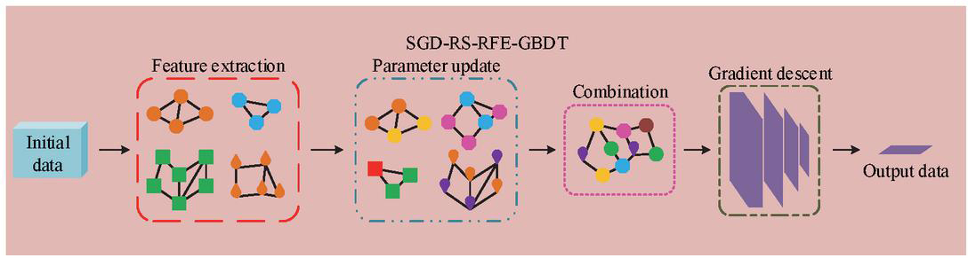
Figure 4 Structure diagram of the SGD-RS-RFE-GBDT fusion algorithm (Source from: author self-drawn).

As shown in Figure 4, the fusion algorithm processes data in four steps. First, GBDT extracts features and constructs decision trees to fit residuals. Second, RFE and RS work together to remove and select features, then optimize parameters to generate new decision trees and residuals. Third, RS generates feature data by randomly selecting parameter combinations. Fourth, SGD uses its specific gradient descent mechanism to select only part of the data in each iteration for gradient calculation and parameter updating, significantly reducing computational complexity and ultimately achieving high-quality data processing. In the fusion algorithm, GBDT generates new decision trees based on the gradient descent mechanism of SGD, as shown in Equation (8).

r^{'} = - [\frac{\partial L (\tilde{y}, y^{k - 1})}{\partial {\tilde{y}}^{k - 1}}]

(8)

In Equation (8), $r^{'}$ represents the negative gradient of the current iteration, $y^{k - 1}$ is the prediction value of the previous $k - 1$ decision trees, and $\tilde{y}$ is the prediction value of the current decision tree. By continuously generating new decision trees, the algorithm produces the best prediction value that satisfies all conditions of the solution, as shown in Equation (9).

y^{*} = {\tilde{y}}^{k - 1} + v \cdot f_{k} (x)

(9)

In Equation (9), $y^{*}$ is the best prediction value. $v$ is the learning rate, with a value range of [0, 1], used to prevent overfitting. When SGD selects part of the data for calculation and updating, it needs to determine the optimization target. Its function is shown in Equation (10).

J (φ) = \frac{1}{n^{*}} = \sum_{n^{*} = 1}^{n^{*}} L^{'} (φ)

(10)

In Equation (10), $J (φ)$ indicates the process of finding the parameter $φ$ to be optimized. $n^{*}$ is the dataset containing all data, and $L^{'} (φ)$ is the loss function. The process by which SGD updates parameters is shown in Equation (11).

φ_{t^{*} + 1} = φ_{t^{*}} - γ \cdot \nabla_{φ} L^{'} (φ)

(11)

In Equation (11), $φ_{t^{*} + 1}$ represents the parameter optimization and update process of SGD during the $t^{*} + 1$ -th iteration. $γ$ is its constraint constant, with a value range of [0, 1]. To improve the generalization ability of the fusion algorithm in estimating carbon emissions, this study applies L1 and L2 regularization to optimize the loss function. The optimization process is illustrated in Figure 5.

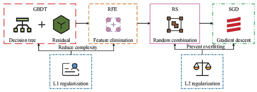
Figure 5 Schematic diagram of the improved loss function using regularization techniques (Icon source from: https://iconpark.oceanengine.com/home).

As shown in Figure 5, the optimization process using regularization techniques includes two parts. The first part applies L1 regularization to constrain the loss function during feature selection, reducing selection complexity and improving effectiveness. The second part uses L2 regularization to restrict the data update and iteration process, preventing overfitting and improving the generalization of the fusion algorithm. The overall loss function optimized by L1 regularization is shown in Equation (12).

L_{1} = L_{loss} + λ \sum_{n = 1}^{n} | ω |

(12)

In Equation (12), $L_{1}$ represents the overall loss function during the feature selection process after L1 regularization. $L_{loss}$ is the original loss function, and $ω$ refers to the feature selection process. The loss function improved by L2 regularization during data updates is shown in Equation (13) [21].

L_{2} = L_{loss}^{'} + \frac{λ}{2} \sum_{n = 1}^{n} ω^{', 2}

(13)

In Equation (13), $L_{2}$ represents the overall loss function of the data update process after L2 regularization. $L_{loss}^{'}$ is the initial loss function, and $ω^{'}$ represents the data update and iteration process. The fusion algorithm optimized by regularization not only has strong feature extraction ability and high computational speed but also avoids overfitting in the final results. Therefore, this study builds a carbon emission estimation model based on the improved SGD-RS-RFE-GBDT fusion algorithm. The overall process is shown in Figure 6.

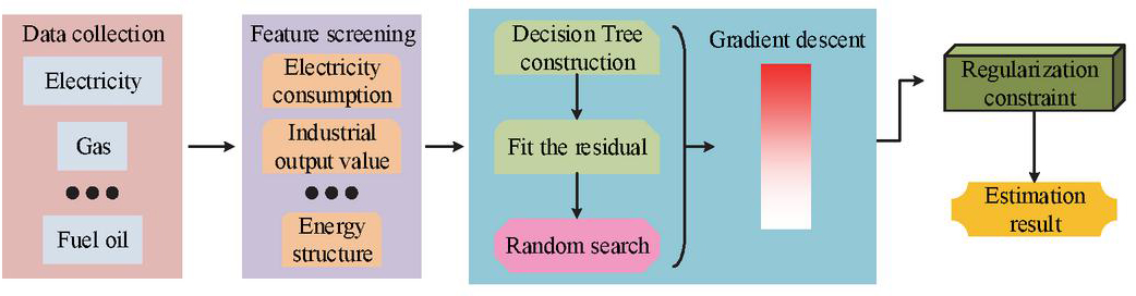
Figure 6 Flowchart of carbon emission estimation under urban energy consumption (Source from: author self-drawn).

As shown in Figure 6, the model estimates carbon emissions under urban energy consumption in seven steps. First, it collects, organizes, and preprocesses the energy consumption data in the city. The second step is to extract the features of energy consumption data through GBDT to construct a decision tree, and then use the recursive feature elimination mechanism of RFE to remove duplicate and reduce noise from the data. After that, RS completes the fitting generation of residuals and the random search of parameter combinations. In the sixth step, SGD optimizes the selected parameter combinations to improve training efficiency. Finally, the regularization techniques constrain the data processing process to avoid overfitting in the estimation results, achieving accurate carbon emission estimation under urban energy consumption.

3 Model Validation for Carbon Emission Estimation Based on SGD-RS-RFE-GBDT

3.1 Performance Testing of SGD-RS-RFE-GBDT

To verify the performance of the SGD-RS-RFE-GBDT fusion algorithm, the study conducted comparative experiments with Convolutional Neural Network and Random Forests (CNN-RF), Improved Support Vector Machine (ISVM), and Graph Convolutional Network and Long Short-Term Memory networks (GCN-LSTM). Among them, ISVM mainly utilizes adaptive kernel functions to improve the traditional SVM, thereby enabling it to dynamically adjust the kernel function parameters according to the distribution of samples. The experimental environment and parameter settings were as follows: the operating system was Windows 11 Professional Edition, the CPU was AMD Ryzen 8845H with a main frequency of 3.8 GHz and the GPU was NVIDIA RTX 4070. The programming language was Python 3.8, the memory was 64 GB DDR5 at 6000 MHz and the storage included a 2 TB solid-state drive and a 2 TB mechanical hard drive. The dataset used was the IEA dataset, which contained statistical data on global energy consumption and carbon emissions. The four algorithms were named Algorithm 1 to Algorithm 4 in the order mentioned above. The study compared the estimation accuracy and error of these algorithms for urban carbon emissions, and the experimental results are shown in Figure 7.

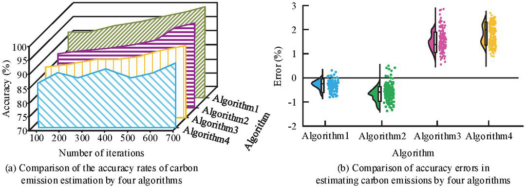
Figure 7 Experimental results of estimation accuracy and error (Source from: author self-drawn).

As shown in Figure 7(a), Algorithm 1 reached a maximum accuracy of 98.3%, which was significantly higher than the 93.5% of Algorithm 2, 89.8% of Algorithm 3, and 86.7% of Algorithm 4. Its average accuracy was 94.7%, also outperforming the other algorithms. Figure 7(b) showed that the estimation error of Algorithm 1 was 0.36%, which was clearly lower than the 0.79% of Algorithm 2, 1.24% of Algorithm 3, and 1.88% of Algorithm 4. This indicated that Algorithm 1 achieved the smallest difference between estimated and actual values, leading to more accurate and reliable results. Next, the study conducted comparative experiments on the memory usage and computational efficiency of different algorithms in carbon emission estimation. The results are presented in Figure 8.

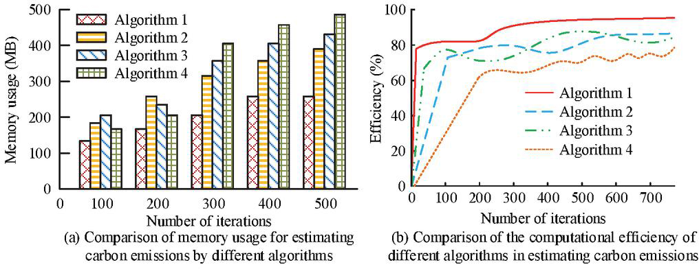
Figure 8 Results of memory usage and computational efficiency (Source from: author self-drawn).

As shown in Figure 8(a), the maximum memory usage of Algorithm 1 during carbon emission estimation was only 241 MB, which was significantly lower than 379 MB for Algorithm 2, 420 MB for Algorithm 3, and 486 MB for Algorithm 4. The memory usage of Algorithm 1 reached its peak at the 400th iteration and remained stable afterward, while the other three algorithms showed a clear increasing trend throughout the process. According to Figure 8(b), the computational efficiency of Algorithm 1 consistently exceeded that of the other algorithms and did not experience any decrease during iterations. In contrast, the other algorithms showed varying degrees of efficiency decline across different iteration intervals. The maximum computational efficiency of Algorithm 1 was 95.7%, noticeably higher than the 85.6% of Algorithm 2, 88.3% of Algorithm 3, and 78.7% of Algorithm 4. In summary, Algorithm 1, which referred to the proposed fusion algorithm, achieved more accurate estimation results and higher performance when estimating carbon emissions under urban energy consumption.

3.2 Effect Validation of Carbon Emission Estimation Model Combining Regularization and SGD-RS-RFE-GBDT

After verifying the performance of the fusion algorithm, the study further evaluated its feasibility through field experiments. The proposed model was compared with the CNN-RF model, the ISVM model, and the GCN-LSTM model. The study selected the capital cities of 34 provincial-level administrative regions in China as the research area and collected their energy consumption data over the past ten years as the original training data. These data were separately input into the four models to estimate carbon emissions, and the results were analyzed and compared. The study first compared the estimation accuracy and F1 score of the four models when dealing with different types of energy consumption. The results are shown in Figure 9.

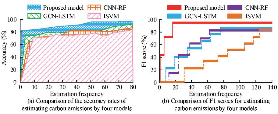
Figure 9 Estimation accuracy and F1 score of carbon emissions (Source from: author self-drawn).

As shown in Figure 9(a), the proposed model reached its maximum accuracy of 96.3% at the 50th iteration and remained stable afterward without significant fluctuations. Its maximum accuracy was notably higher than that of the GCN-LSTM model (89.8%), the CNN-RF model (81.4%), and the ISVM model (77.5%). As seen in Figure 9(b), the F1 score of the proposed model reached its peak of 97.9% within the first 20 iterations, which was significantly higher than the GCN-LSTM model (88.3%), the CNN-RF model (83.7%), and the ISVM model (85.1%). Next, the study conducted a comparative experiment to evaluate the sensitivity of each model when estimating carbon emissions from four sectors: industry, transportation, construction, and residential. The results are presented in Table 1.

Table 1 Sensitivity of carbon emission estimation for different energy consumption types

Energy
Consumption	Experiment	Sensitivity/%
Type	Time	Proposed Model	GCN-LSTM	CNN-RF	ISVM
Industry	Experiment 10	92.2	73.8	80.3	63.8
	Experiment 20	94.6	76.4	83.7	69.2
	Experiment 30	95.3	79.9	86.6	76.5
Transportation	Experiment 10	91.9	82.6	77.0	85.3
	Experiment 20	93.0	83.1	81.2	88.0
	Experiment 30	94.8	85.5	84.9	90.7
Architecture	Experiment 10	93.5	83.0	87.1	79.2
	Experiment 20	92.7	79.7	83.8	83.5
	Experiment 30	94.1	82.4	85.4	87.0
Life	Experiment 10	96.8	88.9	88.2	82.4
	Experiment 20	98.2	90.1	90.4	86.8
	Experiment 30	97.0	89.2	91.5	85.7

As shown in Table 1, the average sensitivity of the proposed model for industrial, transportation, construction, and residential energy consumption was 94.03%, 92.23%, 93.43%, and 97.33%, respectively. All values were higher than those of the three comparison models. In particular, the average sensitivity for residential energy consumption reached a maximum of 98.2%, which was noticeably higher than the values for the other three types of energy consumption. Subsequently, the study randomly added Gaussian white noise to the IEA dataset to test the robustness of the models. By comparing the false positive rate and Mean Absolute Error (MAE) under strong noise conditions, the study assessed how well each model performed. The experimental results were shown in Figure 10.

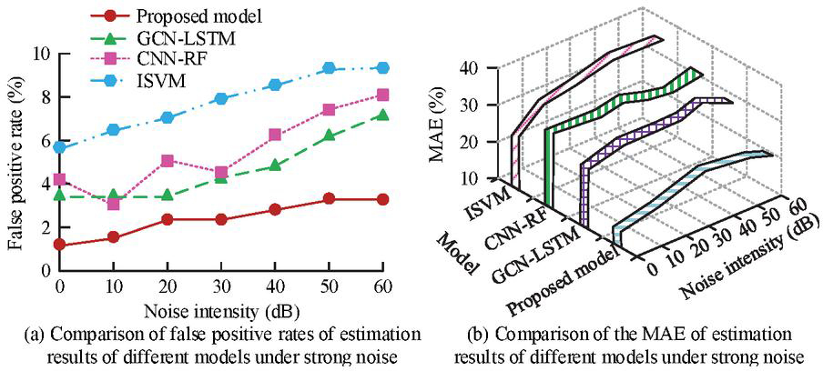
Figure 10 False positive rate and MAE under strong noise interference (Source from: author self-drawn).

As illustrated in Figure 10(a), the proposed model had a maximum false positive rate of only 3.7%, which was significantly lower than that of the GCN-LSTM model (6.9%), the CNN-RF model (8.1%), and the ISVM model (9.6%). Moreover, the false positive rate of the proposed model remained stable in the noise ranges of 20–30 dB and 50–60 dB. According to Figure 10(b), the MAE of the proposed model remained lower than those of the comparison models throughout the experiment. When the noise level was 40 dB, the MAE reached a maximum of 21.4%, which was clearly lower than that of the GCN-LSTM model (29.6%), the CNN-RF model (32.1%), and the ISVM model (34.7%). Additionally, the maximum MAE of the proposed model increased by only 7.2% compared to its initial value, indicating good robustness. Finally, the study introduced the CEADs dataset and conducted comparative experiments on the recall rate of carbon emission estimation using the four models across two different datasets to evaluate their generalization ability. The comparison results were shown in Figure 11.

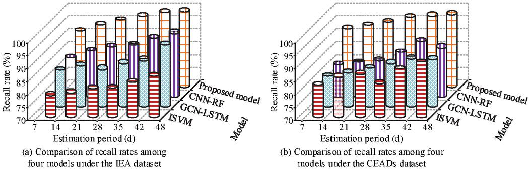
Figure 11 Recall rate of carbon emission estimation across different datasets (Source from: author self-drawn).

In Figures 11(a) and 11(b), the average recall rate of the proposed model was 93.8% on the IEA dataset and 92.7% on the CEADs dataset. These values were significantly higher than those of the CNN-RF model (87.5% and 82.1%), the GCN-LSTM model (84.9% and 80.3%), and the ISVM model (77.3% and 85.7%). Furthermore, the difference in average recall rate for the proposed model between the two datasets was only 1.1%, which was substantially smaller than those of the comparison models. This result demonstrated the strong generalization ability of the proposed model. In conclusion, the proposed model achieved high estimation accuracy and F1 score in estimating carbon emissions under urban energy consumption. It also maintained a low false positive rate and MAE while demonstrating robust performance.

To evaluate the robustness of the research model, the study named this model, the mass balance model, the Transformer-based gated recurrent unit model, and the extreme gradient boosting tree model as Models 1 to 4 in sequence, and deployed them respectively on the Internet of Things terminals in 34 provincial capital cities. The average operating speed and power consumption proportion of 30 carbon emissions estimates under three weather conditions of heavy rain, high temperature and severe cold were evaluated to verify its adaptability to extreme weather. The comparison results are shown in Table 2.

Table 2 Shows a comparison of the average operating speed and power consumption of four models in estimating carbon emissions 30 times under different extreme weather conditions

	Operating Speed/ms				Power Consumption/mW
Weather	Model 1	Model 2	Model 3	Model 4	Model 1	Model 2	Model 3	Model 4
Normal	81.5	50.3	162.4	146.7	32.8	3.5	118.0	84.9
Heavy rain	78.3	47.2	201.9	112.8	34.6	3.7	102.5	73.1
High temperature	86.4	50.8	157.6	131.5	31.0	3.3	120.9	80.7
Severe cold	93.1	48.6	184.5	167.2	35.8	3.4	134.0	92.3

As can be seen from Table 2, since Model 2 estimates carbon emissions based on chemical reaction principles and the law of conservation of materials, without involving neural network calculations or iterative training, and is not affected by extreme weather, it has the fastest running speed and the lowest power consumption. Furthermore, it can be seen from Table 2 that the operating speed and power consumption of Model 1 for estimating carbon emissions under normal weather conditions are 81.5 ms and 32.8 mW respectively, which are the closest to Model 2. The slowest operating speed under severe cold conditions is only 93.1 ms, and the maximum power consumption is as low as 35.8 mW. The fastest operating speed under heavy rain is 78.3 ms, and the minimum power consumption under high temperature is 31.0 mW. Not only is it closer to Model 2, but its adaptability to extreme weather is also significantly better than that of Model 3 and Model 4. This is because the core of the research model is the integrated decision tree, and the reasoning logic is relatively fixed. The fluctuations in energy consumption data caused by extreme weather only change the values input into the model, without increasing the feature dimension or computational complexity. Therefore, its running speed and power consumption are closest to those of the mass balance model.

To analyze the applicability of the research model in estimating carbon emissions of different socio-economic cities under non-Gaussian noise and outlier interference, the study expanded the research area to Nordic cities dominated by renewable energy, and statistically analyzed the energy consumption of 10 representative Nordic cities in the past 10 years. And they were input into models 1 to 4 respectively as the original training data to compare the Mean Absolute Error (MAE) of their estimation of the daily carbon emissions of the city. The experimental results are shown in Table 3.

Table 3 Compares the average absolute errors of each model in estimating the daily carbon emissions of urban energy consumption for 30 times under different experimental groups

	Variable	MAE/%
Experimental Group		Model 1	Model 2	Model 3	Model 4
Data interference	Impulse noise	3.2	11.3	17.6	8.8
	Outlier	2.8	14.0	15.2	7.4
	10% data loss	2.5	15.6	19.0	10.7
Cross-border adaptability	Chinese city	2.7	6.9	14.1	9.5
	Nordic cities	4.6	22.5	20.4	14.3
Socio-economic situation	Benchmark scenario	3.4	5.3	10.7	8.6
	Economic recession	4.0	19.8	16.3	11.4
	Population growth	3.9	14.2	18.5	10.8

It can be seen from Table 3 that the average MAE of Model 1 in the data infection experimental group is 2.83%, which is significantly lower than 16.63% of Model 2, 17.27% of Model 3 and 8.97% of Model 4. The reason lies in that the decision tree structure of Model 1 is not sensitive to noise, and the feature selection of RFE can filter out abnormal features. Meanwhile, regularization can further suppress the influence of interference on the estimation results. For the cross-border adaptability experimental group, Model 1 estimated that the daily carbon emissions of Chinese cities and Nordic cities were both lower than those of the comparison model, and the gap between the two cities mainly consuming different types of energy was only 1.9%. This is mainly attributed to the fact that Model 1, with its feature selection capabilities of RFE and RS, can effectively capture nonlinear features and is less sensitive to structured data than the comparison models. Furthermore, it can be seen from Table 1 that the maximum MAE of Model 1 in the socio-economic scenario experimental group is only 4.0%, which is significantly lower than the minimum MAE value of 5.3% in the comparison model. This is because Model 1 can utilize RFE to screen out key socio-economic features, providing high-quality features for the data processing of GBDT and having a stronger anti-fluctuation ability. By combining the data in Tables 2 and 3, it can be seen that Model 1, namely the research model, has stronger robustness, generalization ability and situational adaptability.

4 Conclusion

To address the problems of low accuracy and high error in existing carbon emission estimation methods, this study optimized the traditional GBDT algorithm using RFE, RS, and SGD. These improvements formed a fusion algorithm named SGD-RS-RFE-GBDT. Regularization techniques were also applied to enhance its generalization ability. Based on this, the study developed a carbon emission estimation model that fully considered urban energy consumption. The proposed model was compared with three existing models, and the results showed that it achieved an accuracy of 98.3% and an efficiency of 95.7%, with an accuracy error as low as 0.36%. Its memory usage was only 241 MB. In field experiments, the proposed model achieved average sensitivities of 94.03%, 92.23%, 93.43%, and 97.33% for industrial, transportation, construction, and residential energy consumption, respectively. It reached an accuracy of 96.3% and an F1 score of 97.9%. Under strong noise interference, the maximum false positive rate was only 3.7%, and the MAE increased by just 7.2% compared to its initial value. In the generalization test, the proposed model achieved average recall rates of 93.8% and 92.7% on the IEA and CEADs datasets, respectively. All of the above experimental results outperformed those of the three comparison models. In addition, the study separately tested the adaptability of the proposed model under five conditions: extreme weather, edge deployment, data interference, urban cross-border, and socio-economic scenarios. The experiments found that the research model was superior to the existing carbon emission estimation models in all cases, fully demonstrating the feasibility and superiority of the research model. Although the model performed well in practical applications, the comparative experiments did not classify the sources of carbon emissions. They only focused on urban energy consumption as a single source. Therefore, future research should explore this limitation further and expand the model to include multiple emission sources.

References

[1] Phoochinda W, Khoasitthiwong B. Guidelines in Local Alternative Energy Management of Communities in Thailand’s Central and Eastern Regions. Distributed Generation and Alternative Energy Journal, 2015, 30(2): 43–56.

[2] Uddin I, Usman M, Saqib N, Makhdum M S A. The impact of geopolitical risk, governance, technological innovations, energy use, and foreign direct investment on CO2 emissions in the BRICS region. Environmental Science and Pollution Research, 2023, 30(29): 73714–73729.

[3] Pata U K, Dam M M, Kaya F. How effective are renewable energy, tourism, trade openness, and foreign direct investment on CO2 emissions? An EKC analysis for ASEAN countries. Environmental Science and Pollution Research, 2023, 30(6): 14821–14837.

[4] Hebbi C, Mamatha H. Comprehensive Dataset Building and Recognition of Isolated Handwritten Kannada Characters Using Machine Learning Models. Artificial Intelligence and Applications, 2023, 1(3):179–190.

[5] Douiba M, Benkirane S, Guezzaz A, Azrour M. An improved anomaly detection model for IoT security using decision tree and gradient boosting. The Journal of Supercomputing, 2023, 79(3): 3392–3411.

[6] Feng Q, Kim H S. Comparative Analysis of Risk Factor Weighting GBDT Methods for Enhancing the Accuracy of Flood Risk Assessment. Journal of the Korean Society of Hazard Mitigation, 2025, 25(2): 9–21.

[7] Yang L, Zhu Q, Ge X, Guo L. Transmit antenna selection for millimeter-wave MIMO system based on GBDT. Journal of Communications and Information Networks, 2023, 8(1): 71–79.

[8] Wang L, Chi J, Ding Y, Yao H Y, Guo Q, Yang H. Q. Transformer fault diagnosis method based on SMOTE and NGO-GBDT. Scientific Reports, 2024, 14(1): 7179–7190.

[9] Guo G, Liu Y, Cao Z, Zhang D, Zhao X. Interpretable GBDT model-based multi-objective optimization analysis for the lateral inlet/outlet design in pumped-storage power stations. Journal of Hydroinformatics, 2024, 26(5): 1189–1205.

[10] Zhao B, Cao W, Zhang J, Gao Y, Li B, Chen F. Fusion of GBDT and neural network for click-through rate estimation. Journal of Intelligent & Fuzzy Systems, 2025, 48(6): 835–847.

[11] Liu J, Zhao H, Wang S, Liu G, Zhao J, Dong Z. Y. Real-time emission and cost estimation based on unit-level dynamic carbon emission factor. Energy Conversion and Economics, 2023, 4(1): 47–60.

[12] Byrne B, Liu J, Bowman K W, Pascolini-Campbell M, Chatterjee A, Pandey S, Sinha S. Carbon emissions from the 2023 Canadian wildfires. Nature, 2024, 633(8031): 835–839.

[13] Li T, Yu L, Ma Y, Duan T, Huang W, Zhou Y, Jiang T. Carbon emissions of 5G mobile networks in China. Nature Sustainability, 2023, 6(12): 1620–1631.

[14] Sousa V, Bogas J A, Real S, Meireles I. Industrial production of recycled cement: Energy consumption and carbon dioxide emission estimation. Environmental Science and Pollution Research, 2023, 30(4): 8778–8789.

[15] Pan B, Adebayo T S, Ibrahim R L, Al-Faryan M A S. Does nuclear energy consumption mitigate carbon emissions in leading countries by nuclear power consumption? Evidence from quantile causality approach. Energy & Environment, 2023, 34(7): 2521–2543.

[16] Li H, Hao T, Li Z, Zhao E, Wang C, Xu L. Research on a self-coordinated optimization method for distributed energy resources targeting risk mitigation. Distributed Generation and Alternative Energy Journal, 2024, 39(3): 659–690.

[17] Hiremath R, Moger T. Improving the DC-link voltage of DFIG driven wind system using modified sliding mode control. Distributed Generation and Alternative Energy Journal, 2023, 38(3): 715–742.

[18] Priyatno A M, Widiyaningtyas T. A systematic literature review: recursive feature elimination algorithms. JITK (Jurnal Ilmu Pengetahuan dan Teknologi Komputer), 2024, 9(2): 196–207.

[19] Reza A A R, Rohman M S. Prediction Stunting Analysis Using Random Forest Algorithm and Random Search Optimization. Journal of Informatics and Telecommunication Engineering, 2024, 7(2): 534–544.

[20] Qin W, Luo X, Zhou M C. Adaptively-accelerated parallel stochastic gradient descent for high-dimensional and incomplete data representation learning. IEEE Transactions on Big Data, 2023, 10(1): 92–107.

[21] Ben Hamida S, Mrabet H, Chaieb F, Jemai A. Assessment of data augmentation, dropout with L2 Regularization and differential privacy against membership inference attacks. Multimedia Tools and Applications, 2024, 83(15): 44455–44484.

Biographies

Dianjun Wang graduated from the University of Nottingham in the UK in 2021. During master’s studies, he compared and analyzed the differences in public policies between China and the UK, dissected the implementation of China’s red line policies, and has certain insights into the implementation and execution of public policies. At present, he is engaged in research on economic policies, the development of digital currencies, urban energy emissions and other fields. He has studied and discussed with government staff and well-known domestic scholars the impact of the urbanization process on green and low-carbon development.

Shangyu Wu graduated from the University of Sydney, Australia in 2021. During her master’s program, she majored in finance and international business courses, and she is currently engaged in financial analysisand risk monitoring. She possesses a profound understanding of financial risk identification and management and is currently conducting in-depth research in this area.

Distributed Generation & Alternative Energy Journal, Vol. 40_5&6, 1259–1280.
doi: 10.13052/dgaej2156-3306.405614
© 2025 River Publishers