Wind Shear Forecasting for Radar Signal Clusters Using Wavelet Transformation and Class Separation Analysis

Ting Xu^1,*, Qionghua Li² and Yan Lu³

¹College of Aviation Meteorology, Civil Aviation Flight University of China, Guanghan, 618307, China
²Jiangxi Air Traffic Management Bureau, Civil Aviation Administration of China, Nanchang, 330114, China
³Heilongjiang Airport Management Group Co., Ltd., Harbin, 150079, China
E-mail: TtxtxtXu@outlook.com
*Corresponding Author

Received 14 July 2025; Accepted 17 September 2025

Abstract

Wind shear (WS) prediction is a critical meteorological challenge that has a major impact on flight safety and radar signal transmission. It remains a key focus in both meteorological and aerospace research. To improve the accuracy of wind shear forecasting, this study proposes a fusion model that combines wavelet transformation with class separation for predicting wind shear within radar signal clusters. The model first utilizes wavelet transformation to extract time-frequency characteristics from radar signals. Subsequently, class separation is applied to assess the separability of signals in the feature space, enabling effective dimensionality reduction and feature selection. The research was carried out using data from Tianfu International Airport, involving 95 radar systems located in various positions. Experimental results demonstrate that the proposed model surpasses other existing models in terms of prediction accuracy, robustness, and generalization capability. When the radar antenna size was set to 30.48 cm, the model achieved a radar radiation intensity of 45 W/m, notably outperforming alternative approaches. Furthermore, under a radar activity level of 400, the model exhibited a low error rate of only $3.5\times {10}^{-3}$, highlighting its precision and stability. The model also maintains consistent performance across diverse environmental conditions, indicating strong adaptability. This study introduces a novel technical approach to enhance the ability of radar signal clustering in wind shear prediction, offering significant practical value in mitigating aviation risks associated with wind shear.

Keywords: Wavelet transformation, class separation degree, signal cluster set, radar signal source, wind shear prediction, feature selection.

1 Introduction

Flight safety is an important theme in the civil aviation industry, and “safety first” has always been the guiding ideology of the civil aviation industry. There are many factors that affect flight safety, including aircraft performance factors, human factors, and flight conditions. According to statistics, aircraft flight conditions are the main factor causing flight accidents. The flight condition mainly refers to the meteorological conditions along the route. Among the atmospheric phenomena that pose a threat to flight safety, low-altitude Wind Shear (WS) is considered the most harmful. It is recognized by the international aviation and meteorological community as an “invisible killer” during aircraft approach and takeoff phases. The biggest hazard of WS is micro-explosion, which has the characteristics of short time and small scale [1, 2]. Wind field prediction can provide an overview of the entire wind field in the airport area at the predicted time, allowing pilots to roughly understand the wind field environment in the airport area at the next time and extract wind speed information on the glide slope from the entire wind field information. Before the WS detection system issues a warning, it can predict possible WS and turbulence, thereby increasing the time interval for pilot response and preparation, greatly reducing the possibility of flight accidents, and improving flight safety and comfort. Therefore, how to monitor WS has become an important research topic [3]. Radar radiation source signals have high penetration capability. Many scholars have proposed that using radar radiation sources for WS monitoring has great potential [4]. Wavelet Transformation (WT) is a time-frequency analysis tool that can effectively extract the time-frequency characteristics of signals. The commonly used implementation methods include numerical integration method, linear frequency modulation Z-transform real (CZT) method, and frequency domain implementation algorithm. The numerical integration method can only be based on wavelets with time-domain expressions, which has limitations in application and cannot be implemented on wavelets with frequency-domain expressions. CZT significantly increases the resource consumption of the system, greatly affecting the hardware implementation of this method. There are issues with storing wavelet spectral coefficients at various scales when implementing algorithms in the frequency domain. To improve the performance of WT, this study first introduces Class Separation Degree (CSD) to evaluate the prediction model, including accuracy and generalization metrics. A WS prediction fusion model combining WT and CSD is proposed, named WTCSDWS.

The technical route of this article is as follows. Firstly, the current research status of WS prediction is analyzed. Then, combining WT and class separation, the pulse coupled signal cluster is analyzed. The reflection intensity of radar radiation source signals is used to monitor WS. Next, the proposed WS prediction model is tested to verify its feasibility. The contribution of the research lies in providing new technological means to enhance the WS prediction ability of radar signal clusters, which helps to improve the environmental adaptability and visibility range of radar monitoring. Meanwhile, it has important practical application value for effectively reducing the risks of flying objects (such as airplanes and drones) during takeoff, landing, and flight. The practical significance of this study lies in improving the environmental response capability of radar detection, thereby expanding the visible range of radar. This study intends to increase the WS prediction level of radar signal sources, thereby avoiding the flight risk of flying objects. The innovation of the research lies in the combination of WT and CSD, which effectively measures the differences between different signal clusters and compensates for the shortcomings of wavelet transform in spatial features. Secondly, a fusion model was constructed, which combines the advantages of wavelet transform and class separation to achieve wind shear prediction of radar signal sources.

The paper is organized into four sections. The first section analyzes and summarizes the current applications of WT and CSD. The second section introduces the connection method between WS and WTCSD and introduces it to the radar signal sources. The third section conducts simulation experiments on the MREQ dataset. The last section analyzes and compares the performance of this system with traditional systems, and points out the shortcomings that still exist in the research.

1.1 Related Works

The WS prediction of radar signal sources based on WT has been widely studied internationally. Yumatov et al. [5] developed a WT method that could objectively record the changes in signal clusters. The experimental model developed made radar signals a new information technology and identified psychological activities based on WT. The experimental results indicated that the main differences could be observed in the signal response. Compared with the correct answer, the data obtained in this study provides a basic possibility for identifying radar states based on wavelet energy calculation during continuous WT. Gowthami et al. [6] proposed a compression method to reduce signal redundancy and the running time of the WT. They believed that only a few methods were effective for radar signals, so reducing the signal size without reducing the signal quality could enhance the inter-system jump speed. The preprocessing module largely suppressed the noise of the input signal, and the proposed encoder compressed heterogeneous data to reduce storage requirements. The experimental results indicated its effectiveness. Singh et al. [7] injected inter-turn faults at the radar to predict the WS of the radar signal source. The inter-turn fault injection could generate surge currents in the network, and fault detection related to surge currents had limitations. These drawbacks prompted researchers to use sample data control to overcome, where WT was used to determine signal types. After injecting faults at the radar signal source, the signal processing speed was faster under the fuzzy logic controller.

With the progress of research, WT cannot adapt to the increasing number of flying objects. Researchers are gradually paying attention to the CSD of radar signal sources. Sun et al. [8] proposed a stack auto-encoder transfer learning method based on category separation and domain fusion to reduce the same data distribution in radar signal clusters. The proposed category separation could indirectly improve the accuracy of the target domain by expanding the differences between categories in the source domain. The effectiveness of the method was validated through the mutual conversion of two public datasets. The experimental results showed that even if there were no labeled fault data in the new machine, the method could achieve 97% signal clustering between different radars. Chui et al. [9] believed that the collected radar signals and time series were influenced by various complex factors, exhibiting multi-component non-stationary patterns. Therefore, the synchronous compression transformation was developed as an empirical mode decomposition tool to improve the time-frequency resolution and energy concentration of multi-component non-stationary signals. This method had mathematical rigor in intermediate frequency estimation, and its effectiveness was demonstrated by experimental results on real datasets. Koldovský et al. [10] proposed an extended independent component and vector method for extracting multi-source signals from time-varying radar signals. Based on the recently proposed hybrid model, they assumed that each source was separate from serial and parallel. This hybrid model allowed for the motion of the desired source, while the separated beamformer remained unchanged. Under the given radar signal cluster model, numerical simulation experiments demonstrated the effectiveness of this study, and superior convergence speed and ability to separate ultra-high-speed signals.

Although existing research on WT and CSD is popular, there are only a few studies that combine these two concepts. This study innovatively links the two, and is significant in predicting the WS of radar signal sources in radar signal clusters.

2 Construction of Radar WS Prediction Model Based on WT and CSD

WT is a signal processing technique that can decompose signals into sub-bands of different frequencies to analyze them. CSD represents the difference between various categories in the feature space, and is an indicator used to measure the radar WS separation between various categories. This study combines the concepts of WT and CSD to conduct cluster analysis on signals to draw more comprehensive conclusions.

2.1 Analysis of Pulse-coupled Signal Clusters Combining WT and CSD

WT can effectively extract the time-frequency characteristics of pulse signals, which are widely used in analysis of pulse-coupled signal clusters. The signal is subjected to wavelet transform to analyze the energy distribution at different frequencies and the distribution of pulse signal clusters at different frequencies to distinguish the time-frequency characteristics of the signal [11]. WT combines time-domain and frequency-domain analysis to decompose the signal into sub-signals of different scales and frequencies, as shown in Equation (1).

$$[1-\delta (k)]*{\parallel x\parallel }_2^2\le {\parallel Ax\parallel }_2^2*[1+\delta (k)]*{\parallel x\parallel }_2^2$$

(1)

In Equation (1), the size of the radar signal segmentation is denoted as $A$. The distance between signals is represented by $\delta (k)$. And $x$ represents the signal in the compressed state. This method can extract the time-frequency characteristics of signals. The chosen wavelet basis function for the study is the Haar function. The decomposition level of WT determines the degree of refinement of the signal being decomposed. The more layers of decomposition, the richer the detailed information of the signal, but the computational complexity will also increase accordingly. Therefore, considering both computational complexity and precision, a 3-layer wavelet decomposition was chosen for the study. Pulse-coupled signal cluster is a complex signal type that includes multiple sub-signal clusters, each of which has multiple pulse signals [12]. The compressed and sparse signals are represented by $x$ and $\theta$, respectively, and their relationship is shown in Equation (2).

$$\{\begin{array}{c}\theta =\alpha x\hfill \\ y=\beta x=\gamma \theta \hfill \end{array}$$

(2)

In Equation (2), the degree of signal dilution is denoted as $\alpha$. $y$ is the predicted value at the end of dilution. $\beta$ and $\gamma$ represent the signal amplitudes before and after dilution, respectively. There are complex interaction relationships between these pulse signals. Therefore, time-frequency characteristics are analyzed and extracted. However, relying solely on WT cannot fully extract all the characteristics of the signal cluster set [13]. Therefore, the study combines CSD to further investigate the signal separation, as shown in Equation (3).

$$\mathit{LI}=\underset{t\to \mathrm{\infty }}{lim}{t}^{-1}*\ln \frac{r_t}{r_0}$$

(3)

In Equation (3), $\mathit{LI}$ represents the degree of signal separation. The degree of signal separation is originally denoted as $r_0$. $t$ represents the time interval. The degree of signal separation at this time is represented by $r_t$. CSD is an indicator used to measure the degree of separation between different signals. In this study, it is used to evaluate the degree of difference between signals in the feature space [14]. CSD first calculates the distance of the signal, and then uses statistical methods to obtain it. In the feature space, a large CSD indicates greater differences between different pulse-coupled signal clusters. The classification effect is better, thus highlighting the differences in signal clusters. The process is shown in Figure 1.

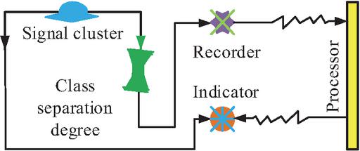
Figure 1 Flow chart of class separation between pulse coupled signal clusters.

As shown in Figure 1, first, signal data is collected or generated to form signal clusters. Then, the CSD between the signal clusters is calculated. The large class separation indicates that there are great differences between different pulse-coupled signal clusters, resulting in better classification performance. Next, the calculated category separation degree is recorded, and an indicator signal is provided based on the result of the category separation degree. Finally, the results of category separation are used to process the signal [15]. Based on the CSD calculation results, the study selects features with high discrimination to evaluate the trained model and test its generalization ability on signals. In actual pulse-coupled signal clusters, different categories of signal clusters need to be automatically separated. The process follows Equation (4).

$$\{\begin{array}{c}\frac{dc}{dt}=\varpi *(j-c)\hfill \\ \frac{dj}{dt}=rc-gc-j\hfill \end{array}$$

(4)

In Equation (4), the scrambled signal cluster set and the initial signal cluster set are denoted as $j$, $c$, and the scaling factor is denoted as $\varpi$, while $r$ and $g$ represent environmental factors, respectively. Then, combining the concepts of WT and CSD, cluster analysis is conducted on the signal. In this process, the study used WT to decompose the signal and extract feature information at different frequencies [16]. The CSD at multiple frequencies is simultaneously calculated to evaluate the difference between sub signals at different frequencies, as shown in Figure 2.

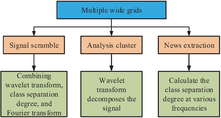
Figure 2 Difference evaluation method diagram of sub-signals at different frequencies.

Figure 2 shows the difference evaluation of multiple frequency pulse-coupled signal clusters. As shown in Figure 2, WT, CSD, and Fourier transform are first combined to interfere with the signal. Then, the signal is decomposed through WT. Finally, the CSD at different frequencies is calculated to evaluate the difference between sub-signals at different frequencies [17]. In this comparison process, the autocorrelation function of the sub signals is calculated to explore their correlation, as shown in Equation (5).

$$\{\begin{array}{c}\mathit{mod}(\rho ,l)=uuf+\{\rho ,l\}\hfill \\ \mathit{mod}(\sigma ,l)=uut+\{\sigma ,l\}\hfill \end{array}$$

(5)

In Equation (5), the mode of the pulse coupled sub signal is denoted as $\mathit{mod}()$. $\rho$ and $\sigma$ represent the signal coordinates at this moment, and their anti-interference ability is represented by $\mathit{uuf}$ and $\mathit{uut}$. $l$ represents the pulse width. Combining WT and CSD can provide a more comprehensive understanding of the characteristics of pulse-coupled signal clusters. During this process, WT can extract the time-frequency characteristics of the signal, while the role of CSD is to evaluate the separation of signal clusters. In addition, to better understand the characteristics of signals, the study provides CSD indicators for the signal analysis process, as shown in Equation (6).

$$\mathrm{\Delta }H=\sum _{i=1}^{LI}{\varsigma }_i\lg (2*{\varsigma }_i)$$

(6)

In Equation (6), the confusion in the signal analysis process is denoted as $\mathrm{\Delta }H$. The CSD indicator of the signal is represented by ${\varsigma }_i$. This method combines WT and CSD to analyze signal clusters, thereby comprehensively understanding signal feature information. Under the condition of improving signal processing and classification accuracy, the characteristic information of coupled signals with different frequencies is extracted for calculating CSD located in different environments, as shown in Figure 3.

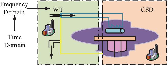
Figure 3 Feature information extraction of coupled signals at multiple frequencies.

As shown in Figure 3, the study first uses time-domain analysis to extract the peak amplitude and duration of the coupled signal, and then identifies specific features of the signal. Then, the frequency spectrum of the coupled signal is recorded using frequency domain methods to obtain the relationship between the frequency distribution and frequency components of the signal. In this process, wavelet analysis has the function of a time-frequency signal, which decomposes the signal into sub-signals of different frequencies and extracts the feature information of each sub-signal. The method follows Equation (7).

$$\{\begin{array}{c}{\omega }_{i,j}=\psi *{\varsigma }_i\hfill \\ {\xi }_{i,j}=\zeta *\mathrm{\Delta }H*E_X\hfill \end{array}$$

(7)

In Equation (7), $\omega$ and $\xi$ represent the pulse-coupled signal clusters of two frequencies, respectively. $\psi$ and $\zeta$ are the calculation process condition parameters for both. The instantaneous characteristic information of the coupled signal is recorded. The dynamic changes of the signal at different time points can also be identified, represented by $E_X$. In summary, this study combines the pulse coupled signal cluster feature analysis method (WTCSD) of WT and CSD, which not only helps to extract the time-frequency characteristics of the signal, but also evaluates the signal cluster separation, thereby providing more accurate results for radar radiation source signal analysis.

2.2 Wind Shear Feature Selection of Radar Radiation Source Signals

The above-mentioned WTCSD can extract the time-frequency characteristics of signals through wavelet transform and evaluate the degree of separation of signal clusters using class separation, providing a new perspective for feature extraction of radar signal sources. After delving into the feature extraction methods of radar signal sources, the next research will explore how to apply these features to wind shear prediction studies. WS is a complex meteorological phenomenon with diverse characteristics and rapid changes. In the feature selection of WS, the research focuses on several aspects such as wind speed and direction changes, spatial distribution, and duration. The change in wind speed is the main characteristic of WS, which can be manifested as rapid changes in a short period of time [18]. The magnitude of wind speed variation is taken as a characteristic indicator of WS, and monitored through the reflection intensity of radar radiation source signals. The method is shown in Figure 4.

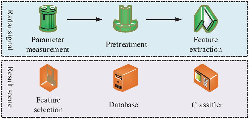
Figure 4 Monitoring method of reflection intensity of radar emitter signal.

Figure 4 shows the radar signal detection method. As shown in Figure 4, the study first installs radar sensors in the areas that need to be monitored to capture reflected signals. Based on the monitoring process of radar radiation sources transmitting signals, electromagnetic wave signals are sent to the target object. When the sensor receives the signal reflected back from the target object, the device can convert it into an electrical signal. This step can determine the strength of the reflected signal by processing the received signal. The reflection intensity is measured by calculating the power or amplitude of the signal, as shown in Equation (8).

$$\left[\begin{array}{c}\hfill {\chi }_{n+1}\hfill \\ \hfill {\epsilon }_{n+1}\hfill \end{array}\right]=\left[\begin{array}{cc}\hfill \iota \hfill & \hfill p\hfill \\ \hfill q\hfill & \hfill pq+\iota \hfill \end{array}\right]*\left[\begin{array}{c}\hfill {\chi }_n\hfill \\ \hfill {\epsilon }_n\hfill \end{array}\right]*{\mathit{mid}}_n$$

(8)

In Equation (8), the power and amplitude of the signal is denoted as ${\chi }_n$, and its reflection intensity is represented by ${\chi }_{n+1}$. The coordinates of the two are denoted as ${\epsilon }_n$ and ${\epsilon }_{n+1}$, respectively. $p$ and $q$ represent the change in wind direction during this process. ${\mathit{mid}}_n$ is the intermediate variable. This change manifests as a sudden reversal of wind direction, which has a significant impact on flight safety. Therefore, accurately monitoring wind direction changes can achieve WS feature selection. The spatial distribution is an important characteristic of wind direction variation, and there are significant differences in wind speed in space [19]. This study analyzes the spatial distribution of WS through the reflection intensity distribution of radar radiation source signals, as shown in Equation (9).

$$\mathit{KEY}=\{\sum _{i=1}^n{\mathit{key}}_i|n\in [1,64]\}$$

(9)

In Equation (9), the spatial difference in wind speed is denoted as $\mathit{KEY}$, where the WS feature is represented by ${\mathit{key}}_i$. When studying the duration, it manifests as the duration of continuous changes in wind speed. This study records the reflection intensity changes of radar radiation source signals over a period of time, and monitors the duration of WS. These WS feature selection contents are the basic features of WS. After analyzing and monitoring these features, the WS can be comprehensively understood, providing important basis for predicting WS of radar signal sources, as shown in Figure 5.

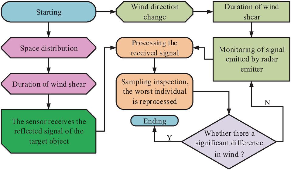
Figure 5 Wind shear prediction flow chart of radar signal source.

As shown in Figure 5, for existing meteorological radar equipment, this study obtains WS prediction of radar signal sources and calculates the reflection intensity of radar radiation source signals. After data preprocessing of radar radiation source signals, the quality and accuracy of the data are improved. Analyzing the reflection intensity of radar radiation source signals can screen the characteristic data of WS. In addition, the study selects the extracted WS features using correlation analysis, as shown in Equation (10).

$$B_{n+1}=u{B}_n*(1-B_n)$$

(10)

In Equation (10), $B_n$ represents randomly selected WS data, the WS of adjacent signal sources is denoted as $B_{n+1}$, and the radar connection between the two is denoted as $u$. The classification of radar radiation source signals is a key technology for identifying signal types. When the radar environment faces a wide variety of challenges, the modulation methods of existing signals are complex. This phenomenon can lead to frequent dynamic changes in parameters, making it difficult to effectively classify radar radiation source signals. To extract the phase information of the signal, Equation (11) is used.

$${\tau }_t(\mathrm{\ell },\mathrm{\Omega })={|{\xi }_0|}^{-0.5}*\tau (t{\xi }_0^{-t}-\mathrm{\Omega }{\upsilon }_0)$$

(11)

In Equation (11), the two forms of dynamic parameter changes are denoted as $\xi$ and $\upsilon$. $\mathrm{\ell }$, and $\mathrm{\Omega }$ represent the key technologies of radar signal recognition. $\tau$ is the conditional parameter of this process. The study records the measured reflection intensity data and uses a signal source acquisition method to display the variation of reflection intensity over time. Through these steps, the process of monitoring the reflection intensity of radar radiation source signals is achieved. Then, WS tracking and recognition operations are carried out, as shown in Equation (12).

$$F(t)=C*\sum _{-\mathrm{\infty }}^0\sum _0^{+\mathrm{\infty }}C(\mathrm{\ell },\mathrm{\Omega })*{\tau }_t(\mathrm{\ell },\mathrm{\Omega })$$

(12)

In Equation (12), the number of tracking and recognition operations for WS is denoted as $C$. Through this method, the periodicity and phase relationship of the signal can be obtained. The phase information of the signal can be extracted to obtain the phase characteristics and relationships of the coupled signal. In addition, the WS feature extraction of radar radiation source signals provide important technical support for WS prediction. In the construction of WS prediction model, the research is based on the WTCSDWS method, a WS feature extraction method related to radar radiation source signals is proposed based on the described WS feature selection content [20]. This method segments the obtained WS feature data into training and testing datasets using cross validation segmentation, as shown in Equation (13).

$$\{\begin{array}{c}{\kappa }_{i+1}=\nu {\lambda }_{\kappa }{\kappa }_i*(1-{\kappa }_i)+o{\mu }_i\hfill \\ {\mu }_{i+1}=\nu {\lambda }_{\mu }{\mu }_i*(1-{\mu }_i)+o{\kappa }_i\hfill \end{array}$$

(13)

In Equation (13), the initial situation of cross validation is denoted as $o$, and the training and testing datasets at time Y are represented by ${\kappa }_i$ and ${\mu }_i$, respectively. At this time, the WS features of them are denoted as ${\lambda }_{\kappa }$ and ${\lambda }_{\mu }$. ${\kappa }_{i+1}$ and ${\mu }_{i+1}$ represent the WS data measured by adjacent radar points. Then, feature selection is performed on the training dataset, and the most representative WS features are selected. This step utilizes correlation and principal component analysis, where the relationship between variables follows Equation (14).

$$v(Pt)=\sum _{i=1}^P\delta (x\to y)*C_i$$

(14)

In Equation (14), the number of parameter aggregations is represented by $Pt$. $C_i$ represents the vector value of wind direction. To validate the WS feature extraction method and construct the WS prediction model, experimental data is obtained from actual WS data collected by meteorological radar equipment, including spatial and temporal distribution characteristics. The relationship between them is shown in Equation (15).

$$\{\begin{array}{c}{T}_t(i,eg)={\chi }_{i\max }-v(t)\hfill \\ D_d(i,eg)={\epsilon }_{i\max }-v(P)\hfill \end{array}$$

(15)

In Equation (15), $eg$ represents the running time of the WTCSDWS model. $T_t$ and $D_d$ represent the distribution characteristics of WS time and location, respectively, and ${\chi }_{i\max }$ and ${\epsilon }_{i\max }$ are maximum values among them. In summary, the WS prediction model for radar radiation source signals provides vital technical support for WS prediction, and its specific performance needs to be experimentally verified.

3 Experimental Verification of WS Prediction Using WTCSDWS Based on WT

To verify the practical performance of the proposed WTCSDWS model in predicting WS in the radar signal clusters, the dataset used in the experiment is obtained from the weather radar of Tianfu International Airport. In this dataset, experiments are conducted on a total of 95 radars, each belonging to a different location. The evaluation indexes of the experiment in this study include energy loss, prediction range, prediction accuracy, etc.

3.1 Performance Analysis of WTCSDWS Model for Radar Signal Clusters

To make reasonable use of limited data, the data collected in the dataset from Tianfu International Airport is divided into two groups in a ratio of 8:12 to verify the learning performance and WS predictive performance of the model, respectively. A total of 6,144 pieces of data are used to test the learning performance of the model, and 9,216 pieces of data are used to test the WS prediction performance. Before the experiment, the equipment and parameters were determined for experimentation, as shown in Table 1.

Table 1 Equipment selection and parameter determination in the WTCSDWS model

Equipment Selection	Parameter Determination
System running memory	512MB
Data set	MREQ
Memory of graphics card	8T
Master client	Intel Zwoj A6-2022
Language	Easy Chinese
Number of radars	95
Operating system	Windows 11
Radar type	Long needle, shock absorber, leaky top, flawless type
Execution method	Matlab X52514l
System working time	15h,51min,23s
Terrain where radar is located	Coastal areas, deserts, ancient buildings, roofs

After determining the parameters for the experiment according to Table 1, the performance analysis experiment of the WTCSDWS model is conducted, and compared with the experimental results of the Random Forest (RF) model, WTC model, and SDWS model to verify the energy consumption of each model. The detailed information of the dataset is shown in Table 2.

Table 2 Detailed information of the dataset

		WS Event	Event to
Data Set	Sample Size	Sample Size	Non Event Ratio
Learning Performance Test Set	6144	1843	1:2.33
WS Prediction Performance Test Set	9216	2765	1:2.33
Total collection	15360	4608	1:2.33
Radar parameters	Radar antenna size	Radar radiation intensity	Radar scanning range
	30.48 cm	26–45 W/m	0–172 km

According to Table 2, the sample size of the dataset is 15360, and the sample sizes of the Learning Performance Test Set and WS Prediction Performance Test Set are 6144 and 9216, respectively. The event and non event scores are both 1:2.33. The experimental results are shown in Figure 6.

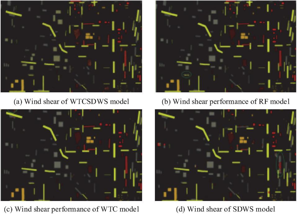
Figure 6 Experiment on the superiority of WTCSDWS model.

As shown in Figure 6, in the comparison of energy consumption among the four models, when the exploration area reached 652 hm${}^2$, the energy consumption of each model was 45 kW, 57 kW, 69 kW, and 81 kW, respectively. This indicated that the WTCSDWS model performed the best in terms of energy efficiency. As the radar coverage area expanded, the energy loss of the WTCSDWS model gradually stabilized. When the area increased to 896 hm${}^2$, the energy consumption of the model reached its optimal level, only at 65 kW, which was the lowest among all models, thus confirming the excellent energy-saving characteristics of the WTCSDWS model in WS prediction. As the radar coverage area increased, the power loss of the proposed model gradually stabilized. At an area of 896 hm${}^2$, it reached its optimal value of 65 kW. This value performed the best among the four models, indicating that it had the throttling characteristic in WS prediction. To verify the recommendation performance of the model in different environments, this study changes the external environment of the radar and conducts extensive experiments on the WS prediction ability of four models. The experimental results are shown in Figure 7.

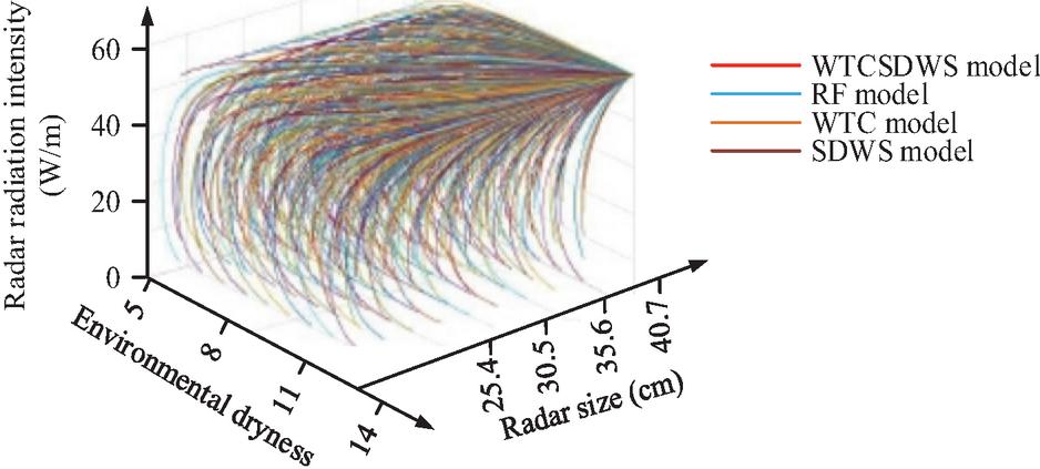
Figure 7 Extensive experiment of wind shear prediction ability of four models.

Figure 7 shows the extensive experimental results of the four models. In the proposed model, the radar radiation range was positively correlated with the dryness of the environment. As the radar signal increased, the coverage area of the radar decreased accordingly. When the radar size was 30.48 cm, the WS prediction ranges of the WTCSDWS, RF, WTC, and SDWS models were 45 W/m, 37 W/m, 32 W/m, and 26 W/m, respectively. The experimental performance of the WTCSDWS model was the best, indicating its strong stability. The accuracy of the WTCSDWS model is analyzed by calculating the WS of radar radiation sources under different conditions. The experimental results are shown in Figure 8.

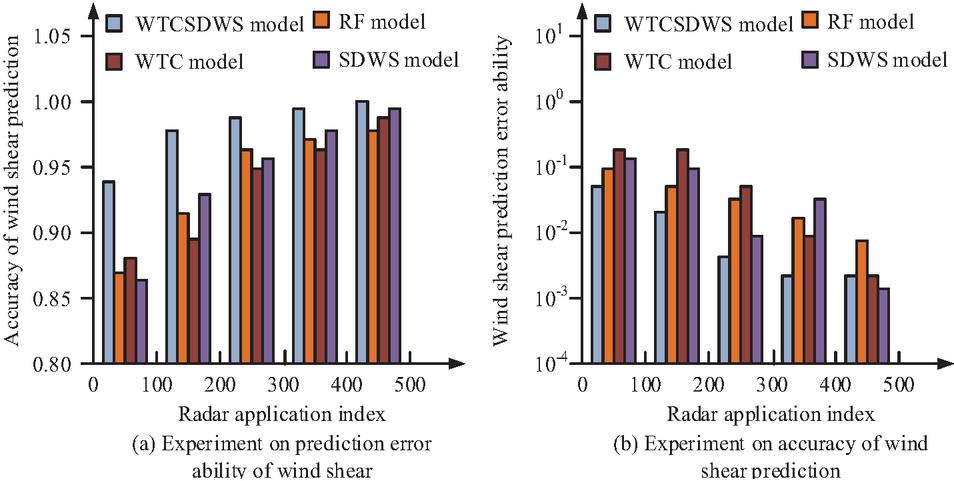
Figure 8 Accuracy test results of four models of wind shear.

As shown in Figure 8(a), as radar activity was increased, the accuracy of the four models in predicting WS correspondingly improved. When the radar activity was 375, their predictive effect on WS reached stability. At this point, the accuracy of the fusion model was the highest, at 0.98, indicating that the fusion model had the best WS prediction ability. As shown in Figure 8(b), all four models showed a decreasing trend in the WS prediction error. After the radar activity reached 400, their errors tended to stabilize. At this time, the errors of WTCSDWS, RF, WTC, and SDWS models were 3.5*10${}^{-3}$, 6.8*10${}^{-3}$, 21*10${}^{-3}$, and 45*10${}^{-3}$, respectively. The fusion model had the smallest error rate, indicating its best accuracy. The experimental results indicated that the model had superior performance. The study also conducts experimental verification for its effectiveness in WS prediction.

3.2 Verification of WS Prediction Performance Combining WT and CSD

To conduct WS prediction experiments of the WTCSDWS model in different radar signal sources in different regions, the study aims to control the radiation area of the radar to be the same and change the scanning time of the radar. Furthermore, the universality of the WS prediction is verified. The experimental results are shown in Figure 9.

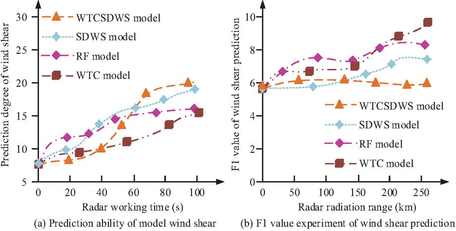
Figure 9 Extensive experimental results of wind shear prediction by WTCSDWS model.

Figure 9 shows the generalizability of the WTCSDWS model. As shown in Figure 9(a), the radar prediction level of all four models increased with the increase of radar working time. The highest radar prediction levels of WTCSDWS, RF, WTC, and SDWS models were 27, 16, 9, and 18, respectively, indicating that the fusion model had an advantage in cost-effectiveness. As shown in Figure 9(b), the F1 value (Harmonisal mean of precision and recall) of the WTCSDWS model was consistently the lowest among the four systems. When the radar radiation range was 172 km, its accuracy reached a stable level of 5.7. To conduct experiments on its robustness, the study conducts experiments, as shown in Figure 10.

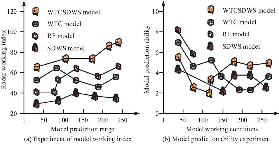
Figure 10 Robustness test of four models.

As shown in Figure 10(a), the WS prediction of the radar signal source by four models was directly proportional to the running time. The accuracy of the fusion model was 87.25%, which performed the best among the four models. As shown in Figure 10(b), the predictive ability of the four models varied with the increase of model running time, but the WTCSDWS model always performed the best among the four models. The experimental results showed that the proposed WTCSDWS model had accuracy, superiority, and robustness in predicting the WS of radar signal sources in radar signal clusters, which was suitable for improving radar monitoring capabilities. The long-term prediction results of different models’ Plan Position Indicator (PPI) scans are shown in Table 2.

Table 3 PPI scanning long-term prediction results

Model	Mean Value	Variance
WTCSDWS	0.958	0.017
WTC	1.234	0.235
RF	1.358	0.341
SDWS	1.169	0.153
Support Vector Regression	1.573	0.393
Neural network	1.423	0.231

According to Table 3, compared to other methods, WTCSDWS has smaller prediction mean and variance, which are 0.958 and 0.017, respectively, reducing by more than 18.0% and 88.9%, respectively. The above results indicate that WTCSDWS can achieve accurate prediction of wind shear. To verify the real-time performance and complexity of the proposed algorithm in practical applications, it was tested using measured data from Baiyun International Airport. The radar used at the airport is an S-band dual polarization phased array weather radar, with a working frequency of 2.885 G, antenna gain $\ge$44 dB, polarization mode of horizontal and vertical dual polarization, and a detection range of 460km. The real-time performance and complexity test results are shown in Table 4.

Table 4 Real time performance and complexity test results

	Single	Total Processing		Single Sample
	Signal	Time for 1000	Delay	Computational
	Inference	Consecutive	Stability	Capacity
Model	Delay (ms)	Samples (s)	(%)	(*10${}^6$ FLOPs)
WTCSDWS	85.6$\pm$ 4.2	89.8	4.9	86.3
RF	42.3 $\pm$ 3.1	45.5	7.3	23.5
WTC	58.7 $\pm$ 3.8	62.5	6.5	45.8
SDWS	63.2 $\pm$ 4.5	67.7	7.1	51.2

According to Table 4, compared to other algorithms, the proposed method has poor real-time performance and high complexity. This is because the multi-scale decomposition of wavelet transform requires a large amount of CPU computing resources, and parallel computing optimization is not currently used, resulting in a decrease in processing efficiency when signal frames are stacked.

4 Conclusion

With the continuous development of WS prediction models, the working goal of the model gradually tends to refine flying objects. To enhance the predictive ability of radar signal sources in the radar signal cluster, this study combined WT and CSD to apply WTCSDWS in WS prediction. To verify the superiority of the model, the experimental results of the other three models were compared. When the exploration area was 652 hm${}^2$, the energy consumption of the WTCSDWS, RF, WTC, and SDWS models was 45 kW, 57 kW, 69 kW, and 81 kW, respectively, indicating that the WTCSDWS model had throttling ability. When the radar was 30.48 cm in size, the ranges of WTCSDWS, RF, WTC, and SDWS models were 45 W/m, 37 W/m, 32 W/m, and 26 W/m, respectively. The experimental results showed that the proposed WTCSDWS model had effectiveness, universality, and robustness in predicting the WS of radar signal sources, which was suitable for improving the flying object monitoring capability of radar signal clusters. However, due to the integration of WT and CSD into the fusion model, the complexity of the model has increased, resulting in high computational costs and long processing time, which limits the fast response performance of the model. Meanwhile, due to the fact that the model is aimed at the civil aviation field, its scalability is poor, which is only applicable to climate radar systems at airports. Therefore, in the future, we will consider establishing a “standardized interface for radar signals” and designing adaptive preprocessing modules for different types of radar output parameters (such as frequency bands, scanning frequencies, and signal amplitude ranges) to achieve compatibility between the model and civilian airport radars, military meteorological radars, and small portable radars, thereby enhancing the ability for large-scale deployment.

References

[1] Ning Y, Zhang Y, Li X. “Towards accurate coronary artery calcium segmentation with multi-scale attention mechanism”, IET Image Processing, 2021, 15(6): 1359–1370.

[2] Zhang H, Shen X. “A dynamic tooth wear prediction model for reflecting “two-sides” coupling relation between tooth wear accumulation and load sharing behavior in compound planetary gear set”, Proceedings of the Institution of Mechanical Engineers, Part C: Journal of Mechanical Engineering Science, 2020, 234(9): 1746–1763.

[3] Nsugbe E. “Toward a Self-Supervised Architecture for Semen Quality Prediction Using Environmental and Lifestyle Factors”, Artificial Intelligence and Applications, 2023, 1(1): 35–42.

[4] Mo S, Yue Z, Feng Z. “Analytical investigation on load-sharing characteristics for multi-power face gear split flow system”, Proceedings of the Institution of Mechanical Engineers, Part C: Journal of Mechanical Engineering Science, 2020, 234(2): 676–692.

[5] Yumatov E A, Dudnik E N, Glazachev O S, AI Filipchenko, SS Pertsov. “Revealing True and False Brain States Based on Wavelet Analysis of Electroencephalogram”, Neuroscience and Medicine, 2022, 13(2): 61–69.

[6] Gowthami V, Bagan K B, Pushpa S E P. “A novel approach towards high-performance image compression using multilevel wavelet transformation for heterogeneous datasets”, The Journal of Supercomputing, 2023, 79(3): 2488–2518.

[7] Singh A K, Saxena A, Roy N. “Inter-turn fault stability enrichment and diagnostic analysis of power system network using wavelet transformation-based sample data control and fuzzy logic controller”, Transactions of the Institute of Measurement and Control, 2021, 43(12): 2788–2798.

[8] Sun M, Wang H, Liu P. “Stack autoencoder transfer learning algorithm for bearing fault diagnosis based on class separation and domain fusion”, IEEE Transactions on Industrial Electronics, 2021, 69(3): 3047–3058.

[9] Chui C K, Jiang Q, Li L. “Signal separation based on adaptive continuous wavelet-like transform and analysis”, Applied and computational harmonic analysis, 2021, 53(7): 151–179.

[10] Koldovský Z, Kautský V, Tichavský P. “Dynamic independent component/vector analysis: Time-variant linear mixtures separable by time-invariant beamformers”, IEEE Transactions on Signal Processing, 2021, 69(8): 2158–2173.

[11] Zafar A, Aamir M, Nawi N M. “An Optimization Approach for Convolutional Neural Network Using Non-Dominated Sorted Genetic Algorithm-II”, Computers, Materials & Continua, 2023, 74(3): 5641–5661.

[12] Charles D. “The Lead-Lag Relationship Between International Food Prices, Freight Rates, and Trinidad and Tobago’s Food Inflation: A Support Vector Regression Analysis”, Green and Low-Carbon Economy, 2023, 1(2): 94–103.

[13] Hou L, Lei Y, Fu Y, Hu J. “Effects of lightweight gear blank on noise, vibration and harshness for electric drive system in electric vehicles”, Proceedings of the Institution of Mechanical Engineers, Part K: Journal of Multi-Body Dynamics, 2020, 234(3): 447–464.

[14] Yangbing Z, Xiao X, Xing W, Mingyue C, & Lu C. “Stability Modeling and Analysis of Grid Connected Doubly Fed Wind Energy Generation Based on Small Signal Model”. Distributed Generation & Alternative Energy Journal, 2023.

[15] Song Y, Mo S, Feng Z, Song W. “Research on dynamic load sharing characteristics of double input face gear split-parallel transmission system”, Proceedings of the Institution of Mechanical Engineers, Part C: Journal of Mechanical Engineering Science, 2022, 236(5): 2185–2202.

[16] Ballaji A, Dash R. “A Comprehensive Review on Latest State of the Art Practices in MPPT Algorithm”. Distributed Generation & Alternative Energy Journal, 2023.

[17] Liu Y, Li Y, Ma L. “Parametric design approach on high-order and multi-segment modified elliptical helical gears based on virtual gear share”, Proceedings of the Institution of Mechanical Engineers, Part C: Journal of Mechanical Engineering Science, 2022, 236(9): 4599–4609.

[18] Reddy B, Reddy V, Kumar M. “Design and Analysis of DC-DC Converters with Artificial Intelligence Based MPPT Approaches for Grid Tied Hybrid PV-PEMFC System”. Distributed Generation & Alternative Energy Journal, 2023.

[19] Amin S N, Shivakumara P, Jun T X, Chong L, Zan D L L, Rahavendra R. “An Augmented Reality-Based Approach for Designing Interactive Food Menu of Restaurant Using Android”, Artificial Intelligence and Applications, 2023, 1(1): 26–34.

[20] Wang Y, Luo Y, Ren J. “Research on application of spatial attention mechanism in the super-resolution reconstruction of single-channel greyscale image of mouse brain”, International Journal of Wireless and Mobile Computing, 2022, 22(3–4): 259–264.

Biographies

Ting Xu obtained her master’s degree in Meteorology (2014) from Institution of Atmospheric Physics, Chinese Academy of Sciences. She is working as an Associate Professor in the Department of Aviation Meteorology, College of Aviation Meteorology, Civil Aviation Flight University of China. Her areas of interest include aviation turbulence and low-level wind shear.

Qionghua Li obtained her bachelor’s degree in Atmospheric Sciences (2011) from College of Atmospheric Sciences, Lanzhou University. She currently serves as the Chief Engineer at the Meteorological Station of Jiangxi Air Traffic Management Sub-Bureau, East China Regional Administration of Civil Aviation of China, specializing in weather forecasting and observation work.

Yan Lu obtained her bachelor’s degree in Atmospheric Sciences (2011) from College of Atmospheric Sciences, Lanzhou University. She is working as a Meteorological Business Manager in Heilongjiang Airport Management Group Co., Ltd, responsible for providing guidance, supervision, and inspection of meteorological operations at the regional airports in Heilongjiang Province. Her areas of interest include studying the impact of complex weather on airport operations and flight.

Distributed Generation & Alternative Energy Journal, Vol. 40_5&6, 1281–1304.
doi: 10.13052/dgaej2156-3306.405615
© 2025 River Publishers