Enhancing Intelligent Fault Detection and Classification in Power Grid Engineering Using LSTM Neural Networks
Qinghua Chen*, Tao Xu, Cheng Zhou and Yating Wang
State Grid Jiangxi Economic Research Institute, Nanchang, 330006, China
E-mail: tsingva@126.com; tao_xu01@outlook.com; cheng_zhou01@outlook.com; yating_wang001@outlook.com
*Corresponding Author
Received 20 September 2025; Accepted 25 April 2026
Abstract
Power grid engineering is necessary for the distribution of power, but problem detection and categorization are made extremely difficult by their growing complexity, particularly with the incorporation of renewable energy sources. Decision trees and support vector machines are two examples of fault detection techniques that frequently fail to handle the dynamic and non-stationary character of power grid data. These techniques’ efficacy in real-time defect identification is limited because they are unable to capture the complex relationships and temporal dependencies present in time-series data. Furthermore, a lot of conventional models are unable to generalize to different kinds of problems, which results in errors and delays in fault identification. For improved fault detection and classification in power grids, this research suggests a hybrid approach that combines Temporal Fusion Transformers (TFT) with Long Short-Term Memory (LSTM) Neural networks. While the LSTM neural network is used to represent sequential data, the TFT model is particularly good at capturing complicated linkages in time-series data. By combining these two models, the suggested approach can improve grid efficiency and dependability by offering precise fault forecasts in real-time. The findings show that the suggested hybrid model works better than conventional techniques, with a fault classification accuracy of 98.66% as opposed to decision trees’ 97.42% and SE-CDAE’s 97.98% accuracy. The performance of the model demonstrates its potential for real-time implementation in contemporary power grids, guaranteeing improved fault identification and prompt reactions to avert system breakdowns.
Keywords: Fault detection, power grids, temporal fusion transformers, long short-term memory, renewable energy.
1 Introduction
The combination of renewable sources of energy, such as wind and solar, and the increasing complexity of power grids presents new challenges when attempting to detect and predict faults. Power grids are critical in the distribution of electricity sources to end users [1]. In the past, fault detection has relied on a threshold to select nominal values and simple algorithms, which have struggled to communicate with more modern and dynamic (and complicated) systems [2, 3]. Because of the unpredictable and intermittent nature of renewable sources of energy, output levels can fluctuate, which may require making rapid adjustments to maintain stability, and not providing end-users with the reliability of supply that they expect. The need for increased response times and adjustments will continue as power grids grow larger, have more decentralized resources, and technically-motivated smart grid technology. For many power systems, operationally complex and evolving with purpose may entail disruptions to their operation [4, 5]. Rehabilitation of this reliability, capacity, and operational efficiency are piecemeal efforts should a fault occur. This variability also translates into a large volume of real time data and therefore methods must be fit for purpose to integrate renewables without affecting the reliability.
One of the major difficulties in detecting faults in power grid systems is their unpredictability and volatility. Faults can occur for many reasons, including equipment failure, changing environmental factors, and human error, all of which complicate the sourcing and analysis of the data for the grid system [6, 7]. Faults behave in ways that are both highly dynamic and often non-stationary, even making them non-stationary in nature, which makes it difficult to capture the data using established fault detection methods and static models or thresholds. Smart grid technology has added technology advanced sensors, IoT devices and real time data collection capabilities, leading to an information overload where data is valuable but overwhelming, adding more complexity and challenges [8, 9]. Smart grid technology is always producing data so the key challenges of IoT based systems is learning how to process, store and analyze every stream of data in real time. The common fault detection methods will typically not work with the scale of data because of the volume and complexity of operational data generated, which can magnify the lapse time for fault detection, prolong grid downtime and/or cause operational inefficiencies [10]. The lack of agile response and analysis for such a large dynamically changeable dataset is an emerging weakness in fault detection systems but it is also an opportunity to develop data mining approaches to data-driven modern fault detection systems.
Although there has been considerable advancement in the fields of ML and data analytics, the state of the art of fault detection and prediction about power grids remains severely limited by numerous challenges that keep it from being effective or useful in real-world applications [11, 12]. Most approaches are based on past data or experience without taking into account the temporal dependency of power system behavior, making them not robust to the highly dynamic operational environment of the grid. Also, traditional machine learning algorithms, such as decision tree and support vector machine classifiers, were designed to operate mainly on vector data; however, many power systems unavoidably create large amounts of high-dimensional, streaming, sequential data [13]. Moreover, model-based fault detection algorithms have generally suffered shortcomings in their generalization performance for new, unseen fault types, and they can only be used in highly controlled situations where the exact circumstances and features of the fault are properly controlled in the model. Further complicating the situation, including differences between faults in regards to severity, duration, and the location of the faults, so known faults generally do not lend themselves to prediction [14, 15]. Furthermore, the issue of proactively predicting faults to allow for timely action is problematic in systems with time-variable loads, or systems which incorporate high levels of renewable energy. Ultimately, contemporary fault detection and prediction methods are limited in their ability to handle the complex operations and contingencies of modern power grids, which emphasizes the need for more advanced, adaptive, and accurate fault detection and prediction methods that can handle a vast amount of real data.
The proposed method presents a hybrid model that combines TFT and LSTM neural networks to improve power grid fault detection and classification tasks. The new method is able to utilize the power of TFTs to leverage limited capabilities to understand long-range temporal dependencies and complex relationships in time-series datasets, where LSTMs are more efficient in modeling sequential data and quantifying short- and long-term characteristics. By combining two models, the proposed method is capable of summarizing real-time data from the power grid, logging both voltage and current, and potentially frequency in a power grid to combine the possible outputs of each fault state (“Normal,” “Faulty,” and “Overheated”). The hybrid model allows for interpreting challenges from the dynamism and non-stationary nature of power grids while improving the ability to have more reliable detection and enhance operating efficiency, especially for modern power systems utilizing renewable energy sources.
Key Contributions
• Developed a hybrid model combining TFT-LSTM neural networks to enhance fault detection and classification in power grids.
• Addressed the limitations of existing fault detection methods by effectively evaluating their performance.
• Achieved superior performance compared to traditional machine learning models, with an accuracy of 98.66%, demonstrating the robustness of the proposed method in handling complex fault patterns.
• Provided a reliable framework for fault detection, minimizing FP and FN, and improving the operational efficiency of modern power grids integrating renewable energy sources.
• The article is structured with related works in Section 2 and problem statement in Section 3. Section 4 discusses the suggested technique, and Section 5 presents the findings. The essay is concluded at Section 6.
2 Related Works
Almasoudi [16] looks into how AI can be embedded into modern power generation grids specifically within the framework of the 4IR, thus enhancing detection and prediction.. Yet, the complexity of the real-time data analysis and guaranteeing precision and effectiveness in large grid structures limit these approaches. Najafzadeh et al. [17] developed new technologies in ML techniques is a way to improve smart grid surveillance and fault detection. It predicts abnormalities in a transmission line in rapid prediction through fuzzy thresholding based on line voltage. It uses DT and RF methods developed by wild horse meta-heuristic methods to derive value frequencies for fault characterization. An artificial system with fuzzy inference is adjusted by the current results to accurately identify errors in real-time power transfer systems score.
Hosamo et al. [18] propose a Digital Twin proactive maintenance system for AHUs as part of the effort to tackle deficiencies in the current structural management systems adopted into practice. The aforementioned system implements three modules: fault diagnoses based on the APAR method, condition forecasting based on, and maintenance planning of BIM, IoT, and semantic computational approaches for more effective maintenance techniques. The technical viability and practical utility of the proposed methodology for predictive servicing to AHUs are validated by a real case study for an educational institution in Norway. Shakiba et al. [19] propose a trustworthy methodology for the identification and detection of high-voltage transmission line faults using CNNs, which can enhance the precision and speed of fault recovery. The methodology is to be examined under variations of phasing differentiation, fault obstruction, source inductive voltage, fault initiation angle, changes in bus voltage, and measuring noise with a view to establishing the robustness of the approach in uncertain and chaotic environments. Although the method depends on the accuracy of the input data and on how fast drastic system parameter changes can be managed before disconnections, the evaluation was also made for the delay.
An ensemble approach has been proposed by Zhang [20] for continuous fault detection on a single-phase PWM rectifying system with the signal prediction on NARX and ELM to provide improved prediction accuracy and robustness to the system. Faults are detected by developing a residual based on the difference between the prediction and the sensor outputs, and then comparing it with the fault threshold to classify those faults according to complaints and residue assessment. However, despite being an effective method, this one is constrained due to its dependency on the quality of historical data and the system’s capability to handle changing load variations during operation. Sridharan and Sugumaran [21] present an automated fault diagnostic measurement using PVM based on CNN for classifying the different problems using photographs made with UAVs. Data augmentation is applied to existing aerial photographs to remove the restrictions caused by the dataset. The images are then used by the CNN model for feature extraction and classification. The shortcoming of this technique is that it relies on an adequate number of good-quality labeled pictures; this affects the model’s performance but increases the model’s effectiveness in fault identification due to the image quality and variation in the supplemented dataset.
To account for the non-steady nature of wind power messages, Ding et al. [22] proposed hybrid short-term wind power forecasting algorithm combines the WOA, the CEEMD method, and KELM. In this algorithm, the wind power forecast is obtained from an optimal KELM model performed through WOA, decomposition of unsteady wind power data set into stationary components using CEEMD, and finally superimposing their forecasts. One limitation of this technique is that the entire forecast accuracy may be affected due to errors in these processes. Thus, it heavily depends on the quality of optimization and decomposition methods. Mostafa, Ramadan, and Elfarouk [23] discusses the use of big data in analyzing the smart grid and renewable power plants and proposes five steps for predicting the reliability of a smart grid using various techniques. For the prediction of reliability in case of distributed smart grid architecture, different ML models are studied. Again, future research should focus on using a larger dataset with broader sources of renewable energies over various sites since the rather small dataset used in the present study may affect the generalization of conclusions.
Chen, Wang, and Zhang [24] employs SVM, NN, and RF in the online condition monitoring, detection, and diagnosis of brushless motor defects and, further, develops an ML-based technique for detection and diagnosis of faults in brushless motors. The whole research aims to find out the various types of defects, understand the effects on severity, and develop efficient remedies. However, the dependence of such a procedure on the quality of sensor data is a major point in which the precision of the model can be compromised. Zeng et al. [25] proposes a novel advanced form of the ABFPN; an advanced multiscale feature fusion scheme designed for the efficient extraction of small objects through the integrated atrous Fourier operations and skip connections. Such features are said to be integrated into an improved PCB defect identification structural model called IPDD, which presents a number of strong algorithms for enhancing detection performance on small surface defects on PCBs. Nevertheless, the main limitation of this method arises from its high dependence on properly annotated datasets and expensive computation engines, thus limiting the applicability of the approach to other defect identification scenarios.
The remaining connections capable of solving the gradient vanishing problem then lead Khan et al. [26] to propose a competent ESNCNN forecasting scheme for RE, which uses CNN for spatial data and ESN for nonlinear connection modelling. Its increased prediction accuracy, which takes temporal complexities into account, shows a more reliable approach to integrating RE in smart power systems. A drawback of this method is its reliance on well-diverse datasets for training, which may lead to varying functional efficiency depending on generalization to other energy sources. Using ML methods alongside sampling techniques, such as artificial minority oversampling and Tomek’s linking, for fault data that are decidedly unbalanced in the electricity monitoring of machines is the principal focus of this research. Swana, Doorsamy, and Bokoro [27] compares various techniques for diagnosing faults in induction machines with wound rotors and discusses problems arising mainly due to imbalanced data sets and the scarcity of trustworthy labeled fault data. The disadvantages of an approach that relies heavily on artificially creating data are that sometimes these simulations may not adequately represent real-world fault events. Furthermore, model performance varies with the nature of data creation.
2.1 Problem Statement
• Conventional methods of fault detection in power grids can fail to maintain the timeliness and accuracy of locating faults, leading to extended downtimes and high operational costs. These methods, may struggle to deal with the complexities of the real-time data with which they must work, especially in relation to nonlinear and non-stationary fault patterns [28].
• Existing power grid fault prediction models in ML generally aim towards improving their accuracy while lacking in terms of time complexity and real-time attainment of their fault detection potential. Such a scenario means that the models may never generalize well for different types and conditions of faults that characterize dynamic grid environments [29].
• Power grid faults develop from convoluted and long-term behavior and interactions associated with system dynamics being modelled poorly by simple neural and decision trees. Most contemporary techniques fail to exploit temporal dependencies present in grid data, hampering efficient prediction of faults before their serious adverse effects occur [30].
• Present fault detection and prediction techniques are quite rigid in their application, especially since smart grids require responses that can adapt to dynamic and real-time conditions. Thus, the ineffectiveness of transforming solutions to these current real-data data and distributed networks is due to poor integration of existing techniques [31].
To address these limitations, the proposed approach is a hybrid of TFT-STM networks, which help accurately identify and classify faults in power grids.
Objectives
• Develop a hybrid model combining TFT-LSTM neural networks to enhance fault detection and classification in power grids.
• Address the limitations of existing fault detection methods by effectively evaluating their performance.
• Achieve superior performance compared to traditional ML models, aiming for higher accuracy, to demonstrate the robustness of the proposed method in handling complex fault patterns.
• Provide a reliable framework for fault detection and improving the operational efficiency of modern power grids, integrating renewable energy sources.
3 Proposed TFT-LSTM Framework
The process of identifying and classifying power system faults is depicted in Figure 1. The first step in this process is to collect data, and in this case, power system fault data, which is then transformed. The processes include the steps of resampling, label encoding, and min-max scaling, to provide the data for the next step. After pre-processing, the next phase is the detection and classification of faults through the TFT-LSTM model type, where the model can classify three categories of faults as ‘Normal’, ‘Faulty’, and ‘Overheated.’ When completed, the models are measured against a standard. Finally, the model is optimized using the SHO method. All these processes enable a robust framework for effectively detecting and classifying faults in power systems.
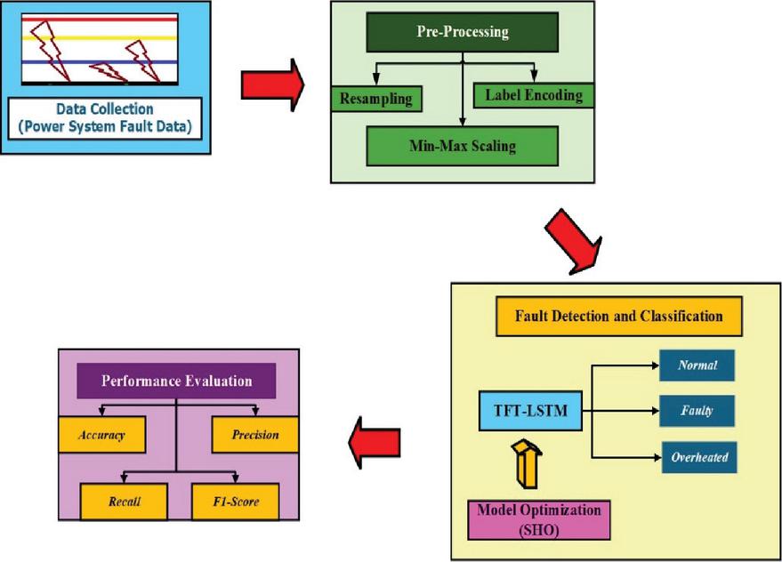
Figure 1 Proposed TFT-LSTM framework.
3.1 Data Collection
The dataset employed in this study is the “Power System Faults Dataset” available on Kaggle (Ziya07, Version 1.0), accessed on 8 May 2025. The dataset contains labeled time-series measurements of voltage, current, load, and temperature variables. An 80%–20% stratified train–test split was applied to preserve class distribution and prevent data leakage. Explicit reporting of dataset version and access date ensures reproducibility and experimental transparency. The Dataset for Power System Faults from Kaggle is rich and comprehensive in terms of data on power system faults, essential in attempting to construct or test models for detecting and predicting faults. The dataset portrays several fault types along with the system exposure parameters: voltage, current, and power readings that are crucial for studying the behavior of a power system under given fault conditions. Using this dataset, intrapreneurs and researchers can train ML algorithms to classify types of faults and thus predict their occurrence while balancing with system reliability. Being a dataset available on Kaggle, it can be accessed by a wide range of consumers to advance more efficient and accurate fault detection methodologies in power grid systems [32].
The dataset represents offline historical recordings collected under controlled and simulated operational conditions rather than live streaming sensor measurements. The time-series observations were generated to reflect realistic electrical behavior across normal, faulty, and thermal stress scenarios. Although the data were not acquired in real time, the sequential structure preserves temporal continuity required for dynamic modeling. The sampling format closely resembles practical monitoring intervals used in grid systems. This structure enables realistic simulation of deployment conditions in intelligent fault monitoring environments.
3.2 Pre-Processing
The Pre-Processing stage is when the dataset is prepped to help machine learning models, via cleaning, transforming, and preparing data. This involves dealing with missing values, removing outliers or treatment of outliers, and scaling out features to make data near equivalent (example, Min-Max Scaling would be the method it uses to normalize data across features.). It also takes care to make categorical variables equivalent numerical values creating label encoders and it also can use resampling methods to tackle class imbalances to create balanced datasets to help train the dataset better.
3.2.1 Min-Max scaling
Min-Max scaling is an important step in normalizing the features in the Power System Faults Dataset to a common scale, typically ranging from 0 to 1, and is essential for obtaining optimal performance from machine learning models. Power systems data usually contains features that vary in units and magnitudes, for example, current, voltage, and frequency, which means there will be a significant difference in the numerical values when compared to each other. Without normalization, the larger numerical values would influence the model’s training process in a disproportionate manner and could lead to biased predictions or worse convergence. Min-Max scaling make sure that all inputs are processed as equals. Min-max scaling can represent these features on some common scale, so no feature is favoured over another. The goal of preprocessing is to improve the interaction with the algorithm, and min-max scaling facilitates a more efficient structure for convergence and helps algorithms to run more efficiently. As far as transforming features, it can be mathematically defined with Equation (1):
| (1) |
Where: X is the original value, is the scaled value.
3.2.2 Label encoding
The Power System Faults Dataset used Label Encoding to translate categorical variables, such as fault types (such as “Normal”, “Faulty”, and “Overheated”) into numeric values for machine learning models to be able to consume them. Most ML algorithms require the input features to be in a numerical format, including decision trees and neural networks. Label Encoding assigns a separate numeric value to each categorical variable, transforming categorical labels into numerical values for use in training the model. For instance, “Normal” could be assigned an encoding value of (0), “Faulty” could be assigned an encoding value of (1), and “Overheated” could be assigned an encoding value of (2). This is significant since these categories allow the model to distinguish between the fault types as group classifications and classify the state of the system accurately. Label Encoding can also be expressed mathematically in Equation (2):
| (2) |
Where: X is the original categorical feature, y is the transformed numerical representation.
3.2.3 Resampling
Within the Power System Faults Dataset, resampling is quite important to address the issue of class imbalance. Class imbalance occurs when one or more of the fault types have very few examples compared to the fault types that have many, such as “Faulty” when compared to “Normal” type faults. The extent of class imbalance will have a direct impact on how an ML model can be accurately and generally trained, because in the case of serious class imbalance, the algorithms can potentially exploit these majority classifications by justly predicting majority cases and negating the minority classes, which could result in very poor detection and classifications of fault types with very few examples. Resampling techniques will allow either oversampling the minority classification by producing or generating new synthetic extra samples for this class, or undersampling the majority by removing or downsampling their total examples. Both methods will allow a more balanced distribution of fault type categories and will provide the model with an accurate and representative dataset where it can learn from the many cases and the few cases, allowing it to learn the features of each fault type. This balanced dataset will allow it to detect fault signs and permit accurate and robust classifications of faults of both majority and minority types, so the power grid monitoring fault detection system will be as reliable as possible. It is given in Equation (3).
| (3) |
Where: X represents the original dataset, represents the resampled dataset.
The operational states were defined using standard electrical threshold criteria. The Normal class corresponds to voltage and current values within 5% of nominal ratings under stable temperature conditions. The Faulty class reflects deviations exceeding 10% in electrical parameters, indicating abnormal disturbances. The Overheated class is characterized by temperature values exceeding safe operational limits (above 80–90∘C), indicating thermal stress conditions.
3.3 Fault Detection and Classification Using TFT-LSTM
In this section, Using TFT-LSTM, it used the TFT model and LSTM neural networks are used as separate models to process time series input sent from the power grid, and make any predictive estimations based on any fault detections possible. The TFT model captures long-range temporal dependency and complex interrelationships among the input, while the LSTM model takes a sequential path to process the input. The outputs from the models will be used to classify the system state into actionable fault classifications (“Normal”, “Faulty”, and “Overheated”) and to provide real-time fault detection and classification capabilities to the system operator. The hybridized solutions will provide improved identification of faults to enable grid operators to react and take corrective action and to maintain a stable and efficient power grid.
The Temporal Fusion Transformer was configured with 4 multi-head attention heads to effectively capture diverse temporal dependencies across input sequences. The hidden layer dimension was set to 128 units, while the embedding dimension was fixed at 64 to ensure compact yet expressive feature representation. A dropout rate of 0.2 was incorporated to mitigate overfitting and enhance generalization capability. Model training was conducted using the Adam optimizer with a learning rate of 0.001 to ensure stable convergence. These hyperparameter settings support efficient temporal attention learning and robust feature fusion within the hybrid framework.
3.3.1 Input data representation
In the Input Data Representation stage of this article, the power system fault data is organized into a time-series format so that each data point has a specific time stamp, containing system parameters such as voltage, current, and frequency. The fault data is separated into input features and target labels, where the input features used include historical measurements of the system, and the target labels have reference to the fault type (for example, “Normal,” “Faulty,” or “Overheated”). The normalized input features were pre-processed using Min-Max Scaling and Label Encoding to ensure they are ready for model training, and meaningful information could be provided to the TFT-LSTM hybrid model for fault detection and prediction. It is given in Equation (4).
| (4) |
A temporal window size of 20-time steps was selected to balance short-term fluctuation detection and long-range dependency modeling. Smaller windows failed to capture gradual fault evolution, whereas larger windows increased computational complexity without significant accuracy improvement. Empirical evaluation demonstrated stable convergence and improved classification performance at this length. The chosen window ensures efficient sequential dependency learning.
3.3.2 Temporal fusion transformer
In this stage, the TFT serves as a dedicated model for time-series data for both fault detection and fault prediction. Designed with a combination of attention mechanisms and GRNs that can capture higher-order temporal dependencies and learn useful features based on both dynamic and static inputs. The model will ingest historic data through GRNs, activate attention mechanisms to learn long-range dependencies, and provide a model format that jointly considers both temporal (dynamic and static) and state representations. The processed representation will then proceed to a prediction layer that will return the class of the system state (for example, “Normal”, “Faulty”, “Overheated”), and allows component predictions of real-time fault detection and prediction. This develops both a correlation to handle non-linear and dynamic tracing of power grid time-series data, while providing robust and timely predictions.
3.3.3 Gated residual networks (GRN)
In the scope of this paper, the GRN is used within the TFT model to achieve the capability of the time-series input data from the power system. The GRNs take the time-series input features (voltage, current, frequency), and learn complex relationships via residual connections, which help prevent vanishing gradient problems and allow more effective learning. By employing gating mechanisms, the model can consider temporal dynamics and fluctuations of the power grid data to improve overall fault detection and prediction performance. It is given in Equation (5).
| (5) |
Where: is the hidden state, is the input, s the weight matrix, b is the bias term.
3.3.4 Attention mechanism
The Attention Mechanism of the TFT model can help the model to focus on the most useful parts of the time-series data when predicting faults within the electrical grid. The model provides an attention score to the different time steps in the time-series data, thus portraying the importance of various past observations (ten significant time steps back in the past) about not only the voltage, current, or frequency but also when there are significant changes regarding a possible fault status. While the model has emphasized these past observations (time steps) with an attention score, it is only to facilitate the model to pick up the more important patterns in the time-series data, which is required for optimal fault detection and prediction. It is given in Equation (6).
| (6) |
Where: is the query vector, is the key vector.
3.3.5 Prediction layer
The Prediction Layer in the TFT model described in this paper was explored in detail in the previous section. The Prediction Layer uses the contextualized processed features from previous layers that contain both dynamic and static inputs to generate the final output prediction. The Prediction Layer uses the output of the attention and gated residual networks to predict the fault class or system state (e.g., “Normal”, “Faulty”, or “Overheated”) at each time step. The prediction layer usually makes its predictions with an FC layer, meaning that all temporal and feature interactions learned have been aggregated, allowing the model to output a probability distribution across the fault classes, making accurate fault type detection and classification possible. It is given in Equation (7).
| (7) |
Where: represents the predicted output.
3.4 Long Short-Term Memory
In this step, model and predict time-series dependencies in the sequential data stream from the power grid data, use of a LSTM neural network. LSTMs also have gates forget, input, output gates that allow the model to remember, update, or forget past data, reducing noise from less informative features of the time-series sequential data and concentrating on the most relevant features to fault detection. The LSTM in can incorporate time-series data from time steps in the past to use the sequential dependencies to predict whenever a fault will occur or apply any changes that increase fault detection or prediction performance in real time and dynamic operation of the grid system. The LSTM component is structured using two stacked recurrent layers to enhance hierarchical temporal representation learning. Each layer contains 128 hidden units to ensure sufficient memory capacity for modeling sequential dependencies. A dropout rate of 0.2 is applied between layers to reduce overfitting and improve generalization stability. The stacked configuration enables progressive refinement of contextual embeddings generated by the preceding TFT module. This architectural design balances depth, representational power, and computational efficiency within the hybrid framework.
3.4.1 Forget gate
The Forget Gate in LSTM neural networks is the one that determines what information from the previous time step should be forgotten from the memory cell. This gate is typically meant to forget information that is no longer relevant or out-of-date to the memory cell itself, allowing the model not to be fooled or misled by the previous time step. The Forget Gate allows the LSTM to remember a time frame, and when that time frame becomes irrelevant (newer information or time step), the Forget Gate is key for fault prediction and classification, specifically for our power grid system. It is given in Equation (8).
| (8) |
Where: is the forget gate.
3.4.2 Input gate
The Input Gate makes decisions about what input information moves from the input layer to the memory cell of the LSTM neural network. The input gate is a gate used to assist the model in storing relevant facets of the new data and updating memory features, such as changes in voltage or current, when detecting and predicting faults within power grid systems. It is given in Equation (9).
| (9) |
Where: this is the input gate.
3.4.3 Cell state update
The Cell State Update in the LSTM neural network updates the memory cell according to the values from the Input Gate and the previous cell state. This allows the model to preserve long-identified dependencies and update cell state with appreciable segments of information (i.e., values of power grid parameters changed appreciably) so that even past important indications might influence future fault prediction and classification decisions. It is given in Equations (10) and (11).
| (10) | ||
| (11) |
Where: is the candidate cell state, is the cell state.
3.4.4 Output gate
The Output Gate in the LSTM neural network investigates the updated cell state after the forget and input gates, to determine what portion of the new cell state is the output model’s prediction at a specific timestep. The output gate is then used to evaluate how much information about the updated cell state is applicable to transmit to the following layer of the LSTM neural network. This is to classify faults by predicting “Normal” or “Faulty” based on the updated system state. It is given in Equations (12) and (13).
| (12) | ||
| (13) |
Where: is the output gate, is the hidden state.
3.4.5 Fault prediction using LSTM
The LSTM model processes the sequence by using memory cells that were designed to store and update information that was relevant to previous time steps. The LSTM allows for the prediction of faults before they develop. Predicting faults before they occur will allow for proactive maintenance and ultimately enable the reliability of the power system. It is given in Equation (14).
| (14) |
Where: is the predicted fault class.
3.4.6 Hybrid Model: Combining TFT and LSTM
In this step, the Hybrid Model utilizes the capabilities of both the TFT and the LSTM neural networks to improve fault detection and prediction in power grids. The TFT is used first to model long-range temporal dependencies and to capture complex relationships between dynamic and static data types through attention and GRN. The output of the TFT is passed as input into the LSTM model, which is known for modelling sequential data. By combining the two models, the hybrid approach can use the TFT’s capabilities to focus on critical temporal patterns and the LSTM’s ability to model sequential dependencies, allowing us to have better prediction accuracy for faults in the power grid system, even when the conditions are complicated and vary considerably. It is given in Equations (15), (16) & (17).
| (15) | ||
| (16) | ||
| (17) |
Where: is the TFT output, is the LSTM output, is the final predicted output.
3.4.7 Loss function
In this phase, the Loss Function is important to train the TFT-LSTM hybrid model by calculating the distance between actual fault class labels and predicted fault class labels. In most of the classification problems, categorical cross-entropy is the commonly used loss function, which last computes the difference between the predicted probability distribution from the model and the actual fault categories, such as “Normal” or “Faulty.” After calculating the loss, the model parameters are updated using backpropagation and optimization to minimize the loss to increase fault prediction accuracy and improve model performance in predicting classified faults in the power grid system. It is given in Equation (18).
| (18) |
Where: is the true label, is the predicted probability.
3.4.8 Fault classification and detection
In the Fault Classification and Detection stage, the TFT-LSTM hybrid model takes in the input time-series data and predicts a fault classification for each time step such as “Normal,” “Faulty,” or “Overheated.” The LSTM allows the model to benefit from the sequential dependencies it captures, while the TFT model captures important temporal patterns that further improve accurately classifying faults according to the historical behaviour of the system it is monitoring. Based on the previous fault classification, it is possible to determine whether a fault detects anomalies or has been classified as an abnormality in real-time which would subsequently allow grid operators the opportunity to prevent further damage or system failures by taking actions immediately after the issue is detected. The architecture of TFT-LSTM is depicted in Figure 2.
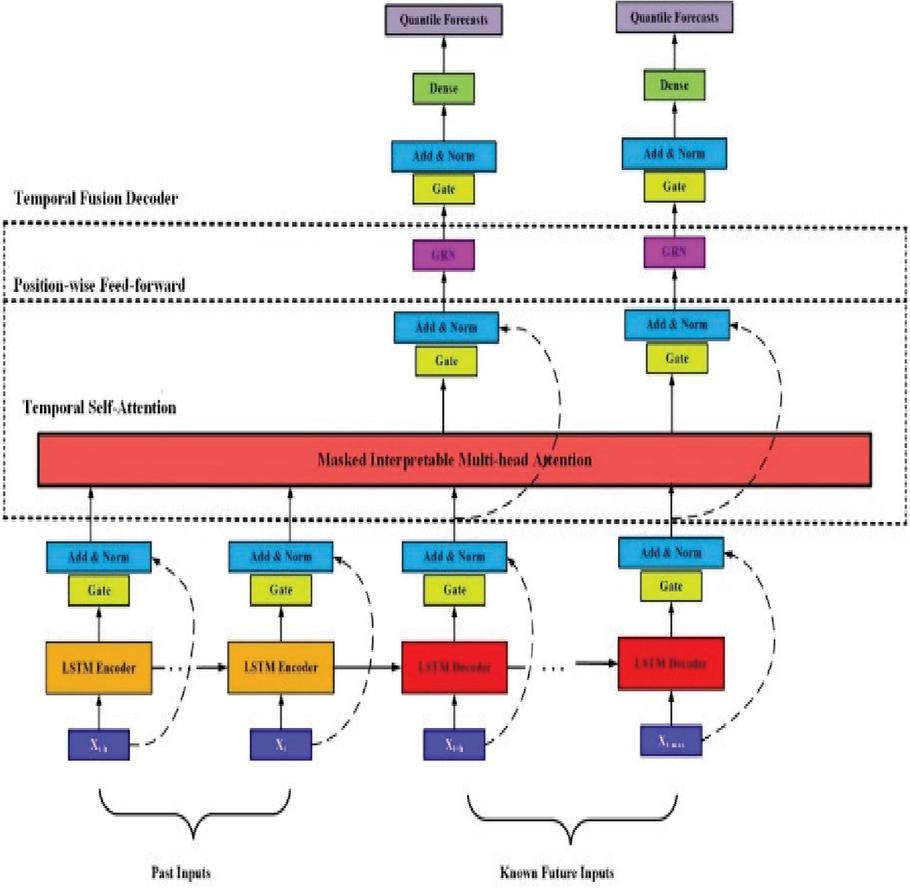
Figure 2 TFT-LSTM architecture.
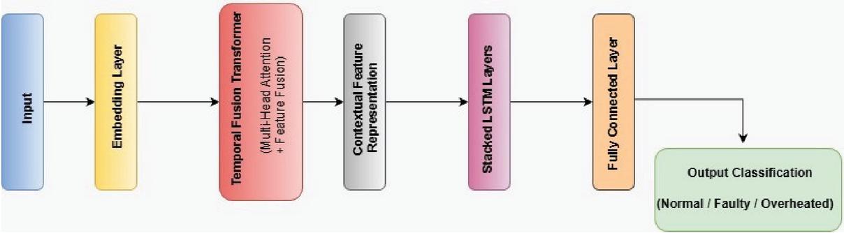
Figure 3 Hybrid TFT–LSTM model showing data flow.
Figure 3 illustrates the structured data flow within the proposed hybrid framework. Time-series inputs are first transformed through an embedding layer and processed by the Temporal Fusion Transformer for attention-based feature extraction and temporal fusion. The contextual embeddings generated by the TFT module are subsequently forwarded to stacked LSTM layers for sequential refinement and memory modeling. This two-stage processing enables both global temporal attention and progressive sequence learning. The final classification is performed through a fully connected output layer. The schematic clarifies the integration mechanism between attention-driven fusion and recurrent modeling components.
Pseudocode 1: TFT-LSTM # Step 1: Data Preprocessing Preprocess the dataset:
– Handle missing values
– Normalize data using Min-Max Scaling
– Encode categorical features using Label Encoding
– Split data into training and testing sets
# Step 2: Define the Hybrid Model (TFT-LSTM) Initialize the TFT model:
– Input historical data
– Use attention mechanisms and gated residual networks to capture long-range dependencies
Initialize the LSTM model:
– Use sequential data from TFT output
# Step 3: Combine TFT and LSTM Connect the output of TFT to the LSTM model:
– Feed processed data (TFT output) into the LSTM neural network
– Apply LSTM layers to detect faults in the grid
# Step 4: Train the Model Train the hybrid TFT-LSTM model:
– Use training data to optimize model parameters
– Use categorical cross-entropy as the loss function for classification
– Apply backpropagation and optimization techniques (SHO)
# Step 5: Evaluate the Model # Step 6: Predict Faults Use the trained model to predict faults:
– Input real-time data (voltage, current, frequency) into the model
– Classify the system state as “Normal,” “Faulty,” or “Overheated.”
# Step 7: Output Results Return the classification results:
– Print the predicted fault class and confidence score
– If a fault is detected, trigger a maintenance or corrective action
3.5 Employing SHO for Model Optimization
During the process of applying SHO as part of the optimization process, it will use the SHO optimize the hyperparameters of model to the point where we can get optimal fault detection and prediction, which is an important aspect of a smart power grid. In the SHO data optimization process, SHO uses iteration to generate a population of candidate solutions and then comparing their performance based on the objective function of error or accuracy as the criteria. The algorithm utilizes multi-faceted performance data while maintaining a dynamic balance of exploration and exploitation to the solution space. It allows the algorithm to search and conduct analysis on hyperparameter configurations of solutions for exploration purposes, as well as, some refinement of the best performing results. Over time, the SHO algorithm will converge on the optimal set of hyperparameters which minimizes the loss function of the model, meaning that SHO has adapted better to the dynamics of a technically complex power grid data for a fault detection model to be. The ultimate goal here is that by using SHO to optimize the model hyperparameters we can improve the performance of fault detection systems, and allow for predictive and pre-emptive action in relevant areas of power grid operations and disturbances.
The Spotted Hyena Optimizer was configured with a population size of 20 candidate solutions and executed for 50 optimization iterations. The selected population size ensures adequate diversity within the search space, enabling comprehensive exploration of hyperparameter combinations. The iteration count was determined to balance convergence stability and computational efficiency. This configuration reduces the likelihood of premature convergence and enhances the probability of escaping local optima. Such parameter settings support robust and reliable hyperparameter optimization within the proposed framework.
3.5.1 Input
The Input step is the step in which we initialize the population of candidate solutions, where every solution is a possible set of hyperparameters for the fault detection model (TFT and LSTM). After the solutions have been initialized, the population is evaluated based on fitness. To define fitness, it uses the ML model with the current hyperparameters (most often the loss function). It is given in Equation (19).
| (19) |
Where: represents the ith solution, N is the population size.
3.5.2 Objective function
The Measure of Fit determined by the objective function indicates how well a hyperparameter set (a solution) was doing in terms of model accuracy or error in relation to the problem in the loss function (categorical cross-entropy). The objective function is just a way to measure the fitness of all candidate solutions and guide the SHO problem to the best hyperparameter set, which will minimize the loss and optimize fault detection and prediction in the model. It is given in Equation (20).
| (20) |
Where: L is the loss function, is the predicted output, is the true output label.
3.5.3 Hunting behaviour of spotted hyenas
The Pursuing of Prey: When a hyena hunts prey (in this case, solutions) it will take into account where the prey is located and the velocity of the prey; it attempts to get closer to the optimal solution.
The Interacting Between Hyenas: The population of hyenas interacts with one another to exchange information and to move towards areas of the search space that may provide better solutions.
The Leadership and Ambush strategies: Hyenas pursue the best solutions in the population (leaders), while some pursue more aggressive ambush strategies. It is given in Equation (21).
| (21) |
Where: is the ith position, is the best position, r is a random factor.
3.5.4 Exploration and exploitation balance
With this step we ensure that the optimization process is both exploring and refining, exploring new areas of solution space and refining areas of the solution space that have produced best solutions so far. By dynamically adjusting the exploration coefficient , it ensures that it can anyhow optimise hyperparameters for models while still searching for each model’s optimal hyperparameters. A balance in exploration and exploitation avoids premature convergence while also guaranteeing a full search of the most effective configurations for fault detection models. It is given in Equation (22).
| (22) |
Where: is updated iteratively.
3.5.5 Convergence criteria
The algorithm considers the optimization process converged if there has been little improvement in the objective function, or if a predetermined number of iterations has been reached, and the algorithm takes the best solution for the fault detection model. It is given in Equation (23).
| (23) |
Where: is the ith fitness value, is the previous fitness value.
3.5.6 Final optimization result
The Final Optimization Result details the best solution selected from the entire set of evaluations in the iterative optimization process and represents the best hyperparameters for the fault detection model. The optimized hyperparameters were used to configure the TFT-LSTM model with optimized hyperparameters that would improve the accuracy of fault prediction and classification in the power grid system.
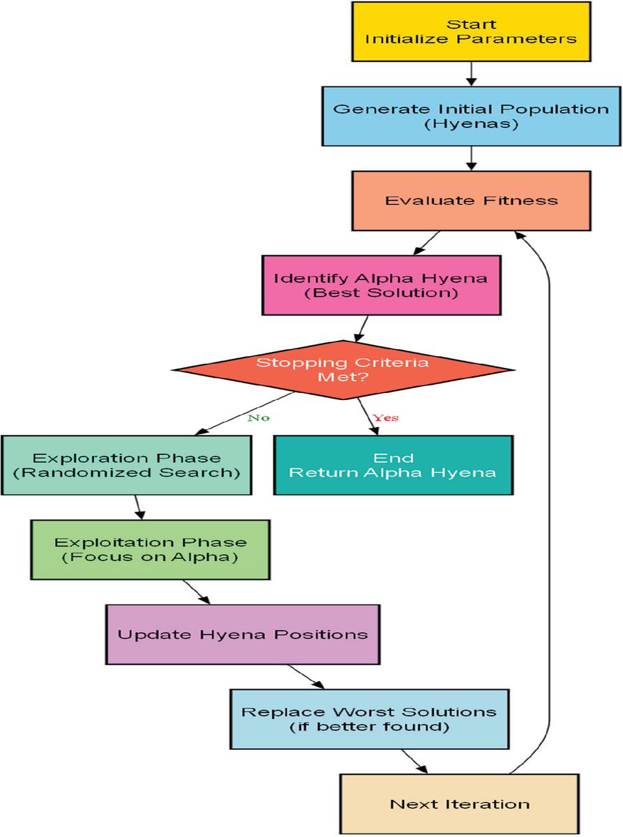
Figure 4 Flow diagram of SHO.
The flowchart in Figure 4 illustrates the structural operation of the SHO algorithm inspired by hyena social hunting behaviour. The algorithm starts with the setting of algorithm parameters and the generation of a population of candidates to be explored, here referred to as hyenas. The fitness of the hyenas is determined and the best one is identified as the alpha hyena. The algorithm evaluates whether there is a stopping condition; if there is no stopping condition, the algorithm proceeds through the exploration stage – allowing for an increased chance for randomness so as to allow diversity – and then through exploitation – the hunt comes near the alpha hyena’s location in search of better hyenas. The algorithm calculates new positions for the hyenas, replaces worse solutions if better solutions are found, and the process loops over and over until convergence occurs or a stopping condition is met. In which case the best solution discovered (the alpha as previously identified) is returned. The design illustrates a balance between diversification and intensification such that SHO is able to navigate very complex search environments efficiently.
Pseudocode 2: SHO # Step 1: Initialize the SHO Algorithm Initialize the population of candidate solutions (hyperparameters):
– Define hyperparameters to optimize
– Randomly generate initial solutions for the hyperparameters
– Set the maximum number of iterations for optimization
# Step 2: Define the Fitness Function Define the fitness function to evaluate the candidate solutions:
– For each candidate solution, build the model with the proposed hyperparameters
– Train the model on the training dataset
– Calculate the fitness score of the model
– The fitness score determines how well the candidate solution performs
# Step 3: Evaluate Candidate Solutions For each candidate solution in the population:
– Evaluate its performance using the fitness function
– Assign a fitness score to each solution based on the model’s performance
# Step 4: Update the Positions (Optimization Process) For each iteration:
– Determine the best solution in the current population (leader hyena)
– Update the positions of other hyenas based on the leader’s position:
– Pursue prey: Move toward better solutions (leaders)
– Exploration: Randomly search other areas of the solution space
– Exploitation: Focus on refining the best solutions found so far
– Update the velocities and positions of candidate solutions based on:
– The position of the best candidate solution (leader)
– A random exploration factor
# Step 5: Apply Update Rules For each candidate solution:
– Apply the hunting and ambush strategies:
– Hyenas move toward the best solution (exploitation)
– Random movements are allowed (exploration)
– Update the fitness values and positions of each solution
# Step 6: Check Convergence Criteria If the fitness score of the best solution converges (minimal improvement over iterations):
– Stop the optimization process
– Select the best hyperparameters (solution) as the optimal configuration
# Step 7: Final Optimization Result Output the optimized hyperparameters:
– Use the best solution found to configure the model (TFT-LSTM)
# End of optimization process
4 Results and Discussion
This section describes how the model was assessed with regards to its metrics and graphical analyses. It highlights the most relevant inputs and their importance, distributions, features, interrelations, and overall, how well and dependably the model predicts outcomes. With the various performance metrics, this part assesses the operational states classification and fault detection capabilities of the model in the system.
4.1 Evaluation of Prediction and Classification
The histograms of the four electrical and environmental variables of interest Voltage, Current and Power Load, and Temperature are provided in Figure 5. The histograms suggest a lot of information related to the operational conditions and environmental conditions of the monitored system. The histograms of voltage and current have relatively uniform distributions with some visible multimodality suggesting that there are fluctuations around multiple operating levels, while the Power Load distribution appears to be much more homogeneous, which is consistent with the notion that the system is requiring energy to do work within a narrow range of 50–53 MWM. In the case of Temperature, there is the potential that distributions are bimodal, which may be due to time-of-day temperature changes or shifts in the operating conditions of the equipment. Further details with respect to these distributions can be observed through the inserted KDE curves, which can facilitate further statistical analysis, and assist in identifying suitable conditions for optimizing the system beyond normal operating parameters, should that be necessary.
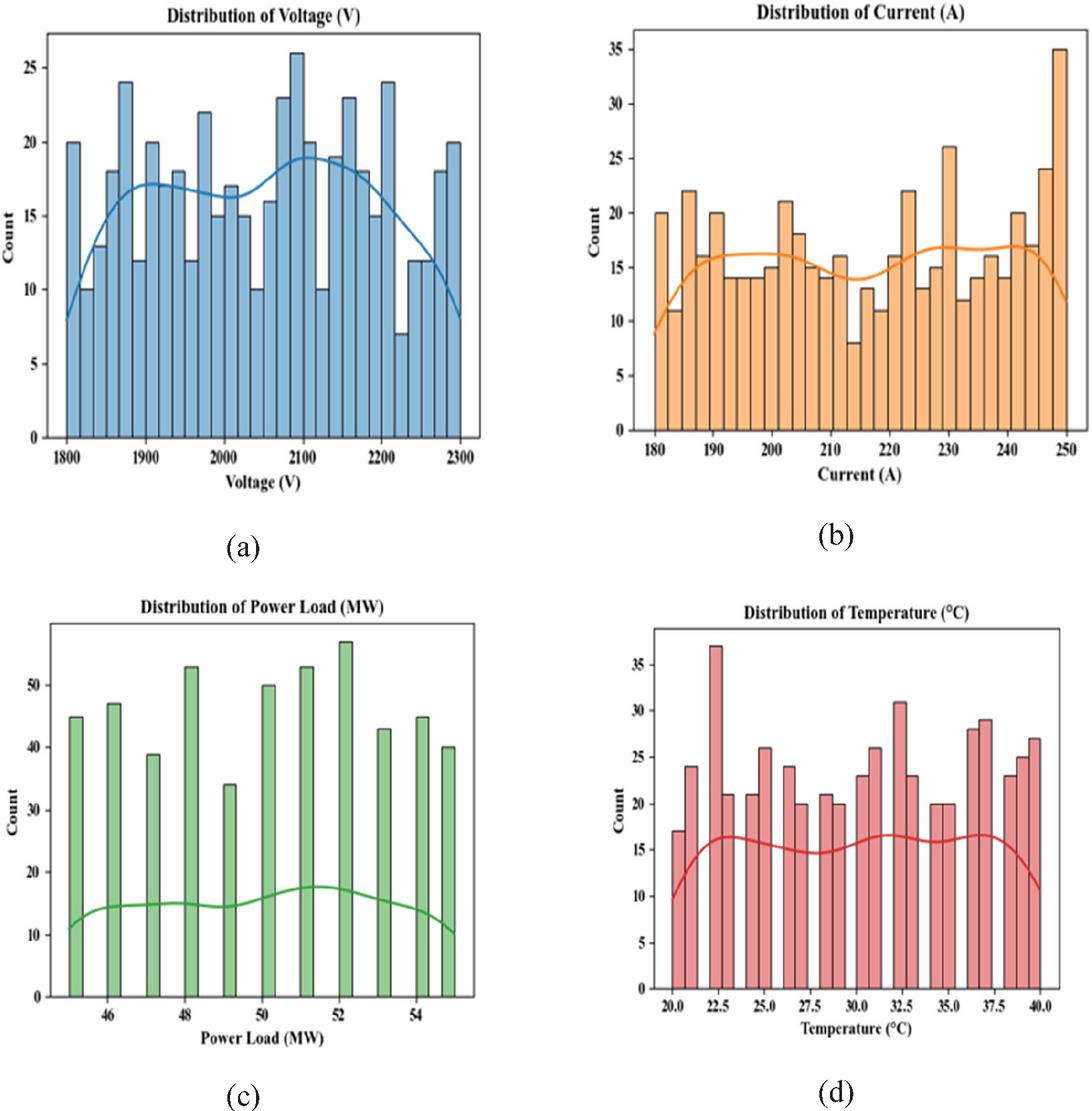
Figure 5 Distribution of (a) voltage (b) current (c) power Load (d) temperature.
The importance scores for each feature resulting from a predictive model targeting factors influencing system performance or failure is depicted in Figure 6. It is clear that Voltage is the most important feature used in the model, followed closely by Current and Power Load, suggesting that the electrical characteristics used in the model are the most dominant parameters predicted with this model. Environmental and operational factors, such as Temperature and Wind Speed, are of moderate importance since they were direct effects of system dynamics that were indirectly observed. Component Health was also significant, which is important to highlight since monitoring physical condition is still a critical factor. Downtime or fault duration was least important when ranked in terms of prediction.
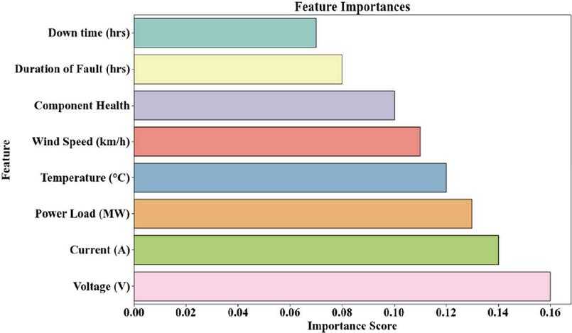
Figure 6 Feature importance.
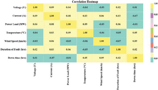
Figure 7 Correlation heatmap.
The correlation heatmap showing correlations among several operational and environmental characteristics is given in Figure 7. The matrix demonstrates that most characteristics have weak correlations to each other with low absolute values of the correlation coefficients. More specifically, voltage, current, and power load all have virtually no correlation to each other indicating relative independence in terms of the system context. Likewise, the environmental characteristics including temperature and wind speed all have limited correlation with operational characteristics indicating that they function in separate influence domains. Of the correlations indicated, the strongest correlations are modest and mostly self-referential (i.e., the diagonal values of 1.00) and all off-diagonal values are near zero. Given this overall weak correlation structure, it is important to realize that there are limited linear dependencies between the characteristics, and this shows that multivariate analysis approaches will be necessary in modelling or diagnostic applications. The weak linear correlations observed among input features indicate limited direct inter-variable dependency within the dataset. Such low correlation patterns reduce the effectiveness of shallow classifiers that rely primarily on explicit linear relationships. Fault behavior in power systems often evolves through nonlinear and time-dependent interactions that cannot be captured through static feature mapping alone. Deep temporal architectures are capable of modeling higher-order dependencies across sequential observations, thereby extracting latent dynamic patterns. The combined TFT–LSTM framework enables both attention-based feature fusion and sequential memory learning under weak interdependency conditions. This characteristic justifies the adoption of deep historical modeling for robust fault classification.
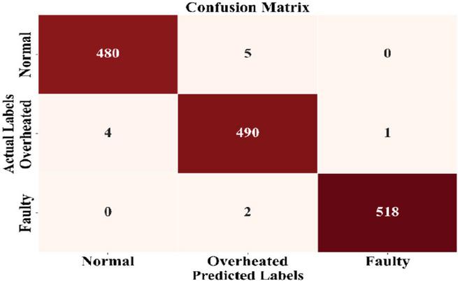
Figure 8 Confusion matrix.
The confusion matrix in assessing the performance of our multi-class classification model that is created to classify system states as Normal, Overheated, or Faulty and it is depicted in Figure 8. The model has high prediction accuracy over the three classes, with most samples correctly classified: 480 normal, 490 overheated, and 518 faulty. The misclassified samples were few. Only five normal were classified as overheated and those two faulty were classified as overheated. There were no normal misclassified as faulty and vice versa, which stands to reason as it expected to not classify the normal operational state with the faulty state since they are distinctly different. The relatively low number of false positive and false negative values suggests a high level of precision and recall, making this model suitable for reliance within fault detection in real-time and maintenance scheduling in critical systems.
4.2 Evaluation of Performance of Model
The graph displayed in Figure 9 shows a plot of model accuracy dependent upon the training epochs. The trend of accuracy was uniformly increasing, eventually converging towards a high number of accuracies. The model “learned” the data quickly, refined, and improved, with the early epochs showing a slight amelioration in accuracy, but then sinking more slowly into a plateau of high accuracies.
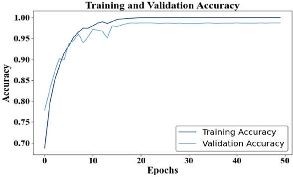
Figure 9 Model accuracy.
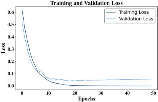
Figure 10 Model loss.
The mapping of model loss across the training epochs is given in Figure 10. The loss curves, all trend downward, indicating that model performance increased with training epochs. The overall shape of the curves is notable, with the loss dropping rapidly during the early epochs, and then levelling out over the next few epochs, demonstrating a good learning process and convergence. The final loss values were low overall suggesting a good overall fit (low error) and the model fitting the errors in the training data.
The precision-recall curve was illustrated in Figure 11, and it shows the capacity of system to achieve a balance between precision and recall for different classification thresholds.
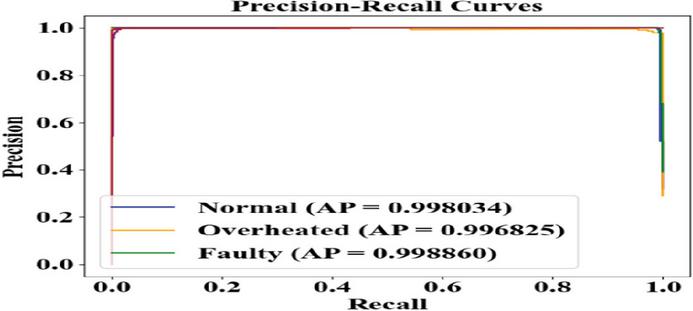
Figure 11 Precision-recall curve.
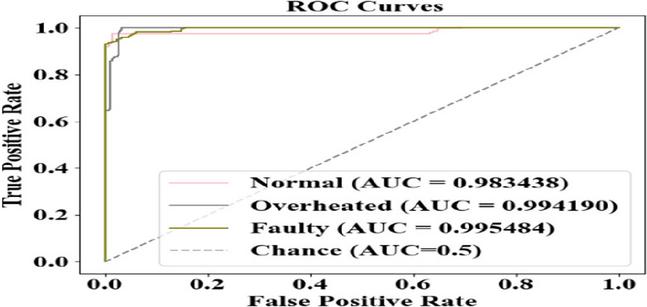
Figure 12 ROC curve.
The ROC curve illustrating the classification performance of the model with respect to the threshold is depicted in Figure 12. The curve is relatively close to the top-left corner, indicating a high TPR, and a low FPR. It can generalize that there is excellent ROC performance based on this strong ROC performance, and the model can sufficiently discriminate between the various states of the system. During ROC and precision–recall evaluation, classification probability thresholds were systematically varied between 0 and 1 to analyze performance sensitivity across decision boundaries. The optimal threshold was determined using the maximum Youden’s Index criterion, which maximizes the difference between true positive rate and false positive rate. This approach ensures a balanced trade-off between sensitivity and specificity under operational conditions. In addition, precision–recall behavior was examined to account for potential class imbalance effects. Explicit threshold selection strengthens evaluation transparency and provides a realistic basis for deployment-oriented decision making.
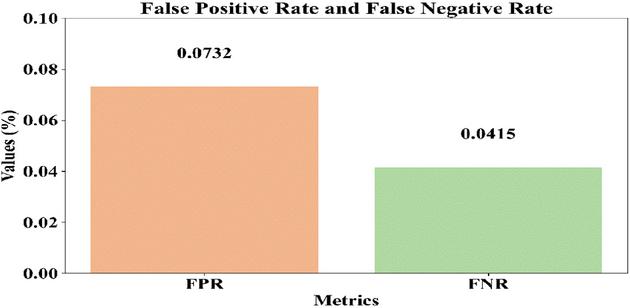
Figure 13 FPR and FNR.
Comparative bar chart of the FPR and FNR, displaying the classification errors made by the model, is depicted in Figure 13. The FPR is at 0.0732% and the FNR is at 0.0415%. The FPR is slightly more than the FNR, showing the model is slightly more likely to classify a non-faulty instance as faulty than it is to miss an actual fault. Overall, both the FPR and FNR are both low, indicating the model is highly robust and it makes an insignificant amount of misclassification, which is critical for successful monitoring and time-based decision making to avoid costly failures in sensitive operations.
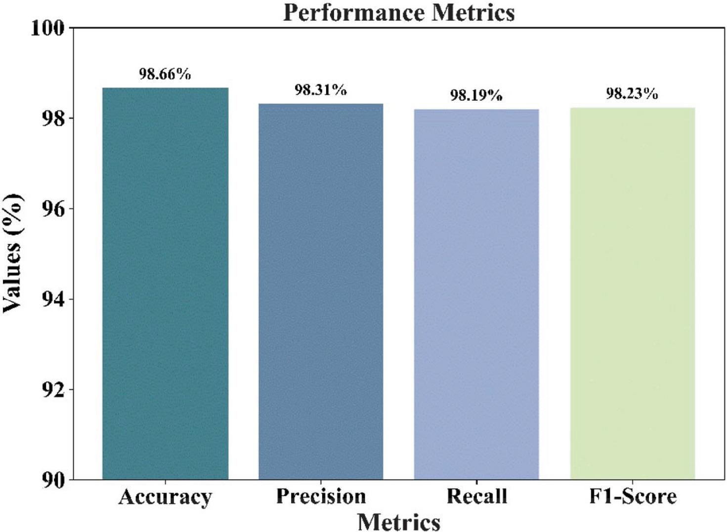
Figure 14 Performance metrics.
The summary of the results for the model using principal evaluation metrics is depicted in Figure 14. Of the four metrics, Accuracy was the highest at 98.66%, verifying that the model classified instances correctly overall. Precision (98.31%) and Recall (98.19%) clustered closely to the model had reasonable balance in performance and was minimizing false positives and false negatives appropriately, which is paramount for validating fault detection and diagnosis on critical systems. The same is true for F1-Score (98.23%).
4.3 Comparison with Existing Methods
The comparison between the current model, TFT-LSTM, with various other forms of fault detection including DT, GNB and SE-CDAE is given in Table 1. The current model provided superior performance when compared to all other methods with an accuracy of 98.66%, which is greater than the next best, the SE-CDAE classification method with an accuracy of 97.98%. In addition, the TFT-LSTM model provided better performance with respect to the performance metrics. This demonstrates that the model is a robust and effective approach for fault detection. The GNB model was significantly worse than all metrics in this paper, indicating the limitations of this model to generate the complexity of the data when observing power grid faults, overall, the accuracy indicates the TFT-LSTM model was a more robust and accurate method to detect and predict power systems fault.
Table 1 Comparison with existing methods
| Methods | Accuracy (%) | Precision (%) | Recall (%) | F1-Score (%) |
| DT [33] | 97.42 | 97.43 | 97.42 | 97.42 |
| GNB [33] | 83.49 | 83.23 | 83.49 | 83.31 |
| SE-CDAE [34] | 97.98 | 94.83 | 96.28 | 97.35 |
| Proposed TFT-LSTM | 98.66 | 98.31 | 98.19 | 98.23 |
5 Discussion
The results show that the proposed method, the TFT-LSTM model, is significantly better than current fault detection methods in power systems, which include DT, GNB, and SE-CDAE. The TFT-LSTM model is the only one with an accuracy of 98.66% and consistently outperforms other methods. Thus, the hybrid model’s combination of TFT-LSTM neural networks was able to achieve the most accurate classification of faults by minimizing false positive and negative classifications while also being used for prediction. The hybrid model with the use of TFT-LSTM taken together was able to capture long-term temporal dependencies and sequential patterns exhibited in time series data, which results in better fault detection and identification. It is worth noting that the great improvement over traditional methods show that separating and merging the key concepts to advanced techniques of attention mechanisms and gated residual networks still provides value as separate techniques to work on modern ML systems.
In contrast, models, such as GNB and SE-CDAE, performed worse with recall and F1-score, demonstrating that they seem to be incapable of handling the inherent complexity and variability of power grid data. Even though SE-CDAE performed well, our proposed TFT-LSTM model with higher precision and recall seems to be better at detecting faults and making accurate predictions, which are essential for preventing failure and reducing downtime. In summary, the results provide an understanding of the validated capability and effectiveness of the TFT-LSTM model to support fault detection platforms in power networks and additionally demonstrate the opportunity for a smarter alternative for predictive maintenance and stability of modern energy systems.
6 Conclusion and Future Works
In conclusion, a novel fault detection and classification technique is proposed for power grids, employing hybrid TFT-LSTM neural networks. The present approach to fault detection is vulnerable to the highly dynamic nature and complexity of the modern phenomena being studied, especially in the presence of renewable energy sources. The TFT-LSTM model evidences very strong improvement in the fault detection accuracy as compared to classical machine learning techniques. The results show that the hybrid model produces an accuracy of 98.66%, which is higher than that obtained by decision trees and support vector machines. Also, the high-performance metrics values prove the greatness of this method, putting it forward as an effective technique for online fault detection and maintenance actions on power grids.
Although the proposed model demonstrates promising capability, there is still a lot of opportunity to advance the development. One avenue for future work could be the integration of additional features, such as weather data and real-time operational conditions that may further enhance the model’s capability to adapt to different grid environments. DRL could instead be exploited to fine-tune the model performance in dynamic grid conditions. Moreover, there is the need to work on its scalability to large-scale power systems with more diverse fault types and environmental factors. Also, it would be nice to have a lightweight version of the model that can run on edge devices to serve real-time applications with constrained computational resources. Giving explainable AI treatment to the decision-making process of the TFT-LSTM model would further aid in engendering transparency and trust, which are central to its technology adoption in critical infrastructure.
Declarations
Funding
The authors did not receive support from any organization for the submitted work.
Conflict of Interest
The authors declare that they have no conflict of interest.
Ethics Approval
Not applicable.
Consent to Participate
Not applicable.
Consent to Publish
Not applicable.
Data Availability
Data sharing does not apply to this article as no new datasets were generated or analyzed during the current study.
Code Availability
Not applicable.
Authors’ Contributions
• Qinghua Chen: Conceptualization, Methodology, Writing – original draft, Supervision.
• Tao Xu: Data curation, Validation, Writing – review & editing.
• Cheng Zhou: Investigation, Formal analysis, Software implementation.
• Yating Wang: Visualization, Resources, Writing – review & editing.
Acknowledgment
The authors would like to thank the Economic and Technical Research Institute of State Grid Jiangxi Electric Power Co., Ltd., Nanchang, China, for providing the resources and technical support that made this research possible.
References
[1] Pourfaraj, M., et al.: A fault detection algorithm based on artificial neural network threshold selection in multi-terminal DC grids. IEEE Trans. Power Delivery 38(4), 2510–2520 (2023). https://doi.org/10.1109/TPWRD.2023.3244853.
[2] Roy, S., Debnath, S.: A wavelet-based PSD approach for fault detection and classification in grid-connected inverter-interfaced microgrid. Measurement 226, 114079 (2024). https://doi.org/10.1016/j.measurement.2023.114079.
[3] Zhou, M., Wang, J., Li, B.: ARG-Mask RCNN: An infrared insulator fault-detection network based on improved Mask RCNN. Sensors 22(13), 4720 (2022). https://doi.org/10.3390/s22134720.
[4] Zhou, Y., Lin, Z., Tu, L., Song, Y., Wu, Z.: Big data and knowledge graph-based fault diagnosis for electric power systems. EAI Endorsed Trans. Ind. Net. Intel. Syst. 9(32), e1 (2022). https://doi.org/10.4108/eetinis.v9i32.1268.
[5] Jasim, M., Jasim, B.H., Neagu, B.C., Alhasnawi, B.N.: Coordination control of a hybrid AC/DC smart microgrid with online fault detection, diagnostics, and localization using artificial neural networks. Electronics 12(1), 187 (2022). https://doi.org/10.3390/electronics12010187.
[6] Montoya, R., Poudel, B.P., Bidram, A., Reno, M.J.: DC microgrid fault detection using multiresolution analysis of traveling waves. Int. J. Electr. Power Energy Syst. 135, 107590 (2022). https://doi.org/10.1016/j.ijepes.2021.107590.
[7] Roy, S., et al.: Deep learning-based relay for online fault detection, classification, and fault location in a grid-connected microgrid. IEEE Access 11, 62674–62696 (2023). https://doi.org/10.1109/ACCESS.2023.3285768.
[8] Yahyaoui, Z., Hajji, M., Mansouri, M., Abodayeh, K., Bouzrara, K., Nounou, H.: Effective fault detection and diagnosis for power converters in wind turbine systems using KPCA-based BiLSTM. Energies 15(17), 6127 (2022). https://doi.org/10.3390/en15176127.
[9] Bramareswara Rao, S.N.V., Kumar, Y.V.P., Amir, M., Muyeen, S.M.: Fault detection and classification in hybrid energy-based multi-area grid-connected microgrid clusters using discrete wavelet transform with deep neural networks. Electr. Eng. (2024). https://doi.org/10.1007/s00202-024-02329-4.
[10] Alhanaf, S., Balik, H.H., Farsadi, M.: Intelligent fault detection and classification schemes for smart grids based on deep neural networks. Energies 16(22), 7680 (2023). https://doi.org/10.3390/en16227680.
[11] Sebastian, P.K., D.K.: Internet of Things based smart energy meter with fault detection feature and theft detection. In: Proc. Int. Conf. Electronics and Renewable Systems (ICEARS), pp. 494–500. IEEE, Tuticorin (2022). https://doi.org/10.1109/ICEARS53579.2022.9751828.
[12] Cichoń, A., Włodarz, M.: OLTC fault detection based on acoustic emission and supported by machine learning. Energies 17(1), 220 (2023). https://doi.org/10.3390/en17010220.
[13] Nguyen, L.H., Vu, T.V., Nguyen, T.-T., Panwar, M., Hovsapian, R.: Spatial-temporal recurrent graph neural networks for fault diagnostics in power distribution systems. IEEE Access 11, 46039–46050 (2023). https://doi.org/10.1109/ACCESS.2023.3273292.
[14] Zahraoui, Y., Alhamrouni, I., Hayes, B.P., Mekhilef, S., Korõtko, T.: System-level condition monitoring approach for fault detection in photovoltaic systems. In: Haque, A., Mekhilef, S. (eds.) Fault Analysis and its Impact on Grid-Connected Photovoltaic Systems Performance, pp. 215–254. Wiley, Hoboken (2022). https://doi.org/10.1002/9781119873785.ch7.
[15] Mahmoud, R.A.: Transmission line faults detection and classification using new tripping characteristics based on statistical coherence for current measurements. Sci. Rep. 15(1), 8487 (2025). https://doi.org/10.1038/s41598-025-87577-5.
[16] Almasoudi, F.M.: Enhancing power grid resilience through real-time fault detection and remediation using advanced hybrid machine learning models. Sustainability 15(10), 8348 (2023). https://doi.org/10.3390/su15108348.
[17] Najafzadeh, M., Pouladi, J., Daghigh, A., Beiza, J., Abedinzade, T.: Fault detection, classification and localization along the power grid line using optimized machine learning algorithms. Int. J. Comput. Intell. Syst. 17(1), 49 (2024). https://doi.org/10.1007/s44196-024-00434-7.
[18] Hosamo, H.H., Svennevig, P.R., Svidt, K., Han, D., Nielsen, H.K.: A digital twin predictive maintenance framework of air handling units based on automatic fault detection and diagnostics. Energy Build. 261, 111988 (2022). https://doi.org/10.1016/j.enbuild.2022.111988.
[19] Shakiba, F.M., Shojaee, M., Azizi, S.M., Zhou, M.: Real-time sensing and fault diagnosis for transmission lines. Int. J. Netw. Distrib. Intell., 36–47 (2022). https://doi.org/10.53941/ijndi0101004.
[20] Zhang, K.: Online fault diagnosis for single-phase PWM rectifier using data-driven method. CPSS Trans. Power Electron. Appl. 7(1), 49–57 (2022). https://doi.org/10.24295/CPSSTPEA.2022.00005.
[21] Sridharan, N.V., Sugumaran, V.: Convolutional neural network based automatic detection of visible faults in a photovoltaic module. Energy Sources, Part A: Recovery, Utilization, and Environmental Effects 47(1), 6270–6284 (2025). https://doi.org/10.1080/15567036.2021.1905753.
[22] Ding, Y., Chen, Z., Zhang, H., Wang, X., Guo, Y.: A short-term wind power prediction model based on CEEMD and WOA-KELM. Renew. Energy 189, 188–198 (2022). https://doi.org/10.1016/j.renene.2022.02.108.
[23] Mostafa, N., Ramadan, H.S.M., Elfarouk, O.: Renewable energy management in smart grids by using big data analytics and machine learning. Mach. Learn. Appl. 9, 100363 (2022). https://doi.org/10.1016/j.mlwa.2022.100363.
[24] Chen, X., Wang, M., Zhang, H.: Machine learning-based fault prediction and diagnosis of brushless motors. Eng. Appl. 4(3), 130–142 (2024). https://doi.org/10.26855/ea.2024.07.004.
[25] Zeng, N., Wu, P., Wang, Z., Li, H., Liu, W., Liu, X.: A small-sized object detection oriented multi-scale feature fusion approach with application to defect detection. IEEE Trans. Instrum. Meas. 71, 1–14 (2022). https://doi.org/10.1109/TIM.2022.3153997.
[26] Khan, Z.A., Hussain, T., Haq, I.U., Ullah, F.U.M., Baik, S.W.: Towards efficient and effective renewable energy prediction via deep learning. Energy Rep. 8, 10230–10243 (2022). https://doi.org/10.1016/j.egyr.2022.08.009.
[27] Swana, E.F., Doorsamy, W., Bokoro, P.: Tomek Link and SMOTE approaches for machine fault classification with an imbalanced dataset. Sensors 22(9), 3246 (2022). https://doi.org/10.3390/s22093246.
[28] Albarakati, J., et al.: multi-agent-based fault location and cyber-attack detection in distribution system. Energies 16(1), 224 (2022). https://doi.org/10.3390/en16010224.
[29] Baker, M., Fard, A.Y., Althuwaini, H., Shadmand, M.B.: Real-time AI-based anomaly detection and classification in power electronics dominated grids. IEEE J. Emerg. Sel. Top. Ind. Electron. 4(2), 549–559 (2023). https://doi.org/10.1109/JESTIE.2022.3227005.
[30] Huang, L., Wu, C., Zhou, D., Blaabjerg, F.: A power-angle-based adaptive overcurrent protection scheme for grid-forming inverter under large grid disturbances. IEEE Trans. Ind. Electron. 70(6), 5927–5936 (2023). https://doi.org/10.1109/TIE.2022.3199906.
[31] Conte, F., D’Agostino, F., Gabriele, B., Schiapparelli, G.-P., Silvestro, F.: Fault detection and localization in active distribution networks using optimally placed phasor measurements units. IEEE Trans. Power Syst. 38(1), 714–727 (2023). https://doi.org/10.1109/TPWRS.2022.3165685.
[32] Power system faults dataset. Kaggle. Accessed 8 May 2025. Available: https://www.kaggle.com/datasets/ziya07/power-system-faults-dataset.
[33] Venkata, P., Pandya, V., Vala, K., Sant, A.V.: Support vector machine for fast fault detection and classification in modern power systems using quarter cycle data. Energy Rep. 8, 92–98 (2022). https://doi.org/10.1016/j.egyr.2022.10.279.
[34] Veeramachaneni, V., Husain, S.O., Khanna, V., Pareek, P.K., Bhuvaneshwari, P.: Fault detection and classification in power grids using Shannon entropy with convolution distributed autoencoder. In: Proc. Int. Conf. Mobile Networks and Wireless Communications (ICMNWC), pp. 1–5. IEEE, Tumkuru (2024). https://doi.org/10.1109/ICMNWC63764.2024.10872059.
Biographies

Qinghua Chen holds a Master’s degree and is currently a Senior Engineer. His primary research focuses on power systems and automation, with extensive experience in technical R&D and management within the field.

Tao Xu is a Senior Engineer holding a Master’s degree. He specializes in transmission line technology and possesses deep theoretical knowledge and practical expertise in power transmission engineering.

Cheng Zhou is a Senior Engineer with a Master’s degree. His research interests lie in Information and Communication Engineering, focusing on the integration and innovation of communication technologies in the power sector.

Yating Wang is a Senior Engineer holding a Master’s degree. She specializes in power systems and automation, with a strong research background in power system operation and control mechanisms.
Distributed Generation & Alternative Energy Journal, Vol. 41_4, 857–898
doi: 10.13052/dgaej2156-3306.4142
© 2026 River Publishers