Industrial Electricity Load Forecasting Considering Periodic Features and Inter-Industry Associations
Bo Zhao, Ying Zheng*, Ying Hao, Xin Li and Jiaheng Yang
School of Automation, Beijing Information Science and Technology University, Beijing 100192, China
E-mail:994198992@qq.com
*Corresponding Author
Received 22 September 2025; Accepted 15 April 2026
Abstract
Industrial electricity load forecasting is crucial for the stable operation of power systems and energy management. However, the complex temporal patterns and dynamic interdependencies between loads from different industries make it challenging for traditional forecasting methods to model effectively. To address this, this paper proposes a forecasting model based on an inter-industry association dynamic graph neural network that integrates periodic features. The proposed method uses the Time2Vector block to adaptively capture multiple periodic fluctuations in the load sequence, and combines this with the cointegration relationship and error correction mechanism from the Vector Error Correction Model (VECM) to quantify the association strength between industries. Each industry is represented as a node, and the association strengths define the edges and their weights. Thus, this forms a Dynamic Inter-industry Association Graph (DIAG). This graph is then integrated into a Dynamic Spatial-Temporal Aware Graph Neural Network framework. As a result, the Inter-industry Association Dynamic Graph Neural Network (IADGNN) is formed. This model captures the complex dynamic characteristics of electricity loads across different industries. Test cases based on industrial load data from one province in China show that this method significantly outperforms traditional models in terms of forecasting accuracy, providing a novel solution for addressing the complex industrial load forecasting problem.
Keywords: Industrial electricity load forecasting, time2vector, periodic features, VECM, inter-industry association dynamic graph neural network.
1 Introduction
The “dual-carbon” policy has accelerated electrification and the development of renewable energy, increasing overall electricity demand and introducing more concentrated and variable load patterns, thereby intensifying fluctuations in the power system [1, 2]. The 14th Five-Year Plan for China’s Modern Energy System explicitly proposes enhancing the elasticity of power loads, promoting interaction on the demand side [3, 4]. This has resulted in stronger time-variant and coupled characteristics in the load profiles across different sectors. Accurate prediction of electricity demand in various industries is crucial not only for improving the efficiency and stability of power system operations [5], but also for optimizing energy management, thereby advancing the goal of green and low-carbon development [6].
In recent years, with the rapid advancement of time series forecasting technologies, machine learning and deep learning-based approaches have become prominent in the field of power load forecasting [7]. Existing studies primarily focus on two dimensions: one is the total load forecasting for a specific region or system, and the other targets industry-specific or user-specific load modeling.
In the area of regional load forecasting, [8] compared the performance of hybrid Convolutional Neural Network and Recurrent Neural Network (CNN-RNN), CNN and Long Short-Term Memory (CNN-LSTM), and CNN and Gated Recurrent Unit (CNN-GRU) models using data from eight U.S. states. In [9], an attention-enhanced Seq2Seq-LSTM model was proposed for Brazil’s national load, effectively capturing long-term dependencies. Reference [10] proposes an improved pelican optimization algorithm (IPOA) to optimize the extreme learning machine (ELM) for short-term power load forecasting in the Australian region. In [11], a Monte Carlo Neural Network (MCNN) was innovatively introduced to address uncertainty in power load forecasting for Queensland through probabilistic modeling. However, these studies generally treat the total regional load as a unified whole, failing to capture the distinct consumption behaviors of different industries. Meanwhile, the representation of temporal information still mainly relies on traditional time feature construction methods, which makes it difficult to adequately characterize the complex periodic and nonlinear variations in load time series. In recent years, the effective representation of time information has gradually become a key factor in improving forecasting accuracy. Time2Vector, as a time embedding method, has been widely applied to forecasting, anomaly detection, and time series analysis tasks in domains such as stock prediction, healthcare, and sales forecasting [12]. Compared with traditional time feature construction approaches, Time2Vector representations can significantly enhance the final predictive performance of models. By directly learning appropriate time functions from data, this method avoids the limitations of manually designed time features and can be seamlessly integrated into existing deep learning architectures at a relatively low implementation cost.
To address the heterogeneity of industrial load characteristics, researchers have developed a variety of industry-specific forecasting models. Given the high volatility and energy intensity of industrial loads, they are often the focus of modeling efforts. For instance, [13–16] proposed various approaches including an Empirical Mode Decomposition-Variational Mode Decomposition-Particle Swarm Optimization-Least Squares Support Vector Machine (EMD-VMD-PSO-LSSVM) decomposition model, a Particle Swarm Optimization optimized Back Propagation neural network, an ensemble learning-enhanced LSTM model, and a Temporal Convolutional Network and Light Gradient Boosting Machine (TCN-LightGBM) fusion model. These methods leverage signal decomposition, parameter adaptation, and feature extraction to improve forecasting accuracy. In the residential sector, [17] utilized Bayesian networks to model correlations among multi-household loads, while [18] proposed a model combining persistence-based autoregression (PAR), seasonal persistence regression (SPR), and neural networks (SPNN), along with an adaptive ensemble switching strategy. For transportation loads, [19] adopted artificial neural networks (ANN) to predict base and extreme peak loads, and [20] developed an attention-based deep learning model to forecast the charging load of electric vehicles. However, these studies are typically confined to single-industry scenarios, lacking exploration of inter-industry load correlations.
Some recent studies have attempted to explore multi-type load relationships from different perspectives. For example, [21] independently constructed forecasting models for different industries to capture load heterogeneity, which improved individual industry accuracy but overlooked potential cross-sector correlations. In [22], a bidirectional long short-term memory (BiLSTM)-based multi-task learning framework was proposed to jointly predict cold, heat, and electricity loads within the same energy system by sharing hidden features. However, the static parameter-sharing mechanism limits its ability to capture dynamic inter-industry coupling. Meanwhile, graph neural networks (GNNs) have emerged as powerful tools for spatiotemporal prediction, offering new insights for multi-source load modeling. Yet, their application remains limited to two main scenarios:
(1) Modeling geographical correlations across regions, such as in the MDST-GNN model proposed in [23], which built a spatial graph based on geographic proximity and integrated temporal and graph convolutions; [24] further introduces a spatiotemporal attention mechanism to capture the dynamic spatial correlations of load among geographically adjacent regions.
(2) Modeling user-level associations within a single industry, as in [25], where Pearson correlation and transfer entropy were used to build synchronous and causal graphs among residential users, through which the linear and nonlinear relationships in user load were mined based on the graph structures.
These methods, however, show clear limitations: It is evident that existing graph-based methods have significant limitations. In the context of industrial load forecasting, they can neither directly use geographical distance to construct static spatial graphs nor effectively capture the dynamic association between industries. Therefore, constructing a dynamic association graph structure suitable for inter-industry load becomes key to breaking through the bottleneck in forecasting accuracy.
To address the above issues, this paper proposes a multi-industry load forecasting model based on an inter-industry assiciation dynamic graph neural network integrated with periodic characteristics. The remainder of this paper is organized as follows: firstly, the temporal regularity characteristics and inter-industry association characteristics are thoroughly analyzed to lay a foundation for subsequent modeling; secondly, the model architecture and advantages are systematically elaborated, while the limitations of this framework in temporal feature representation and assiciation graph construction are analyzed; on this basis, the Time2Vector block is introduced, which relies on its advantage of adaptive learning of dynamic periodicities to solve the problem of single temporal feature representation and realize high-dimensional temporal feature embedding of multi-industry loads; the Vector Error Correction Model (VECM) is adopted to analyze the long-term periodic correlations and short-term fluctuation characteristics of industrial loads, so as to construct a graph structure that captures inter-industry association characteristics; then, the above blocks are integrated to build an inter-industry assiciation dynamic graph neural network model integrated with periodic characteristics, achieving synergistic modeling of temporal features and correlation characteristics; finally, based on the measured multi-industrial load data of a province in China, comparative and ablation Empirical studies are designed to demonstrate the superiority of the proposed model in prediction accuracy.
2 Related Work
2.1 Analysis of Industrial Power Load Characteristics
2.1.1 Temporal pattern characteristics
There exists a significant correlation between the future power load of a specific industry during a given time period and its historical load levels. This temporal evolution of load patterns is referred to as the temporal pattern characteristics of industrial power load. To validate this property, typical load curves of various industries were plotted based on industrial load data of a province in China, and the load variation patterns across different time periods were compared.

Figure 1 Weekly load curves for four industries.
For example, in service sectors such as Transportation, Warehousing and Postal; Information Technology Services; Wholesale and Retail; and Leasing and Business Services, Figure 1 shows the load curves of the four industries during the periods from January 1 to January 7, 2022 (winter, with January 1 and 2 being weekends), January 8 to January 14, 2022 (winter, with January 8 and 9 being weekends), July 2 to July 8, 2022 (summer, with July 2 and 3 being weekends), and July 9 to July 15, 2022 (summer, with July 9 and 10 being weekends). Each data interval is 15 minutes, with 96 points per day and 672 points per week. From the Figure 1, it can be observed that both in the first week and the second week, the daily load change patterns of the industries are highly similar, with the peak and valley positions of the load on each day being very close. This phenomenon clearly reflects the temporal regularity characteristics of industrial electricity loads, including significant daily and weekly cyclic patterns. At the same time, on a smaller time scale, the load fluctuations show strong complexity and diversity. The coexistence of short-term trends and long-term cycles is a key manifestation of the temporal regularity characteristics of industrial electricity loads. Over time, the time regularity of the load not only demonstrates periodicity but also incorporates certain random fluctuations, making the pattern both recognizable and full of uncertainty.
Specifically, the temporal regularity characteristics of industrial electricity loads are primarily reflected in the following aspects:
Short-term Trends: Within a shorter time frame, industrial loads typically follow certain trends, such as gradual increases during the morning peak and gradual decreases at night. This trend reflects the daily operational rhythm of industries.
Long-term Cyclicality: Time series usually exhibit certain periodic patterns, meaning that over a specific time period, their change trends often repeat, presenting similar shapes. For example, summer loads are generally higher than winter loads, and in some industries, weekday loads are significantly higher than weekend loads. This periodicity is highly related to the industry’s production activities and is an important time regularity of load evolution.
Nonlinear Dynamic Features: The time evolution trajectory of industrial loads is often not a simple linear increase or decrease but is driven by multiple factors in a nonlinear manner, forming complex load fluctuation curves.
2.1.2 Inter-industry association characteristics
The inter-industry association characteristics refer to the interdependence and mutual influence between the electricity load changes of different industries. This association arises from the interaction between industries through supply chains, market demand, and other factors, which creates correlated fluctuations in electricity load.

Figure 2 Load trend variation of four industries.
As shown in Figure 2, the loads of the four industries from October 1, 2022, to October 3, 2022, all show a gradual upward trend. Specifically, when the production activities or demand in one industry change, it typically affects the upstream or downstream related industries. For example, when the production load of one industry increases, it may lead to an increase in the production activities of upstream raw material suppliers, thus raising the electricity demand of upstream industries. At the same time, an increase in demand from downstream industries can also cause an increase in the electricity load of that industry. This fluctuation effect transmitted through the supply-demand chain between industries leads to linked electricity demand, thereby forming inter-industry association characteristics. Additionally, when multiple industries share infrastructure or energy platforms, their electricity demand fluctuations may be highly synchronized. For example, multiple industries might rely on the same power grid or energy supply system, which may result in highly synchronized fluctuations due to competition or cooperation in resource allocation, further strengthening the association between industries.
Therefore, the inter-industry association characteristics of load reveal the mutual influence and linkage effects between the electricity demands of different industries. This characteristic requires electricity load forecasting to break through the single-industry perspective, considering the relationships between industries and constructing inter-industry collaborative load forecasting models.
2.2 IADGNN Model Framework
2.2.1 Model architecture and advantages
In response to the modeling needs of load characteristics in industry electricity load forecasting, this study adopts the dynamic spatial-temporal aware graph neural network (DSTAGNN) proposed by Lan et al. [26] as the framework for the IADGNN model. The model effectively addresses the limitations of traditional methods in modeling complex spatial-temporal dependencies through the dynamic spatial-temporal attention block and spatial-temporal graph convolution block architecture.
1. Dynamic Spatial-Temporal Attention Block This block includes a temporal attention layer and a spatial attention layer, as shown in Figure 3.

Figure 3 Structure diagram of the dynamic spatial-temporal attention block.
(1) Temporal Attention
The deep mining of temporal features is achieved through the synergistic effect of multi-head self-attention and residual connections. Specifically, the model uses multiple independent attention heads to perform parallel projections of the input sequence, generating multiple sets of query (), key (), and value () matrices. This design allows the model to simultaneously focus on interaction patterns across different time dimensions.
| (1) |
where represent the Query, Key, and Value matrices of the temporal attention layer; denotes the scaling factor; and represents the attention matrix from the previous temporal attention layer. To further enhance temporal modeling capability, the model employs cross-layer residual attention connections by adding the attention matrix output from the current layer to , thereby achieving the fusion of shallow local features and deep global features.
(2) Spatial Attention
The core of the spatial attention layer lies in the joint optimization of DIAG and the attention weights. An improved self-attention mechanism is designed in the model, where the input vectors are processed through two branches (Query() and Key ()) to compute the attention coefficients. However, unlike the traditional Transformer structure, the resulting attention coefficients are not directly used to weight the input embeddings from the Value () branch. Instead, a learnable parameter matrix is introduced to adjust the inter-industry association graph . During the attention computation, the model dynamically calibrates using , enabling the spatial attention weights to not only capture the statistical patterns from historical data but also adapt to fluctuations in real-time load data.
| (2) |
where represent the query and key matrices in the spatial attention layer; denotes the hadamard product.
2. Spatial-Temporal Convolution Block This block consists of spatial graph convolution and temporal gated convolution, as shown in Figure 4.
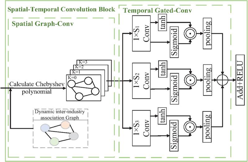
Figure 4 Structure of the spatial-temporal graph convolution block.
(1) Spatial Graph Convolution
Spatial Graph Convolution employs Chebyshev polynomial expansion to approximate spectral graph convolution, enabling each industry node to perceive multi-level relational dependencies through the design of higher-order polynomials. Unlike the fixed weight assignment in static graph convolution, this approach dynamically binds the spatial attention weights with each polynomial term, thereby establishing a dynamically coupled mechanism for inter-industry associations.
| (3) |
where represents the approximate convolution kernel; represents the graph convolution operation; represents the input; represents the polynomial coefficients iteratively updated during training; represents the -th order Chebyshev polynomial, with the input being the normalized Laplacian matrix.
(2) Temporal Gated Convolution
Temporal Gated Convolution captures complex temporal patterns through a multi-scale gated residual architecture. The model parallelly deploys three groups of GTU units with different scales. The small-scale convolution focuses on extracting short-term fluctuation features, the medium-scale captures regular fluctuations induced by periodicity, and the large-scale models global trend features across time periods. After dimensionality reduction via max pooling, the outputs from all scales are fused with the original input through residual connections, preserving feature information at multiple time granularities while avoiding the vanishing gradient problem.
| (4) |
where adopts a dynamic pooling strategy based on attention weights, prioritizing the preservation of key time-step features; represents convolution kernels of different scales, and represents the input.
2.2.2 Limitations analysis
Although the DSTAGNN model architecture captures the correlation features of power load, there are still two limitations in the industry power load forecasting scenario:
1. Single Representation of Temporal Features: The existing DSTAGNN model does not model temporal features separately, but rather extracts temporal information through the time attention mechanism and time-gated convolution. However, the time attention mechanism is prone to noise interference when dealing with long time series, leading to decreased attention on key time steps and affecting the capture of long-term dependencies. Although the time-gated convolution can extract local temporal features, due to the fixed size of the convolution kernel, it is difficult to adapt to load change patterns at different time scales. Therefore, a more flexible temporal feature modeling method is needed to achieve comprehensive representation of temporal features.
2. Lack of Dynamic Inter-industry Association Graph Construction Method: In the industrial load forecasting field, traditional graph-based modeling methods are usually based on geographical proximity to build spatial association models. However, industrial loads and regional power loads have essential differences: the former does not have geographical clustering features but forms a complex association network through economic links such as industrial chains and supply-demand relationships. This characteristic makes traditional graph models based on geographical distance unable to accurately represent the interaction mechanisms between industries. It is necessary to break through the limitations of spatial proximity assumptions and construct dynamic graphs based on economic correlations between industries, enabling dynamic inter-industry association modeling.

Figure 5 Architecture diagram of the Time2Vector block.
2.3 Time2Vector Block
To address the issue of single representation of temporal features, the Time2Vector block [27] is introduced to learn both periodic and non-periodic features by mapping time information into multidimensional vectors and adaptively capturing different pattern modes in the time series. As shown in Figure 5 and Equation (5), this time encoding function adopts a piecewise design to achieve multi-scale temporal feature extraction: when the dimension index is , it captures the long-term trend components of the time series; when is used, it maps the data through a nonlinear function to analyze multi-periodic features. The final output vector encodes the time scalar into a time feature with physical significance, providing a time vector for the downstream spatiotemporal graph convolution.
| (5) |
where is the learnable frequency parameter, which controls the period length of the time features; is the learnable phase parameter, which adjusts the offset of the time waveform; uses the sin and cos functions to capture periodicity.
2.4 DIAG Construction Based on VECM
2.4.1 VECM
To address the challenge of economic association modeling in industrial electricity load forecasting, this paper introduces the VECM [28] to construct the DIAG. This model breaks through the traditional spatial proximity assumption by analyzing the dynamic interaction patterns of electricity loads between industries through cointegration tests and error correction mechanisms.
The basic form of VECM is as follows: Assume there is a time series vector , where each component represents a time series. In analyzing the electricity load association mechanism between industries, these time series correspond to the load sequence of the -th industry. By performing linear regression on , the (Vector Autoregressive Model) VAR model can be obtained, and its expression is:
| (6) |
where represents the model variables; represents the -lagged values of the model variables; is the parameter matrix; and is the random disturbance term. By performing a differencing transformation on Equation (6), the general expression of VECM is obtained:
| (7) |
where Matrix is the adjustment coefficient matrix, with each column vector representing the weights of a cointegration combination, reflecting the response when the long-term equilibrium relationship between variables deviates. Matrix is the cointegration vector matrix, where each row vector corresponds to a cointegration vector, and the error correction term represents the long-term equilibrium relationship between the variables. Meanwhile, the coefficient matrix of the independent variable differenced terms indicates the impact of the short-term fluctuations of the variables on the short-term changes of the dependent variable [29].
2.4.2 Variance decomposition method
Based on the above analysis, the coupling and association characteristics between industries are mainly influenced by parameters . In the VECM model, the variance decomposition method is commonly used to reorganize information and extract key insights from these three parameters. The variance decomposition method decomposes the total fluctuation of a complex variable (i.e., its variance) into contributions from its components, thereby quantitatively measuring the impact of different factors on the overall fluctuation.
By transforming Equation (7) into the VAR model and introducing the lag operator , that is:
| (8) |
where represents the -th order lag operator, and represents the identity matrix.
If the model corresponding to Equation (8) is stationary, it can be represented as an infinite moving average process of a white noise vector, that is:
| (9) |
where represents the coefficient matrix, indicating the influence of the -th order lag white noise vector on , and .
The component form corresponding to Equation (9) is as follows:
| (10) |
In the equation, represents the specific elements of the coefficient matrix , meaning the influence of the -th component of the -th order lag disturbance vector on .
Under the assumption that the components of are uncorrelated and the covariance matrix is a diagonal matrix, the variance of is as follows:
| (11) |
where represents the variance of the -th variable.
The variance of can be decomposed into uncorrelated components. By observing the relative contribution rate of the variance of variable based on the shock to the variance of , we can assess the impact of the -th variable on the -th variable. In other words, by calculating the size of , we can perform a quantitative analysis of the coupling and associative characteristics between industries. The formula for calculating is as follows:
| (12) |
Based on the above explanation of the basic structure and mathematical significance of the VECM model, the steps for constructing the DIAG using the VECM model are shown in Figure 6:
(1) Perform the Augmented Dickey-Fuller (ADF) test on industrial load series. If there are non-stationary series, use the differencing method to eliminate trend and seasonal fluctuations [30], thus addressing the spurious regression problem caused by non-stationary series, reducing the risk of misjudging false associations between industries.

Figure 6 Flowchart of constructing DIAG based on VECM.
(2) Construct the VAR model framework, select the optimal lag order based on Akaike Information Criterion (AIC), Schwarz Information Criterion (SIC), and Hannan-Quinn (HQ) criteria, capture the transmission delays of industry impacts, and use the Johansen cointegration test to analyze the long-term equilibrium relationships between industries.
(3) Build the VECM model based on the cointegration results. This model captures the adjustment mechanism of the long-term relationships between industries through the error correction term (ECT), and also quantifies the short-term mutual influence of industrial load changes by incorporating short-term fluctuation terms.
(4) Use the variance decomposition method to calculate the contribution of each industry to the load fluctuations of other industries, resulting in a contribution matrix between industries. Normalize it into an adjacency matrix weight, and use it to measure the correlation between nodes. Then, perform binarization to set non-zero elements to 1, generating the graph structure. This process ensures that in graph convolution operations, each node only aggregates the most relevant neighbor information.
(5) In summary, form DIAG, which reflects the interaction of industrial power loads over time. As time progresses, the edge weights in the graph will be continuously adjusted based on the time-varying association strengths between industrial loads, capturing the dynamic changes in industrial load fluctuations.
3 Industry Association Dynamic Graph Neural Network Model Integrating Periodic Features
The structure of the IADGNN model integrating periodic features is shown in Figure 7. This model consists of the Time2Vector block, DIAG constructed based on VECM, and IADGNN model. The overall method flow is shown in Figure 8. and is detailed as follows:
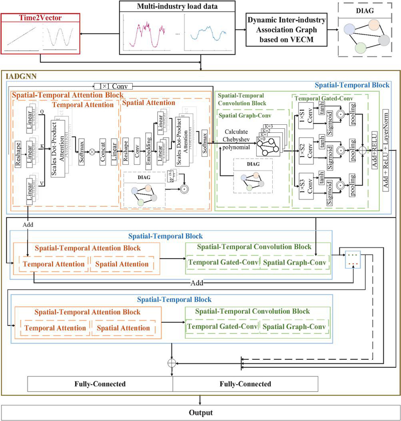
Figure 7 Overall architecture diagram.

Figure 8 Overall flowcharts.
First, the sliding window method is used to divide the normalized industrial load data into training, validation, and test sets.
Next, the Time2Vector time embedding layer is used to extract the periodic and non-periodic features of the data, which are then used as input along with the original data.
Subsequently, the IADGNN model is employed for prediction. The model is composed of multiple spatial-temporal blocks stacked together. Each block includes two main components: the dynamic spatial-temporal attention block and spatial-temporal graph convolution block, which are used to fully extract and integrate the spatial-temporal features from multi-dimensional load data. Specifically, the dynamic spatial-temporal attention block includes a temporal attention layer and a spatial attention layer. The temporal attention layer captures dependencies between different time steps in the load sequence, enhancing the model’s ability to perceive temporal dynamics. The spatial attention layer, based on the DIAG, learns the correlation between different industry nodes adaptively, capturing the time-varying industry association strength and guiding the more efficient propagation of information in the graph.
In the spatial-temporal graph convolution block, the spatial graph convolution part uses DIAG to replace the static adjacency matrix, modeling the local structure of industry nodes and further enhancing the model’s ability to model the dynamic structure of industries. The temporal gated convolution models the feature changes of nodes over time using a gating mechanism, effectively mitigating the issue of information attenuation in long sequence learning. Multiple spatial-temporal blocks are stacked sequentially, and the output of each block is passed to the next layer for deeper feature extraction.
Finally, after all the spatial-temporal blocks, the model uses a fully connected layer to map the multi-layer integrated features to the final prediction space. A batch inverse normalization is applied at the output end to restore the data to the original load scale, and the final prediction result is output.
4 Test Cases
4.1 Selection of Industrial Load Data
The data used in this study initially consist of electricity load data from eleven different industries in a province of China, covering the period from January 1, 2022, to December 31, 2022, with a time interval of 15 minutes, resulting in 96 data points per day. Given the significant correlations among electricity loads across different industries, Pearson’s correlation coefficient, which measures the linear correlation between two variables and ranges from 1 to 1, is employed to quantify the inter-industry load relationships, where values closer to 1 indicate stronger positive correlations. To reduce the influence of irrelevant or noisy industries and improve model performance, a subset of industries with high correlation levels is selected from the original eleven industries and used as inputs to the IADGNN model. The correlation analysis results are presented in Table 1. Industries with a Pearson correlation coefficient greater than or equal to 0.8 are selected for experimental analysis, resulting in four representative industries: transportation, storage and postal services; information transmission, software and information technology services; wholesale and retail; and leasing and business services.
Table 1 Average Cross-industry correlation table
| The Average Correlation | |
| Industry | with Other Industries |
| Information transmission, software and information technology services | 0.82 |
| Leasing and business services industry | 0.82 |
| Transportation, warehousing and postal industry | 0.8 |
| Wholesale and retail trade | 0.8 |
| Finance industry | 0.79 |
| Real estate industry | 0.79 |
| Construction industry | 0.78 |
| Public services and management organizations | 0.76 |
| Accommodation and cateringindustry | 0.75 |
| Agriculture, forestry, animal husbandry and fisheries | 0.43 |
| Industrial | 0.3 |
4.2 Construction of the DIAG
Based on the construction process shown in Figure 6. of Section 2.4, the following steps are implemented sequentially:Perform the ADF test on the data [31]. The test results are shown in Table 2. As can be seen from Table 2, the station and cluster power series all passed the stationarity test with a result of “Yes,” indicating that these power series are stationary and do not require differencing for subsequent steps.
Table 2 Stationarity test results of power series
| Variable | ADF Statistic | p-value | Is Stationary |
| Transportation, warehousing and postal industry | 39.37894127 | 0 | Yes |
| Information transmission, software and information technology services | 48.9270821 | 0 | Yes |
| Wholesale and retail trade | 49.87655251 | 0 | Yes |
| Leasing and business services industry | 55.50486399 | 0 | Yes |
Establish a general VAR model based on Equation (6), and determine the optimal lag order of the model as 197 using the AIC, SIC, and HQ criteria. The Johansen cointegration test is then applied to the power series, and the test results are shown in Table 3. As observed from Table 3, there exists a cointegration relationship among the data, which satisfies the basic requirement for constructing the VECM model. Therefore, the model can be built.
Table 3 Trace statistic test results
| Assuming the Number of Cointegration Equations | Trace Statistic | 5% Critical |
| None | 1058.041848 | 55.2459 |
| At most 1 | 732.6513914 | 35.0116 |
| At most 2 | 457.7680272 | 18.3985 |
| At most 3 | 194.4727844 | 3.8415 |
Table 4 Maximum eigenvalue test results
| Assuming the Number of | Maximum | |
| Cointegration Equations | Eigenvalue Statistic | 5% Critical |
| None | 325.3904566 | 30.8151 |
| At most 1 | 274.8833642 | 24.2522 |
| At most 2 | 263.2952428 | 17.1481 |
| At most 3 | 194.4727844 | 3.8415 |
As shown in Tables 3 and 4, both the Trace statistic test and the Maximum Eigenvalue test indicate that there are three cointegrating relationships among the load series of the four industries, which satisfies the basic condition for constructing the VECM. Accordingly, the VECM model is built based on Equation (7).
Following the above analysis and the theoretical framework in Section 1.4.2, variance decomposition is performed on the error terms of the constructed VECM. The variance decomposition results for the transportation, storage and postal services industry; information transmission, software and information technology services industry; wholesale and retail industry; and leasing and business services industry are shown in Figure 9. The specific analysis is as follows:
(1) Transportation, Storage and Postal Services: Variance decomposition results show that fluctuations in this industry are primarily driven by its own historical factors, with an initial contribution of 99.1%, gradually decreasing to about 74% in the long term. Among other industries, the contribution of the wholesale and retail industry increases significantly over time, from 0.4% to 13.5%, becoming the most influential external factor. The contribution of leasing and business services rises from 0.26% to 7.3%, ranking second, while the information technology industry contributes relatively little but gradually increases from 0.2% to 5.2%.

Figure 9 Variance decomposition results of the four industries.
(2) Information Transmission, Software and IT Services: This industry is initially highly influenced by its own factors. However, over time, the contribution from the leasing and business services industry rises sharply from 1.96% to 31.1%, becoming the main external driving force. The contribution from wholesale and retail increases slightly from 0.2% to 3.5%, while transportation’s contribution remains below 0.2% throughout.
(3) Wholesale and Retail: This industry has a high self-contribution that gradually declines. Among external contributors, leasing and business services have the most notable impact, increasing from 0.05% to 9.9%. The contribution from the information industry stabilizes after dropping from 5.1% to 3.5%, while the transportation industry’s contribution remains below 2.8%. In the long term, the explanatory power of leasing and business services on its fluctuations significantly increases, especially in the later stages, becoming the dominant external factor.
(4) Leasing and Business Services: This industry’s own contribution remains dominant in the long term, though the contribution from wholesale and retail declines from 30.9% to 21.4%, still representing a major external source. The contribution from the information industry steadily increases from 9.5% to 16.5%, while transportation’s contribution rises from 0.7% to 3.7%. Together, they drive the fluctuations in this industry. Overall, the marginal influence of the information and transportation industries is expanding, while the contribution from wholesale and retail shows a decreasing trend.
4.3 Industrial Load Forecasting Based on the Time2Vector-IADGNN Model
In this study, a sliding window approach is used to divide the normalized industrial load data into training, validation, and test sets in a ratio of 6:2:2, with both the input and prediction step lengths set to 96. Based on the training set, the Time2Vector-IADGNN model is trained using mean squared error (MSE) as the loss function and the Adam optimizer for gradient descent. Hyperparameter tuning is conducted using the validation set.
To prevent overfitting, early stopping is introduced, and a maximum number of training epochs is set. Additionally, a dynamic learning rate adjustment strategy is applied to stabilize training fluctuations and enhance both convergence and generalization performance. After training, the final model is used to predict industrial loads on the test set and outputs the corresponding forecast results.
In this study, three evaluation metrics are used to assess the forecasting performance: mean absolute error (MAE), root mean square error (RMSE), and mean absolute percentage error (MAPE) [32]. The calculation formulas for these metrics are provided in Equations (13)–(15).
| (13) | ||
| (14) | ||
| (15) |
where represents the number of prediction samples; denotes the predicted values; denotes the actual values.
4.4 Comparative Empirical Studies
To evaluate the prediction accuracy of the proposed method, we compare it with the following prediction methods:
BiLSTM-Attention (Single Industry): Uses the BiLSTM-Attention model to predict the load of each industry individually, and then aggregates the predictions to obtain the final results for all industries.
BiLSTM-Attention (Multi-Industry): Uses the BiLSTM-Attention model to predict the loads of all industries simultaneously with multi-input and multi-output.
STGCN [33] (Spatio-Temporal Graph Convolutional Networks): Uses the STGCN model for multi-input and multi-output prediction of the loads across all industries.
STAGNN (Spatial-Temporal Aware Graph Neural Network): Uses the STAGNN model for multi-input and multi-output prediction of the loads across all industries.
The specific hyperparameters used in the experiments are listed in Table 5.
Table 5 Optimal parameter conffgurations for different models
| Models | Optimal Configurations |
| BiLSTM-Attention (Single Industry) | hidden_size=256, number of units in the Attention layer=256, batch_size=32, learning rate=0.01 |
| BiLSTM-Attention (Multi-Industry) | hidden_size=156, number of units in the Attention layer=156, batch_size=96, learning rate=0.01 |
| STGCN | Number of Spatio-temporal Convolution block=4, the channels of Temporal Convolution Layer=64, the channels of Spatial Convolution Layer=16, Temporal Convolution Kernel Size=3, Spatial Convolution Kernel Size=3, batch_size=128, learning rate=0.001 |
| STAGNN | Number of Spatial-Temporal block=4, Number of Attention Heads in Temporal Attention block=3, Number of Attention Heads in Spatial Attention block=3, Number of Channels in Spatial Graph Convolution Layer=32, Number of Channels in Temporal Gated Convolution Layer=32, Temporal Gated Convolution Kernel Size=9, 15, 21, batch_size=64, learning rate=0.0001 |
| Time2vetor-IADGNN | Number of Spatial-Temporal block=4, Number of Attention Heads in Temporal Attention block=3, Number of Attention Heads in Spatial Attention block=3, Number of Channels in Spatial Graph Convolution Layer=32, Number of Channels in Temporal Gated Convolution Layer=32, Temporal Gated Convolution Kernel Size=9, 15, 21, batch_size=64, learning rate=0.0001 |
The comparative results are shown in Table 6 and Figure 10. The proposed model outperforms all benchmark methods across all evaluation metrics. Experimental results demonstrate that in the load forecasting task for four industries, the Time2Vector-IADGNN model achieves average improvements of 42.72%, 44.03%, and 37.98% over the BiLSTM-Attention (Single Industry) model across the three evaluation metrics. This is mainly because the BiLSTM-Attention model primarily relies on long-term dependency modeling in time series. Although it can effectively capture nonlinear temporal features, it lacks the capability to model the dynamic inter-industry correlations in load data.
Compared to the BiLSTM-Attention (Multi-Industry) model, Time2Vector-IADGNN improves prediction performance by an average of 42.96%, 44.44%, and 39.26% across the three evaluation metrics. This is because the BiLSTM-Attention model, when applied to industrial data, still focuses mainly on the temporal prediction of individual industrial data and fails to effectively leverage the complex dynamic relationships between industries.
Table 6 Comparison of evaluation metrics for different models
| BiLSTM- | BiLSTM- | |||||
| Attention | Attention | |||||
| (Single | (Multi- | Time2Vector- | ||||
| Industry) | Industry) | STGCN | STAGNN | IADGNN | ||
| Transportation, | RMSE(MW) | 6.90 | 7.38 | 7.81 | 6.62 | 5.03 |
| warehousing and | MAE(MW) | 5.54 | 5.90 | 6.31 | 5.22 | 3.87 |
| postal industry | MAPE(%) | 4.37 | 4.62 | 5.49 | 4.22 | 3.08 |
| Information | RMSE(MW) | 3.49 | 3.10 | 3.41 | 3.29 | 1.85 |
| transmission, | MAE(MW) | 2.94 | 2.55 | 2.71 | 2.87 | 1.44 |
| software and | MAPE(%) | 2.09 | 1.82 | 1.98 | 2.08 | 1.05 |
| information | ||||||
| technology | ||||||
| services | ||||||
| Wholesale and | RMSE(MW) | 15.57 | 16.19 | 11.62 | 10.56 | 8.37 |
| retail trade | MAE(MW) | 12.22 | 13.15 | 9.19 | 8.45 | 6.72 |
| MAPE(%) | 4.61 | 5.26 | 4.00 | 3.59 | 3.07 | |
| Leasing and | RMSE(MW) | 6.19 | 6.29 | 5.91 | 5.66 | 3.07 |
| business | MAE(MW) | 5.21 | 5.32 | 4.46 | 4.88 | 2.61 |
| services | MAPE(%) | 7.74 | 7.84 | 7.62 | 7.74 | 4.73 |
| industry |
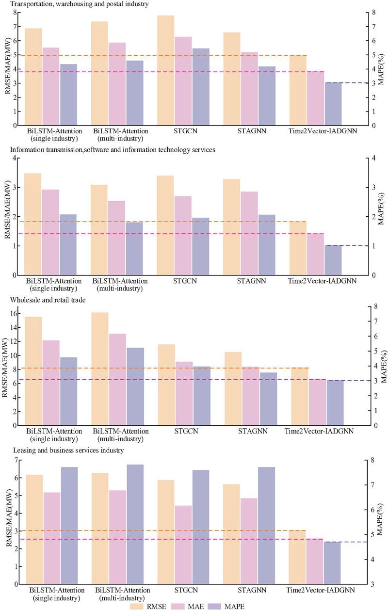
Figure 10 Comparison of evaluation metrics for different models.
Against the STGCN model, Time2Vector-IADGNN achieves improvements of 39.36%, 38.53%, and 38.08%, while improvements over the STAGNN model are 33.58%, 35.71%, and 32.55% across the respective evaluation metrics. Both STGCN and STAGNN adopt static graph structures to model spatio-temporal information. While they can extract spatio-temporal features of load data using graph neural networks, their modeling capabilities are constrained by the limitations of static graphs, making it difficult to capture the dynamic evolution of inter-industry relationships.
In contrast, Time2Vector-IADGNN enhances temporal feature representation through the introduction of Time2Vector, and constructs dynamic relational graphs using the Vector Error Correction Model (VECM), enabling the model to capture both long-term equilibrium and short-term dynamic fluctuations within industries. Additionally, the DIAG of IADGNN allows the model to more accurately learn inter-industry associations, resulting in superior forecasting performance in industrial load prediction scenarios.
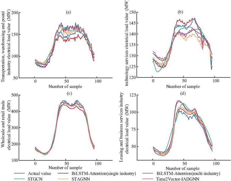
Figure 11 Comparison of prediction results from different models.
To further visualize the comparison, four groups of results were randomly selected from the test sets of the four industries, with each group containing 96 data samples, as shown in Figure 11, the prediction curves of different models exhibit noticeable differences in their relative positions and deviation directions. In Figure 11(a), the prediction curves of the compared models gradually diverge during the load rising stage, with some models showing overall underestimation or overestimation, whereas the Time2Vector-IADGNN model maintains a relatively close alignment with the true load throughout the entire prediction interval. In the sample illustrated in Figure 11(b), the prediction discrepancies among different models are further amplified in the high-load region, leading to a more dispersed distribution of the predicted curves. In contrast, the predictions of the Time2Vector-IADGNN model show smaller relative deviations from the true load and do not exhibit evident systematic bias. As shown in Figure 11(c), although most models are able to capture the overall load variation pattern, some models present persistent deviations during the descending stage, while the Time2Vector-IADGNN model is able to maintain a more stable relative tracking relationship. For Figure 11(d), different models display varying deviation directions over the entire prediction horizon, whereas the prediction curve of the Time2Vector-IADGNN model remains highly consistent with the true load across different stages. Overall, the Time2Vector-IADGNN model is capable of effectively reducing prediction deviations and maintaining reasonable relative positions of the predicted curves at different stages, thereby demonstrating superior overall predictive performance in multi-model comparisons.
4.5 Ablation Empirical Studies
While the comparative experiments validated the overall performance of the proposed model, they did not evaluate the contributions of individual components, making it difficult to determine their importance. Therefore, an ablation study was conducted to further assess the effectiveness of each component. Models were constructed by systematically removing individual components from the proposed architecture, and their performance on the dataset was analyzed in terms of various evaluation metrics. As shown in Table 7 and Figure 12, the experimental models include: GNN (without Time2Vector and DIAG), Time2Vector-GNN (without DIAG), IADGNN (without Time2Vector), and Time2Vector-IADGNN. All models were trained with the same hyperparameter settings as those used for Time2Vector-IADGNN in Table 4. The results indicate that removing either the Time2Vector block or the DIAG component based on VECM leads to a decline in prediction accuracy. The combination of both blocks yields the best performance across all industries. A detailed analysis is provided below:
(1) Time2Vector
Table 7 Comparison of evaluation metrics for ablation experiments
| GNN | Time2Vector- | ||||
| (No | GNN | IADGNN | |||
| Time2Vector, | (No | (No | IADGNN- | ||
| DIAG) | DIAG) | Time2Vector) | Time2Vector | ||
| Transportation, | RMSE (MW) | 6.17 | 5.54 | 5.45 | 5.03 |
| warehousing | MAE (MW) | 4.83 | 4.30 | 4.40 | 3.87 |
| and postal | MAPE (%) | 3.89 | 3.40 | 3.70 | 3.08 |
| industry | |||||
| Information | RMSE (MW) | 3.08 | 2.24 | 2.13 | 1.85 |
| transmission, | MAE (MW) | 2.57 | 1.76 | 1.78 | 1.44 |
| software | |||||
| and information | MAPE (%) | 1.82 | 1.25 | 1.29 | 1.05 |
| technology | |||||
| services | |||||
| Wholesale | RMSE (MW) | 10.28 | 8.55 | 9.49 | 8.37 |
| and retail | MAE (MW) | 8.07 | 6.99 | 7.50 | 6.72 |
| trade | MAPE (%) | 3.40 | 3.12 | 3.32 | 3.07 |
| Leasing | RMSE (MW) | 3.97 | 3.66 | 3.52 | 3.07 |
| and business | MAE (MW) | 3.49 | 3.16 | 2.88 | 2.61 |
| services industry | MAPE (%) | 6.49 | 5.78 | 5.00 | 4.73 |

Figure 12 Comparison of evaluation metrics for ablation experiments.
The results show that Time2Vector-IADGNN outperforms IADGNN (no Time2Vector) across all industrial datasets, with average improvements of 11.37%, 12.72%, and 12.29% across the three evaluation metrics. Similarly, Time2Vector-GNN surpasses GNN by 15.51%, 16.31%, and 15.81%, respectively. This improvement is attributed to the fact that, in the absence of Time2Vector, the model relies solely on linear extrapolation from historical load values and cannot fully exploit temporal information. With the introduction of Time2Vector, a trainable time embedding mechanism maps temporal features into a high-dimensional space, allowing the model to adaptively learn the temporal influence patterns on load variation. This enables the model to capture both non-periodic and periodic patterns in the data, thereby enhancing its ability to represent temporal features and improving forecasting accuracy.
(2) DIAG Construction Based on VECM
The results further show that Time2Vector-IADGNN outperforms Time2Vector-GNN across all industrial datasets, with average improvements of 11.29%, 12.35%, and 11.37% in the three evaluation metrics. Likewise, IADGNN outperforms GNN by 15.44%, 16.03%, and 14.74%, respectively. Without the DIAG constructed using VECM, the model relies solely on static inter-industry relationships or raw time-series features, which are inadequate for modeling the complex and evolving relationships among industries. In contrast, the DIAG constructed with VECM effectively captures long-term equilibrium relationships and short-term dynamic interactions among industries. By leveraging cointegration relationships, it uncovers deeper inter-industry linkages, thereby improving the model’s ability to describe dynamic dependencies and enhancing the accuracy of load forecasting.
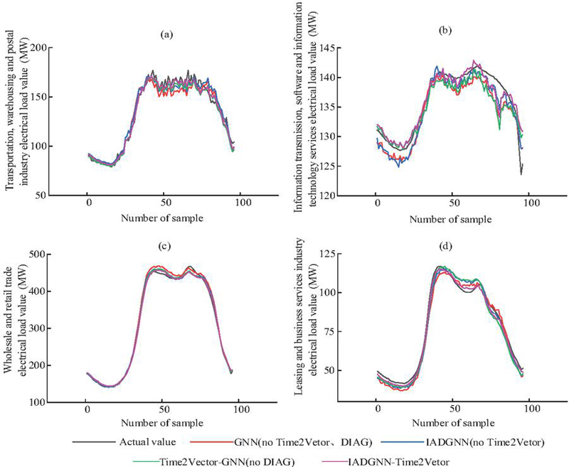
Figure 13 Comparison of prediction results for ablation experiments.
In conclusion, each component plays a critical role in the forecasting task and contributes to the overall performance through synergistic effects. Time2Vector enhances the model’s ability to represent temporal characteristics of load data, enabling more accurate modeling of temporal patterns. The VECM-based DIAG further strengthens the model’s capability to capture complex inter-industry relationships, especially the long-term equilibrium and short-term fluctuation mechanisms. Ultimately, Time2Vector-IADGNN integrates the advantages of both blocks and achieves the best forecasting performance across all industrial datasets, with average improvements of 24.97%, 26.42%, and 25.08% over the baseline GNN model across the three evaluation metrics.
To further visualize the comparison, four groups of results were randomly selected from the test sets of the four industries, with each group containing 96 data samples, as shown in Figure 13, the temporal load patterns vary across different industries. Specifically, the loads in Figures 13(a) and 13(b) exhibit relatively complex fluctuations, with pronounced variations over time, whereas the loads in Figures 13(c) and 13(d) are comparatively smoother, showing clearer overall trends. Under these different load characteristics, the proposed IADGNN-Time2Vector model is able to effectively track the overall evolution of the true load in all subfigures, with the predicted curves maintaining a high degree of consistency with the actual values. In contrast, the other benchmark models exhibit certain deviations in some samples, particularly in scenarios with more complex load fluctuations, where the stability of the prediction results is relatively insufficient. Therefore, the proposed IADGNN-Time2Vector model demonstrates strong adaptability to different load fluctuation characteristics and is capable of maintaining stable predictive performance across multi-industry scenarios involving both complex variations and smooth trends, which further validates its effectiveness in multi-industry load forecasting tasks.
5 Conclusion
To address the challenges of modeling complex temporal patterns and inter-industry associations in industrial load forecasting, this study proposes a Time2Vector-IADGNN-based prediction model. The model is validated on a provincial-level industrial electricity load dataset from China, highlighting its advantages in forecasting accuracy. The main conclusions are as follows:
The Time2Vector block achieves adaptive learning of dynamic periodicity and high-dimensional embedding for load data through nonlinear time-series feature mapping, effectively compensating for the lack of time feature representation. After introducing Time2Vector, the overall prediction performance improves by an average of 14.00%, significantly outperforming models without time embedding.
The VECM-based DIAG reveals the long-term correlation and short-term fluctuation effects of industrial loads in the time evolution process. After incorporating the DIAG, the overall prediction performance improves by an average of 13.54%, significantly outperforming traditional graph structure models.
IADGNN dynamically captures the evolving inter-industry correlations driven by temporal and load fluctuations through the DIAG structure, effectively modeling the complex and time-varying load dependencies among industries. Compared to traditional models and static graph models, the proposed model achieves an average improvement of 39.10% in overall prediction performance, demonstrating its advantages in industrial load forecasting.
References
1. Ahmad T, Zhang D. A critical review of comparative global historical energy consumption and future demand: The story told so far. Energy Reports, 2020, 6: 1973–1991.
2. Xu, C, Liu, J, Chen, L, Zhang, P, and He, W (2025). Advanced Machine Learning Solutions for Power Load Forecasting and Power Grid Planning Optimization. Distributed Generation & Alternative Energy Journal, 40(2), 259–278.
3. Hepburn C, Qi Y, Stern N, et al. Towards carbon neutrality and China’s 14th Five-Year Plan: Clean energy transition, sustainable urban development, and investment priorities. Environmental Science and Ecotechnology, 2021, 8: 100130.
4. Gang L I, Hong F, Yunpeng L I U. Large-model drive technology in new power system: status, challenges and prospects. High Voltage Engineering, 2024, 50(7): 2864–2878.
5. Habbak H, Mahmoud M, Metwally K, et al. Load forecasting techniques and their applications in smart grids. Energies, 2023, 16(3): 1480.
6. Han F J, Wang X H, Qiao J, et al. Review on artificial intelligence based load forecasting research for the new-type power system. Proc. CSEE, 2023, 43(22): 8569–8591.
7. Hongtao L, Shuo L, Junwei D U, et al. Review of deep learning applied to time series prediction. Journal of Frontiers of Computer Science & Technology, 2023, 17(6): 1285.
8. Unlu A, Peña M, Wang Z. Comparison of the combined deep learning methods for load forecasting. 2023 IEEE Power & Energy Society Innovative Smart Grid Technologies Conference (ISGT). IEEE, 2023: 1–5.
9. Buratto W G, Muniz R N, Nied A, et al. Seq2Seq-LSTM with attention for electricity load forecasting in Brazil. IEEE Access, 2024, 12: 30020–30029.
10. Ma G, Hu S, Pang N and Zhou Q. Strategy Improved Pelican Algorithm Optimization ELM for Short-Term Electricity Load Forecasting. Distributed Generation & Alternative Energy Journal, 2025, 40, 85–108.
11. Yong B, Huang L, Li F, et al. A research of Monte Carlo optimized neural network for electricity load forecast. The Journal of Supercomputing, 2020, 76: 6330–6343.
12. Alkayal S, Almisbahi H, Baowidan S, Alkayal E. Air Pollution Trends and Predictive Modeling for Three Cities with Different Characteristics Using Sentinel-5 Satellite Data and Deep Learning. Atmosphere. 2025; 16(2):211.
13. Hu Y, Li J, Hong M, et al. Industrial artificial intelligence based energy management system: Integrated framework for electricity load forecasting and fault prediction. Energy, 2022, 244.
14. Kartini U T, Ardyansyah D P, Yundra E. Hybrid Model For The Next Hourly Electricity Load Demand Forecasting Based on Clustering and Weather Data. 2020.
15. Tan M, Yuan S, Li S, et al. Ultra-short-term industrial power demand forecasting using LSTM based hybrid ensemble learning. IEEE transactions on power systems, 2019, 35(4): 2937–2948.
16. Wang Y, Chen J, Chen X, et al. Short-term load forecasting for industrial customers based on TCN-LightGBM. IEEE Transactions on Power Systems, 2020, 36(3): 1984–1997.
17. Bessani M, Massignan J A D, Santos T M O, et al. Multiple households very short-term load forecasting using bayesian networks. Electric Power Systems Research, 2020, 189: 106733.
18. Kychkin A V, Chasparis G C. Feature and model selection for day-ahead electricity-load forecasting in residential buildings. Energy and Buildings, 2021, 249: 111200.
19. Alikhani P, Tjernberg L B, Astner L, et al. Forecasting the electrical demand at the port of Gävle Container termina. 2021 IEEE PES Innovative Smart Grid Technologies Europe (ISGT Europe). IEEE, 2021: 1–6.
20. Yadav K, Singh M. A novel energy management of public charging stations using attention-based deep learning model. Electric Power Systems Research, 2025, 238.
21. Fan G. Research and implementation on parallel power load prediction[D]. North China Electric Power University (Beijing), 2022.
22. Guo Y, Li Y, Qiao X, et al. BiLSTM multitask learning-based combined load forecasting considering the loads coupling relationship for multienergy system. IEEE Transactions on Smart Grid, 2022, 13(5): 3481–3492.
23. He Z, Zhao C, Huang Y. Multivariate time series deep spatiotemporal forecasting with graph neural network. Applied Sciences, 2022, 12(11): 5731.
24. Lv Y, Wang L, Long D, et al. Multi-area short-term load forecasting based on spatiotemporal graph neural network. Engineering Applications of Artificial Intelligence, 2024, 138.
25. Wang Y, Rui L, Ma J, et al. A short-term residential load forecasting scheme based on the multiple correlation-temporal graph neural networks. Applied Soft Computing, 2023, 146(000):12.
26. Lan S, Ma Y, Huang W, et al. Dstagnn: Dynamic spatial-temporal aware graph neural network for traffic flow forecasting. International conference on machine learning. PMLR, 2022: 11906–11917.
27. Kazemi S M, Goel R, Eghbali S, et al. Time2Vec: Learning a Vector Representation of Time. 2019.
28. Liu Y, Zhao X, Lu D, et al. Impact of policy incentives on the adoption of electric vehicle in China. Transportation research part A: policy and practice, 2023, 176: 103801.
29. Ren X, Shao Q, Zhong R. Nexus between green finance, non-fossil energy use, and carbon intensity: Empirical evidence from China based on a vector error correction model. Journal of Cleaner Production, 2020, 277: 122844.
30. Song W, Zhang X. Research on the linkage between lithium carbonate futures market and spot market: Based on the perspective of VECM model. Northern Economics and Trade, 2025, (2): 93–98.
31. Ma G, Hu S, Pang N, et al. Strategy Improved Pelican Algorithm Optimization ELM for Short-Term Electricity Load Forecasting. Distributed Generation & Alternative Energy Journal, 2025, 40(1), 85–108.
32. Chen H, Meng L, Xi Y, et al. GRU Based Time Series Forecast of Oil Temperature in Power Transformer. Distributed Generation & Alternative Energy Journal, 2023, 38(2), 393–412.
33. Yu B, Yin H, Zhu Z. Spatio-temporal graph convolutional networks: A deep learning framework for traffic forecasting. arXiv preprint arXiv:1709.04875, 2017.
Biographies

Bo Zhao received the B.S. and M.S. degree from Beihang University, Beijing, China, in 2000 and 2003, respectively, and the Ph.D degree from China Electric Power Research Institute, Beijing, China, in 2013. He was a Professor-level senior engineer with China Electric Power Research Institute, Beijing, China. He is currently a researcher with the School of Automation, Beijing Information Science and Technology University, Beijing, China. His main research interests include new energy and energy storage and intelligent power distribution and consumption technology.

Ying Zheng received the B.S. degree in engineering from Beijing Information Science and Technology University, Beijing, China, in 2023. She is currently pursing the M.S. degree with the School of Automation, Beijing Information Science and Technology University, Beijing, China. Her main research interests are power system load analysis and forecasting.

Ying Hao received the B.S. degree from Hebei University of Science and Technology, Shijiazhuang, China, in 2008, the M.S. and Ph.D degree from Beijing Institute Of Technology, Beijing, China, in 2010 and 2020, respectively. She is currently an Associate Professor with the School of Automation, Beijing Information Science and Technology University. Her main research interests include new energy power generation and multi-energy synergy technology.

Xin Li received the B.S. degree in engineering from Beijing Information Science and Technology University, Beijing, China, in 2023. She is currently pursing the M.S. degree with the School of Automation, Beijing Information Science and Technology University, Beijing, China. Her main research interests are photovoltaic power prediction.

Jiaheng Yang received the B.S. degree from Nanjing University of Posts and Telecommunications, Nanjing, China, in 2024. He is currently pursing the M.S. degree with the School of Automation, Beijing Information Science and Technology University, Beijing, China. His main research interest is about renewable energy generation and power system load forecasting.
Distributed Generation & Alternative Energy Journal, Vol. 41_3, 753–790
doi: 10.13052/dgaej2156-3306.4139
© 2026 River Publishers