Multi-Objective Scheduling of V2G-Enabled PEVs in Local Multi-Energy Systems: Balancing Profitability and Carbon Emissions Using Time-Varying Operational Profiles
Yan Hou1,* and Shuling Yang2
1School of Economics, Management and Law, Jilin Normal University, Siping 136000, Jilin, China
2School of Foreign Languages, Jilin Normal University, Siping 136000, Jilin, China
E-mail: houyan@jlnu.edu.cn; yangshuling@jlnu.edu.cn
*Corresponding Author
Received 15 October 2025; Accepted 25 April 2026
Abstract
Plug-in electric vehicles (EVs) introduce both benefits and challenges to effective energy regulation when considered in contemporary power systems. To incorporate PEVs with V2G and G2V technology into LMESs, the authors of this study propose an in-depth MOO framework, which maximizes economic profitability and minimizes emissions through simulations of a system with gas carriers, electricity, heating, cooling, and other renewable energy sources (RES), including photovoltaics, CHP units, and thermal storage. The model relies on time-varying operational inputs, including varying electricity prices and variable RES generation profiles. Findings indicate that PEV integration progressively improves both economic and environmental performance across the examined scenarios. Compared with the No-PEV case, G2V operation increases operator profit from about 12000$ to about 18000$ while reducing emissions from about 6000 kg to about 4800 kg. When V2G is enabled, operator profit rises further to about 22000$ and total emissions decline to about 3500 kg. The Pareto frontier further confirms a clear trade-off between environmental and economic objectives, spanning approximately 1800-3500 kg and 12000$–22000$ across the sampled solutions. The study of PEV behavior in clusters further shows differentiated flexibility patterns for residential, commercial, and industrial users, enabling more effective scheduling of G2V and V2G interactions and better utilization of the grid. By promoting the use of V2G and scalable optimization strategies in multi-carrier energy systems, this work provides a solid foundation for sustainable energy management.
Keywords: Combined heat and power, local multi-energy system, multi-objective optimization (MOO), PEV, vehicle-to-grid.
| Nomenclature | Cooling demand at time (kW) | ||
| A. Abbreviations | Retail electricity tariff to end-users ($/kWh) | ||
| AbsChiller | Absorption chiller | Retail heating tariff to end-users ($/kWh) | |
| CHP | Combined heat and power | Retail cooling tariff to end-users ($/kWh) | |
| DG | Distributed generation | Electricity price in the wholesale market ($/kWh) | |
| EM | Electricity marketxz | Natural gas price in the gas market ($/kWh) | |
| EV | Electric vehicle | Retail electricity tariff applied to PEV charging ($/kWh) | |
| G2V | Grid-to-vehicle | Remuneration tariff paid to PEV owners in V2G mode ($/kWh) | |
| GM | Gas market | Aggregation-margin / transaction-cost coefficient in V2G remuneration | |
| LMES | Local multi-energy system | Carbon intensity of natural gas (kg/kWh) | |
| MOO | Multi-objective optimization | Carbon intensity of purchased grid electricity (kg/kWh) | |
| NG | Natural gas | Time-step length (h) | |
| PEV | Plug-in electric vehicle | Weight assigned to the economic objective in the weighted-sum formulation | |
| PHEV | Plug-in hybrid electric vehicle | Scaling constant in the weighted-sum formulation | |
| PV | Photovoltaic | , | Extreme profit values used to compute the scaling constant ($) |
| RES | Renewable energy sources | , | Extreme emission values used to compute the scaling constant (kg) |
| SOC | State of charge | D. Decision Variables | |
| TES | Thermal energy storage | Natural-gas input to the CHP unit at time (gas-flow unit) | |
| Chilled-water thermal energy storage | CHP electrical power output at time (kW) | ||
| Hot-water thermal energy storage | CHP power used internally within the LMES (kW) | ||
| V2G | Vehicle-to-grid | CHP power sold to the wholesale market (kW) | |
| B. Index | Total CHP thermal output at time (kW) | ||
| Time period | CHP heat allocated to heating demand (kW) | ||
| PEV index | CHP heat allocated to cooling production (kW) | ||
| PEV-cluster index | Natural-gas input to the auxiliary boiler at time (gas-flow unit) | ||
| Auxiliary index appearing in the arrival/departure notation of PEV availability | Total boiler heat output at time (kW) | ||
| Auxiliary index appearing in the arrival/departure notation of PEV availability | Boiler heat allocated to heating demand (kW) | ||
| C. Parameters | Boiler heat allocated to cooling production (kW) | ||
| Area of the photovoltaic array () | Total PV electrical power output at time (kW) | ||
| Solar irradiance at time (irradiance unit) | PV power used internally within the LMES (kW) | ||
| Lower heating value of natural gas (energy per unit NG) | PV power sold to the wholesale market (kW) | ||
| Electrical efficiency of the CHP unit | Electrical power consumed by the heat pump (kW) | ||
| Thermal efficiency of the CHP unit | Thermal output of the heat pump in heating mode (kW) | ||
| Thermal efficiency of the auxiliary boiler | Cooling output of the absorption chiller (kW) | ||
| Electrical efficiency of the PV system | Battery state of charge at time | ||
| Battery charging efficiency | Battery charging power at time (kW) | ||
| Battery discharging efficiency | Battery discharging power at time (kW) | ||
| Thermal storage efficiency | Energy stored in thermal energy storage at time (kWh) | ||
| Charging efficiency of PEV in cluster | Thermal-storage charging rate (kW) | ||
| Discharging efficiency of PEV in cluster | Thermal-storage discharging rate (kW) | ||
| Coefficient of performance of the heat pump in heating mode | Charging power of PEV in cluster at time (kW) | ||
| Coefficient of performance of the absorption chiller | PEV discharge power used internally within the LMES (kW) | ||
| Battery storage capacity (kWh) | PEV discharge power sold to the wholesale market (kW) | ||
| Battery capacity of PEV in cluster (kWh) | SOC of PEV in cluster at time | ||
| , | Minimum and maximum CHP electrical power limits (kW) | Electrical power imported from the grid (kW) | |
| , | Minimum and maximum boiler heat-output limits (kW) | Binary on/off status of the CHP unit | |
| Maximum battery charging power (kW) | Binary on/off status of the boiler | ||
| Maximum battery discharging power (kW) | Binary charging-status variable of the battery | ||
| Maximum charging power of PEV in cluster (kW) | Binary discharging-status variable of the battery | ||
| Maximum discharging power of PEV in cluster (kW) | Binary charging-status variable of PEV in cluster | ||
| , | Minimum and maximum battery SOC limits | Binary discharging-status variable of PEV in cluster | |
| , | Minimum and maximum SOC limits of PEV in cluster | Revenue from selling electricity, heating, and cooling to end-users ($) | |
| Initial SOC of PEV in cluster at arrival | Revenue from selling DG electricity in the wholesale market ($) | ||
| Desired SOC of PEV in cluster at departure | Revenue from selling V2G-exported electricity in the wholesale market ($) | ||
| Arrival time of PEV in cluster (h) | Revenue from electricity sold to PEV owners for charging ($) | ||
| Departure time of PEV in cluster (h) | Total energy procurement cost ($) | ||
| Maximum CHP ramp-up limit (kW per time step) | Total remuneration cost paid to PEV owners in V2G mode ($) | ||
| Maximum CHP ramp-down limit (kW per time step) | Total operator profit ($) | ||
| Electrical demand at time (kW) | Total emissions | ||
| Heating demand at time (kW) | Combined weighted-sum objective function (scaled objective value) |
1 Introduction
The explosive growth in Plug-in Electric Vehicle (PEV) usage has transformed modern power networks, presenting both opportunities and challenges [1]. Through V2G capabilities, PEVs can serve as adaptable energy storage devices, improving grid resilience [2, 3]. Unplanned charging and discharging, however, can increase operating expenses, voltage instability, and peak loads [4]. These problems underscore the necessity for sophisticated management techniques that strike a balance between several, frequently incompatible goals [5]. System operators can optimize technical, economic, and environmental goals in operational planning by using multi-objective optimization models, which provide a reliable method for addressing these challenges [6]. Effective models must consider dynamic electricity prices, customer preferences, traffic patterns, and the intermittent nature of RES [7]. In the context of PEV-enabled energy scheduling, traffic patterns are commonly represented by vehicle availability windows (arrival, departure times and parking durations), while customer preferences are often captured through departure SOC targets and feasibility constraints that preserve user requirements. The literature highlights the complex nature of PEV-grid integration by presenting a variety of methodologies, such as system-level simulations [8] and algorithmic developments [9]. Notwithstanding these efforts, a clear gap remains in co-optimizing PEV flexibility with multi-carrier LMES operation, where electricity, gas, heating, and cooling are coupled through conversion and storage technologies. To address this gap, this paper develops a linear multi-objective scheduling framework that jointly dispatches PV, CHP, heat pumps, boilers, and storage while coordinating segmented PEV charging and discharging under mobility availability windows and departure SOC requirements. The framework quantifies the resulting trade-offs between operator profit and emissions, thereby providing operational insight into the role of bidirectional PEV integration within integrated multi-energy systems.
1.1 Literature Review
The rapid scale of plug-in electric vehicles has brought forth opportunities, with operational challenges over the modern power systems. However, uncoordinated charging and discharging results in peak demand, voltage fluctuations, and higher operating costs. For this reason, multi-objective optimization has proven to be a viable framework for PEV scheduling because it utilizes economic, technical, and environmental objectives for local multi-energy systems. In this context, traffic-related considerations are commonly represented through mobility-driven charging availability, such as arrival and departure behavior and parking duration, while user requirements are reflected through state-of-charge constraints and charging feasibility. A first group of studies has focused on charging-cost reduction and load smoothing in power networks. Zhang et al. (2017) proposed a time-of-use-based charging strategy that reduced the charging cost and load fluctuation under the battery and charger constraints using NSGA-II [10]. Li et al. (2019) adopted a hierarchical approach to attain valley filling and cost minimization of distribution systems [11]. Xie et al. (2024) further developed a dynamic charging and discharging strategy based on linear weighting to improve load balance, reduce cost, and enhance user satisfaction [12]. Though these studies have demonstrated the value of coordinated PEV scheduling, they have mainly addressed electrical networks with no explicit considerations of coupled gas, heating, and cooling carriers. A second stream has examined PEV coordination together with renewable energy sources. Karandinou and Kanellos (2022) developed a multi-objective framework including load estimates, renewable generation, and electricity prices to support V2G operation [13]. Zeynali et al. (2020) used NSGA-II to coordinate distributed generation and capacitor banks under PEV and renewable uncertainty, aiming to reduce cost, outages, and environmental impact [14]. Zhang et al. (2024) proposed a DO3LSO-based unit commitment method integrating PEVs and renewables and reported a measurable cost reduction [15]. These works strengthened the link between PEV flexibility and renewable integration, but many still relied on simplified assumptions and did not fully extend the analysis to integrated multi-carrier scheduling. Another relevant line of research has incorporated mobility and charging-station considerations more explicitly. Kong et al. (2022) studied large-scale EV scheduling with traffic flow, grid conditions, and charging-station capacities using a large travel dataset [16]. Cui et al. (2024) used multidimensional traffic information for connected PHEV energy management while balancing comfort, safety, economy, and traffic efficiency [17]. Cuchı et al. (2024) proposed a multi-objective route and charging planning framework for EVs using search and contraction hierarchies [18]. These studies improved the realism of mobility-aware scheduling, yet their main emphasis was transport or charging coordination rather than integrated multi-carrier LMES operation. Methodological developments have also expanded the set of optimization tools used in PEV-related studies. Coelho (2016) proposed a hybrid bio-inspired optimizer for microgrid storage planning [19]. Wang et al. (2021) combined PSO with Pontryagin’s Minimum Principle for online PHEV energy management [20]. Yu et al. (2024) applied a Multi-Objective Snake Optimization algorithm to reduce load variance and operating cost in EV-related scheduling [21]. Millot (2021) explored exceptional model mining for subgroup identification in multi-objective PEV scheduling [22]. Wang et al. (2023) and Zheng et al. (2021) used multi-objective optimization and response-surface-based approaches in EV motor design [23, 24], while Hanif and Ehtesham (2015) addressed lifecycle cost and emissions of PHEVs using vehicle-physics-based sensitivity analysis [25]. These studies show the diversity and adaptability of optimization methods, but they do not directly resolve the need for a transparent and integrated LMES scheduling framework that jointly captures multi-carrier coupling and segmented PEV flexibility. Research specifically addressing PEVs in multi-carrier energy systems remains comparatively limited. Jiao et al. (2020) proposed a multi-objective scheduling method for microgrids with V2G-enabled PEVs [26]. Li et al. (2015) coordinated PHEVs and distributed generation to improve load ratio and reduce voltage variation, power losses and V2G cost [27]. Wang et al. (2019) optimized less-rare-earth EV motors through multi-objective design trade-offs [28]. While these studies confirm the potential of V2G-enabled flexibility, they often emphasize single-carrier settings, single-objective targets, or simplified operating assumptions. Consequently, a clear gap remains in jointly evaluating segmented PEV flexibility and coupled electricity, gas, heating, and cooling resources within one linear multi-objective LMES framework. This gap motivates the present study.
1.2 Research Gaps
Significant gaps still exist in multi-objective optimization for integrating LMES and PEVs, despite advancements in this area. Most studies regard PEVs as an additional storage source in electrical networks, overlooking the synergies between gas, heat, cooling, and electricity carriers within a single linear framework that encompasses V2G and grid-to-vehicle (G2V) activities. In multi-carrier systems, few models optimize both operator profit and CO2 emissions simultaneously, examining trade-offs under fluctuating market pricing and emission costs. Furthermore, many assume perfect foresight of user State-of-Charge (SOC) requirements, traffic patterns, and renewable energy output, which is impractical for real-world applications that require data-driven, adaptive strategies to handle dynamic mobility patterns, time-varying renewable generation, and a range of user preferences. In this context, traffic patterns should be explicitly parameterized by defining vehicle arrival times, departure times, and parking availability, while customer preferences should be operationalized through enforceable requirements such as minimum state-of-charge at departure and feasible charging and discharging constraints. Systematic scenario-based analyses quantifying PEV flexibility benefits under diverse grid conditions, such as varying renewable penetration or tariff structures, are also limited, hindering insights into profitability and emissions impacts. Finally, the necessity for scalable and reliable optimization techniques is highlighted by the lack of validation of heuristic algorithms in large-scale, realistic LMES testbeds. This research presents a comprehensive linear multi-objective model that integrates all energy carriers, strikes a balance between environmental and economic objectives, and is evaluated under time-varying operational profiles, providing scenario-based insights into how PEV flexibility can enhance LMES performance while explicitly modeling mobility availability and user SOC requirements at the segment level.
1.3 Innovations
In this paper, several new approaches to modeling and controlling PEVs and LMES are presented. First, it establishes a comprehensive multi-objective linear optimization framework that integrates electricity, heat, cooling, and gas carriers with bidirectional PEV interactions in G2V and V2G modes in a novel manner, thereby maximizing operator profit while minimizing CO2 emissions. Second, it treats PEVs as adaptable distributed storage devices by implementing an intelligent PEV management module. This module uses optimized charging and discharging techniques to improve economic and environmental performance while satisfying drivers’ SOC requirements at departure. Third, the framework optimizes supply-side and demand-side synergies within a single LMES model by coordinating various distributed energy resources, including batteries, thermal storage, RES, and CHP, with flexible loads. Lastly, by contrasting scenarios with and without PEV integration or V2G capabilities, the exploration performs a methodical scenario-based analysis to measure the value of PEV flexibility. This study clarifies the trade-offs between emissions and profitability, providing policymakers and system operators with helpful information to help them strike a balance between sustainability and economic objectives.
1.4 Overview of the Paper
The continuation of the article’s sections is as follows. Part 2 presents the system configuration and modeling of the recommended framework. Part 3 provides the mathematical formulation of the MOO model. In Part 4, the results are analyzed through an optimization-based case study. Ultimately, Part 5 wraps up the study, highlighting the main findings.
2 System Configuration and Modeling
2.1 System Configuration of the LMES
The depicted local multi-energy system (LMES) shown in Figure 1, is founded on a single, integrated energy hub that effectively manages generation conversion storage, and demand-side resources under one operational framework. The system diagram in panel (a) illustrates the expectation of the system to exchange electricity with the external power market and receive natural gas from the upstream gas network. In the meantime, the system supplies the building cluster and different PEV charging clusters electricity, heating, and cooling services. The LMES is equipped with solar PV generation, a CHP unit, a boiler, a heat pump, an absorption chiller, battery storage, and thermal energy storage for both heating and cooling, thereby enabling coordinated MCE management. Panel (b) provides a detailed view of the system’s internal energy-flow network. The electrical flow paths connect the grid, PV unit battery PEV clusters, and electrical loads, while the natural gas path leads to the boiler and CHP unit. The thermal layer is divided into heating and cooling pathways, through which the conversion units, storage systems and end-use loads are interconnected. This holistic layout visibly exhibits the coupling in operations among the sectors of electricity heat cooling, gas, and transport. Also, it is the starting point for the subsequent optimization framework, the purpose of which is to enhance the economic performance, the operational flexibility, and the emissions efficiency.
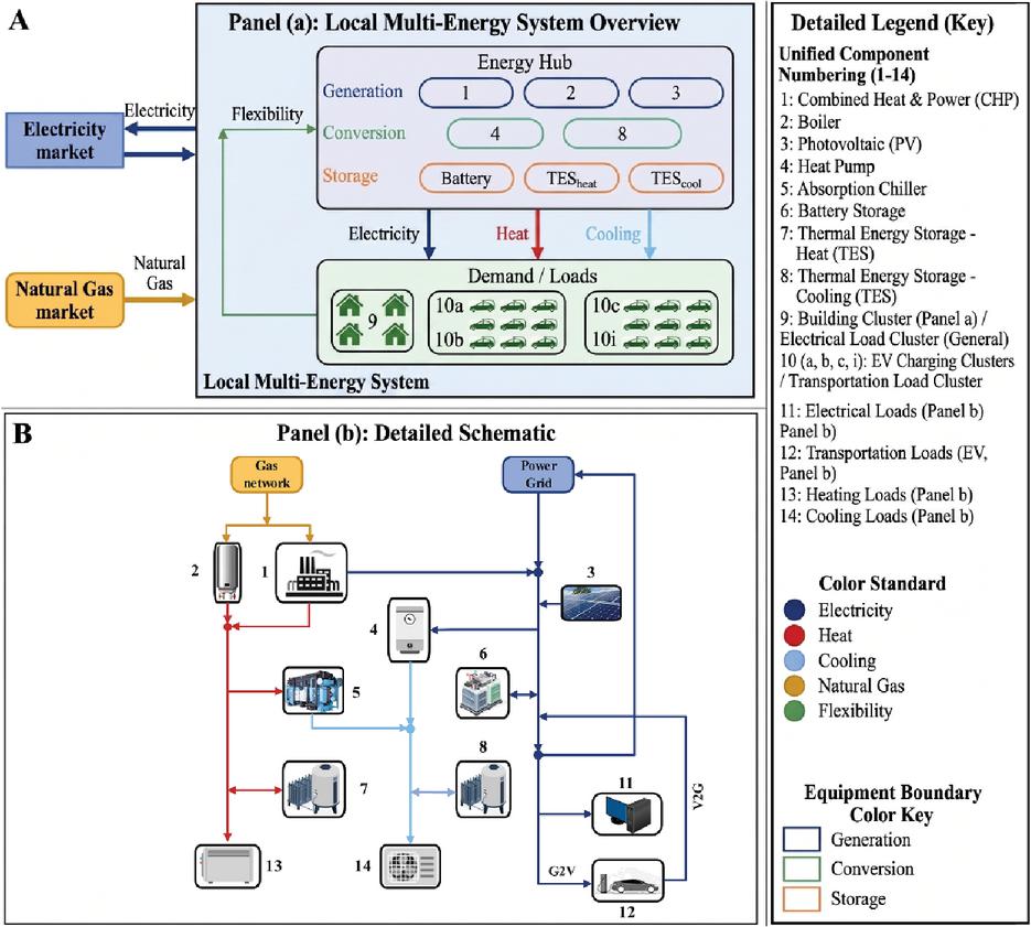
Figure 1 Integrated overview and detailed energy-flow schematic of the local multi-energy system (LMES) for operational optimization.
The entire methodological process of the proposed scheduling framework is illustrated in Figure 2. Firstly, the system configuration of LMES is set and time-dependent data are collected. Then, models of the system elements and the flexibility of PEV are developed. Besides, operational constraints, energy-balance equations, and objective functions are defined. Next, the weighted-sum optimization problem is solved repeatedly for various values of the weighting factor. The solutions obtained are then utilized to plot the Pareto frontier and carry out the subsequent operational analysis.
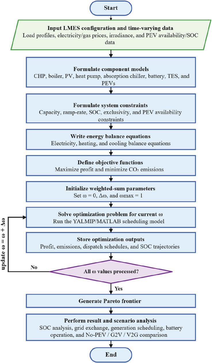
Figure 2 Algorithmic flowchart of the proposed multi-objective LMES scheduling framework.
2.2 System Modeling
The following sections describe how energy technologies and systems are formulated and analyzed within the LMES framework.
2.2.1 Modeling of the CHP unit
Both thermal energy and electricity are produced concurrently by the CHP system. This system’s electrical power output at time t can be written below [29]:
| (1) | |
| (2) |
Here denotes the natural-gas flow rate supplied to the CHP unit, expressed in Nm3/h, , signifies the lower heat value of NG, and implies the electrical efficiency of the CHP. and signify the CHP power output for self-consumption within LMES and for sale to the wholesale market, accordingly.
The CHP unit’s thermal energy output is determined by
| (3) | |
| (4) |
The CHP system’s thermal power is denoted by , and its thermal efficiency is denoted by . The heat fractions needed to cater to the heating and cooling load via the absorption chiller are and , respectively.
2.2.2 Modeling of the auxiliary boiler
The building cluster’s heating needs are satisfied by the backup boiler in tandem with the CHP system. The following is one way to model it:
Gas Usage by the Boiler:
| (5) |
where denotes the natural-gas flow rate consumed by the auxiliary boiler at time t, expressed in ; is the boiler heat output in kW; is the boiler thermal efficiency; and is the lower heating value of natural gas in .
Distribution of Heat:
| (6) |
where the fraction of heat used to satisfy the heating, demand is denoted by , and the fraction of heat allotted for cooling purposes by .
2.2.3 Modeling of the PV unit
The photovoltaic (PV) system’s power production is stated as follows [30, 31]:
| (7) |
where is the photovoltaic array’s area, and is the PV system’s electrical efficiency. The solar irradiance at time t is denoted by .
Two components comprise the overall PV power output: the energy used within the LMES and the excess power sold to the grid. This relationship can be shown as follows:
| (8) |
The power provided to the LMES for internal usage is denoted by , while is the PV power output for selling in the wholesale market.
2.2.4 Modeling of the heat pump and absorption chiller
Depending on whether heating or cooling needs are being met, the LMES’s heat pump can function in two different modes. When the heat pump is in heating cycle, the power needed to achieve the target heating rate is determined by:
| (9) |
The electrical power used by the heat pump to supply the thermal energy is written as . The heat pump’s COP in the heating cycle is denoted by .
Similar formulas for cooling output are used in the modeling technique when the heat pump is in the cooling cycle.
To satisfy the cooling demand, the absorption chiller transforms thermal energy from the auxiliary boiler and CHP systems into cooling energy. The operation of the absorption chillers can be represented as follows:
| (10) |
signifies the chiller’s cooling energy utilized to meet the cooling load, and implies the COP of the absorption chiller.
2.2.5 Modeling of the storage system
To improve flexibility and facilitate energy balancing, the LMES uses a battery system for electrical energy storage. The battery’s SOC at every given time step t is represented using the following model [32, 33]:
| (11) |
Where the SOC at time t is displayed by . is the previous state of charge, and signify the charging and discharging power at period t, and and signify the charging and discharging efficiencies, respectively. Battery Capacity is the battery’s total capacity.
One way to model thermal energy storage is as follows:
| (12) |
where represents the thermal energy retained at time ; represents the thermal energy retained in the preceding time step; represents the storage efficiency accounting for thermal losses; and and signify the charging and discharging heat rates, accordingly. A similar model can be deployed for cooling thermal energy storage.
2.2.6 Modeling of PEVs
PEVs are grouped into clusters inside the LMES, each of which is distinguished by particular characteristics, including (1) battery size, (2) arrival and departure timings at the charging stations, (3) the initial SOC upon arrival, and (4) the targeted SOC at departure. In the proposed model, the traffic pattern of each PEV cluster is represented by its parking availability window at the charging station, defined by the arrival time and the departure time. This window determines when a vehicle is physically available to participate in charging or discharging, while outside the window the charging and discharging powers are set to zero. Customer preferences are enforced through the initial state of charge at arrival and a minimum required state of charge at departure, ensuring that the optimized schedule satisfies the users’ mobility needs and departure readiness. Both G2V and V2G configurations of operation are possible for PEVs.
Before reaching and after leaving the charging stations, PEVs are simulated as:
| (13) | |
| (14) | |
| (15) |
When t is either earlier than or later than for every .
The PEVs’ operation during the parking period is characterized below:
(i) Initial SOC at Arrival:
| (16) |
(ii) SOC Update for Charging and Discharging While Parking:
| (17) |
(iii) SOC at Departure:
| (18) |
where and are the initial and desired SOC at the arrival and departure times, respectively, and , and represent the PEV’s charging, self-discharge, and market discharging capabilities, respectively. The battery capacity of PEV i in cluster is defined as Battery Capacity. In cluster k, the charging and discharging efficiencies of PEV i are represented by and .
3 Mathematical Formulation of the MOO Model
An MOO problem is developed below, drawing on the LMES modeling discussed in the previous part, to determine the optimal ways to operate the technologies and systems, thereby maximizing the profit of the LMES operator while minimizing the environmental impact.
3.1 Formulation of System Constraints
3.1.1 Operational constraints of the CHP unit
The capacity and ramp rate constraints are the two primary constraints that affect the operation of the CHP unit. These constraints are stated as follows:
Capacity Constraint:
| (19) |
Ramp Rate Constraint:
| (20) |
where denotes the CHP’s electrical power output at time t, and and signify the minimum and maximum power output limits, respectively. The binary variable indicates whether the CHP is operating at time t. The maximum permitted decreases and increases in CHP power during a single time step are represented by RampDown and RampUp.
3.1.2 Operational constraints of the auxiliary boiler, heat pump, and absorption chiller
Capacity constraints, which limit energy production within reasonable limits, are a frequent operational constraint for many energy systems. The auxiliary boiler is subject to the following capacity restriction:
| (21) |
The capacity constraints for the absorption chiller and heat pump is also stated in the same way, guaranteeing that their outputs stay within specified limits.
3.1.3 Operational constraints of the storage system
Besides the operation cycle specified in Equation (11), the battery must cater to the operational requirements below:
Charging Power Constraint:
| (22) |
Discharging Power Constraint:
| (23) |
Exclusive Operation of Charging and Discharging:
| (24) |
State of Charge (SOC) Constraint:
| (25) |
3.1.4 Operational constraints of PEVs
To explicitly link mobility behavior to the optimization model, PEV traffic patterns are captured through arrival and departure times that define the feasible charging and discharging window, while user preferences are captured through minimum state of charge requirements at departure. The following additional operational constraints are added to the PEV operating modes specified in the earlier equations:
Charging Power Constraint:
| (26) |
Discharging Power Constraint:
| (27) |
Mutual Exclusivity of Charging and Discharging:
| (28) |
State of Charge Constraint:
| (29) |
3.1.5 Energy balance constraints of the LMES
To make sure that the supply of thermal, cooling, and electrical energy is appropriately matched with the corresponding demands, the energy balancing restrictions are essential. For power, heating, and cooling, these limitations are stated as follows:
Power Balance:
| (30) |
Heating Balance:
| (31) |
Cooling Balance:
| (32) |
3.2 Formulation of Objective Functions
3.2.1 Economic performance objective function
In this study, the LMES operator is modeled as an energy-service provider and aggregator. The operator supplies electricity, heating, and cooling to the building cluster at retail tariffs, purchases electricity from the wholesale market and natural gas from the gas market, and schedules local generation and storage. Moreover, the operator pools electrical flexibility from distributed generators and V2G-enabled PEVs and can also be a seller of the exported electricity to the wholesale market. Hence, operator profit is the net daily cash flow, which is equal to the total revenues less the total costs of energy procurement and V2G remuneration.
The financial goal is to boost LMES’s profit through:
(1) Revenue from providing end users with thermal and electrical energy.
(2) Revenue from the wholesale market sale of power derived from distributed energy sources.
(3) The revenue generated by exporting electricity from V2G-enabled PEVs to the wholesale market.
(4) Profits from PEV owners’ purchases of electricity for charging.
(5) The cost of buying natural gas and electricity to run the system.
(6) Costs associated with purchasing electricity from PEV owners for V2G operations.
It is formulated as:
| Profit | ||
| (33) |
Here, the flexibility of PEVs is considered as the amount of electric energy that can be released from V2G-enabled PEVs back to the wholesale market. In case the PEV discharging is consumed internally within the LMES, it does not lead to wholesale revenue; rather, it decreases the imports from the grid and is therefore shown as a lower cost of energy procurement. Where:
| (34) | ||
| (35) | ||
| (36) |
This exported-energy term is denoted by in the revenue formulation.
| (37) | ||
| (38) | ||
| (39) |
where Profit is the total profit from revenue minus energy costs; is revenue from selling electricity, heating, and cooling to end-users; is revenue from selling flexible DG electricity in the wholesale market; is revenue from PEVs selling electricity back to the grid; is revenue from PEV owners purchasing electricity; Cost is the total cost of purchasing energy; Cost is the cost of electricity transactions with PEV owners in V2G mode; and are prices of electricity, heating, and cooling sold to end-users at time , respectively; and is the electricity price in the wholesale market at time . The pricing assumptions adopted in this study are as follows: the retail electricity tariff applied to PEV charging, , is set equal to the electricity selling price to end-users, . For V2G operation, the operator remunerates PEV owners at , where captures the aggregation margin and transaction costs.
3.2.2 Environmental performance objective function
With emissions assessed over time, the environmental objective function reduces emissions from fossil fuel-based energy systems, taking into account both natural gas and grid electricity consumption. This can be expressed numerically as:
| (40) |
where represents the carbon intensity of natural gas, and refers to the carbon intensity associated with the electricity purchased from the grid. These values indicate the amount of emitted per unit of energy produced, with the grid’s emissions depending on the fuel composition used for power generation [34].
3.3 Multi-Objective Optimization Approach
Using a weighted sum approach, the optimization issue strikes a balance between maximizing operator profit and reducing emissions, thereby satisfying both economic and environmental goals concurrently. The expression for the combined objective function is:
| (41) |
Where is the weight assigned to the economic objective and is a scaling constant used to balance the numerical magnitudes of the two objectives. To construct the Pareto frontier, is swept uniformly over with a fixed step of , and the optimization problem is solved for each value, yielding a discrete set of trade-off solutions. The extreme cases and correspond to the economic and environmental single-objective optima, respectively, while intermediate values represent compromise solutions. Since Profit and Env have different units and numerical scales, a fixed scaling constant is used to prevent unit-driven dominance in the weighted-sum objective. In this study, is computed once from the two extreme single-objective solutions and then kept fixed for all values in the Pareto sweep. where Profit, Profit, and are obtained from the solutions at and . The resulting value of is then kept fixed for all values in the Pareto sweep.
4 Result Analysis and Optimization-Based Case Study
A multi-objective optimization model for an LMES serving office buildings in Turin, Italy (climatic zone E), which incorporates CHP units, PV generation, thermal loads, and battery storage, is implemented using the YALMIP toolkit in MATLAB. The terms residential, commercial, and industrial are used to denote PEV user clusters characterized by distinct availability windows and departure SOC requirements. The LMES demand profiles correspond to an aggregated office-building case study, and end-use electricity, heating, and cooling demands are not segmented by customer type; segmentation is applied on the PEV side through enforceable mobility and SOC constraints. Using three PEV categories, the case study simulates a January day with an hourly resolution. The numerical study focuses on a single representative winter weekday in January with an hourly time step. This choice is made for two reasons. First, the adopted input datasets for building electric and heating demand, Turin irradiance used for PV generation, and the hourly electricity and gas market prices are reported for a typical winter day in January, enabling traceable and reproducible benchmarking. Second, the objective of this work is to analyze intra-day operational trade-offs and technology coordination within a day-ahead scheduling horizon; extending the horizon to multiple seasons or an annual time series would introduce additional inter-day storage and behavioral variability that is outside the scope of the present benchmarking exercise. Therefore, the reported results should be interpreted as representative day-level operational insights rather than year-round performance guarantees. In Section 4.1, input parameters are explained. Sections 4.2–4.8 evaluate the Pareto frontier, SOC profiles, grid flows, generation profiles, thermal load, PEV integration, and battery management.
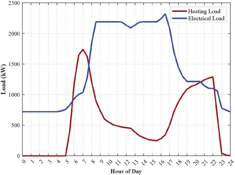
Figure 3 Electrical and Heating Load Profiles of the Building Cluster over a Representative Winter Day in January.
4.1 Model Input Parameters
One hundred small office buildings are intended to be served by the suggested LMES configuration. Based on in-depth surveys of tertiary-sector buildings in cold climate zones, such as zone E in Italy, Figure 3 displays sample hourly profiles of heating and energy use for a typical winter day in January [35]. The demand profiles exhibit notable peaks in the morning and evening, corresponding to heating needs and occupancy patterns. Turin’s meteorological records serve as the basis for the hourly solar irradiance data used to calculate PV generation [36]. Based on historical January 2020 data from the Italian energy markets, Figure 4 displays the constant gas market price (GM) and dynamic electricity market price (EM) used in the economic analysis [37]. The following assumptions apply to the case study. The simulated horizon is 24 hours with hour, representing a typical winter weekday operating condition. Demand and irradiance profiles correspond to winter conditions in Turin, and market prices are taken from hourly January data. Emission factors for grid electricity and natural gas are treated as constant over the horizon. Storage devices operate within their specified SOC limits, and the analysis does not model inter-day carryover effects beyond the 24-hour boundary. PEV participation is constrained by segment-specific availability windows and departure SOC requirements, which represent mobility-driven charging opportunities within the selected day. The most recent technical information about the system’s energy components is shown in Table 1. Gas and electricity are assumed to have carbon intensities of 0.202 and 0.354 kg , respectively [38, 39], by accepted European environmental impact assessment criteria.
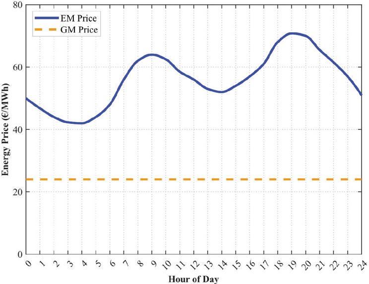
Figure 4 Hourly price profiles of electricity and gas markets.
Table 1 Technical parameters and reference values of system equipment
| Capacity | Efficiency | Charge | Discharge | SOC | |
| Component | [kW or kWh] | [%] | Rate [kW] | Rate [kW] | Range |
| CHP | 100 | 80 | nan | nan | None |
| PV | 200 | 14 | nan | nan | None |
| Battery | 1000 | 90 | 100.0 | 100.0 | 0.2–1.0 |
| PEV | 40 | 95 | 7.2 | 7.2 | 0.4–1.0 |
| Heat Pump | 60 | 300 | nan | nan | None |
4.2 Pareto Frontier Analysis
As shown in Figure 5, the Pareto frontier exhibits the expected trade-off between environmental and economic performance. The environmental optimum corresponds to approximately 1800 kg with an operator profit of about 12000$, whereas the economic optimum reaches approximately 22000$ at about 3500 kg . Intermediate points represent compromise solutions between these two extremes.
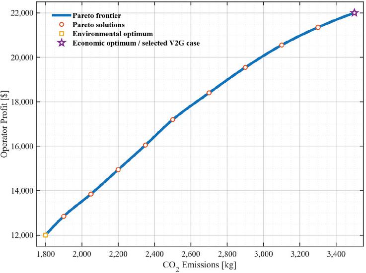
Figure 5 Pareto frontier of the V2G-enabled LMES under multi-objective optimization.
4.3 Clustered SOC Analysis of PEVs
To clarify how the three PEV clusters differ in operational terms, their segment-level operational characteristics over the optimized daily schedule are summarized in Table 2, providing the basis for interpreting the SOC trajectories discussed in this subsection.
Table 2 Segment-level operational characteristics inferred from the optimized daily schedules
| Segment | Residential | Commercial | Industrial |
| Initial SOC | 0.90 | 0.50 | 0.80 |
| Approximate SOC range | 0.90–1.00 | 0.20–0.80 | 0.40–0.80 |
| Peak/minimum SOC timing | Reaches 1.00 at about 3–4 h and remains near full until about 23 h | Peaks near 0.80 at about 7 h; minimum near 0.20 at about 19–20 h | Minimum near 0.40 at about 13–14 h; recovers by 24 h |
| Dominant charging phase | 1–4 h | 1–7 h and 20–24 h | 14–24 h |
| Dominant discharging phase | very limited, mainly near 23–24 h | 7–20 h | 1–14 h |
| Operational interpretation | Intermediate flexibility with a pronounced mid-day depletion and recovery pattern | Highest intra-day SOC swing and strongest time-varying flexibility | High state-of-charge availability with limited intra-day flexibility requirement |
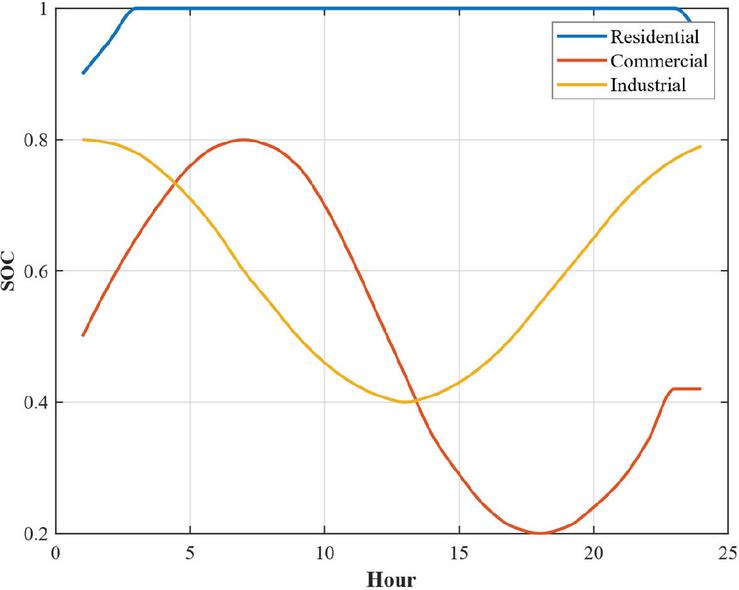
Figure 6 Clustered SOC profiles of PEVs over 24 hours based on user types.
Hourly state-of-charge trajectories for the three PEV clusters (Residential, Commercial, and Industrial) over the 24-hour period are displayed in Figure 6. The Residential cluster always has the highest SOC level: it is about 0.90 at hour 1, it gets to 1.00 at about hours 3–4, and it stays more or less saturated close to 1.00 until hour 23, only slightly dropping to about 0.97–0.98 by hour 24. In contrast, the Commercial cluster exhibits the largest SOC variation, rising from roughly 0.50 at hour 1 to a peak near 0.80 around hour 7, then decreasing steadily to its minimum of approximately 0.20 around hours 19–20, before recovering to about 0.42 by hour 24. The Industrial cluster exhibits an intermediate pattern: SOC falls from 0.80 at hour 1 to a low of about 0.40 at hours 13-14 then it slowly grows and is nearly at 0.79–0.80 by hour 24 again. In fact, Figure 6 very clearly illustrates the differentiated SOC motions across the segments, their approximate SOC ranges directly read from the plotted profiles being 0.90–1.00 (Residential), 0.20–0.80 (Commercial), and 0.40–0.80 (Industrial). Such disparities comply with the segment-specific mobility availability windows and departure SOC requirements stipulated in the PEV model that determine when each cluster can most likely perform charging or discharging during the day.
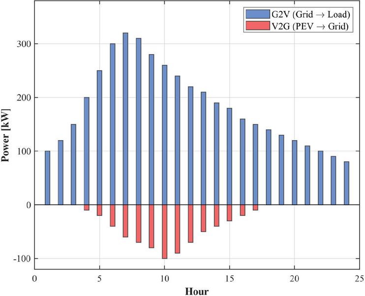
Figure 7 Hourly grid power exchange obtained from the multi-objective optimization.
4.4 Grid Power Flow with Bidirectional PEV Charging
Figure 7 presents the hourly grid power exchange associated with PEV operation, where positive values represent grid-to-vehicle charging (G2V) and negative values represent vehicle-to-grid export (V2G). The G2V profile increases from approximately 100 kW at hour 1 to a morning maximum of about 320 kW around hour 7, after which it gradually declines throughout the day, reaching roughly 180 kW at hour 16 and about 80 kW by hour 24. V2G export appears from about hour 4 (approximately 10 kW), increases in magnitude through the morning, and reaches its strongest export around hour 10 at approximately 100 kW. After the export peak, the magnitude decreases progressively, approaching about 10 kW by hour 17 and becoming negligible thereafter. A notable feature is the concurrent operation of both modes from approximately hours 4 to 17, indicating that charging demand and export support occur within the same day. Quantitatively, V2G partially offsets G2V during this window; for example, at hour 10, G2V is about 260 kW while V2G is about 100 kW, implying a net import of roughly 160 kW and an offset on the order of of the simultaneous G2V magnitude at that hour. Near the G2V peak at hour 7, V2G is approximately 60 kW against roughly 320 kW of G2V, corresponding to a net import of about 260 kW and an offset of about at the peak hour. Importantly, the onset and disappearance of V2G export align with the enforceable availability-window and SOC-at-departure constraints, since charging/discharging actions are set to zero outside the parking intervals in the adopted PEV formulation.
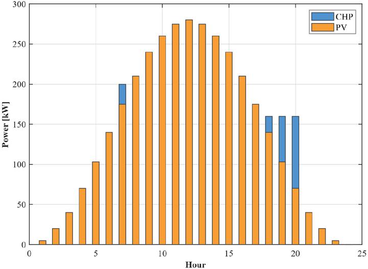
Figure 8 Power generation profiles of CHP and PV.
4.5 Optimized Generation Analysis of CHP and PV Units
Figure 8 compares the hourly electricity generation profiles from photovoltaics (PV) and combined heat and power (CHP). PV output follows a pronounced daytime pattern, rising from near-zero early values to approximately 105 kW at hour 5 and about 140 kW at hour 6, then reaching its maximum of roughly 280 kW around hours 12–13. PV remains above approximately 200 kW over a broad mid-day interval (roughly hours 8–16), before declining to around 175 kW at hour 17, about 105 kW at hour 19, approximately 70 kW at hour 20, and near-zero levels after hour 23. In contrast, CHP appears as a dispatchable contribution concentrated in limited time windows: CHP output is around 200 kW near hour 7, is negligible during the mid-day period when PV is highest, and then reappears in the evening window, reaching approximately 160 kW over hours 18–20. The profiles in Figure 8 therefore indicate distinct timing roles for the two sources, with PV dominating the mid-day generation range (approximately 210–280 kW during hours 8–17) and CHP contributing primarily when PV is lower, particularly around hour 7 and during the evening period.
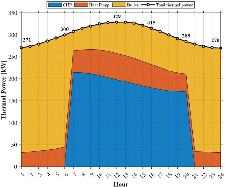
Figure 9 Optimized heat load contribution from distributed thermal resources.
4.6 Thermal Load Breakdown Over Time
Figure 9 depicts the hourly thermal-power shares of the CHP unit, heat pump, and boiler, along with the overall thermal load. The aggregate thermal output starts at around 271 kW in the wee hours, then it ramps up to about 300 kW at hour 6, and it goes on to reach a daily peak of nearly 329 kW around hours 11–12. Subsequently, the total thermal requirement continually decreases, hitting about 315 kW at hour 16, around 285 kW at hour 20, and roughly 270 kW by hour 24. During the night and early morning, the main heating source is the boiler while the heat pump only provides a small supporting contribution and the CHP unit is out of use. For instance, at hour 1, the boiler delivers about 238–240 kW out of around 271 kW total, while the heat pump accounts for about 32–33 kW. A major operational switch is clearly visible from hour 7 and the CHP unit becomes the dominant contributor. At about hour 7, CHP provides nearly 215 kW of a total close to 308 kW, while the heat pump contributes about 48–50 kW and the boiler supplies the remaining 40–45 kW. Around the peak period, the load is more evenly shared: at approximately hour 12, the total thermal power reaches about 329 kW, of which CHP contributes around 195–200 kW, the heat pump about 65–70 kW, and the boiler about 60–70 kW. From the late afternoon onward, the CHP contribution declines steadily, and by hour 20 it falls to roughly 170 kW, while the boiler and heat pump provide about 70–75 kW and 40 kW, respectively. After hour 20, CHP output drops to zero and the boiler again becomes the principal thermal supplier, with the heat pump maintaining a modest auxiliary role. Based on the plotted profiles, the LMES supplies approximately 7.2 MWh of thermal energy over the day, with the boiler contributing about 3.4 MWh, the CHP about 2.7 MWh, and the heat pump about 1.1 MWh, corresponding to approximate shares of 47%, 37% and 16%, respectively.
4.7 Operational Dynamics of the Battery System
Figure 10(a) shows the hourly battery charge and discharge power schedule. Charging occurs primarily from approximately hours 4 to 13, beginning near 20 kW at hour 4, increasing to a maximum of about 90 kW around hour 8, and then declining gradually toward roughly 20 kW by hour 13. Discharging starts around hour 11 (approximately 10 kW), increases in magnitude to a peak discharge of s about 80 kW around hour 16 and then decreases in magnitude toward approximately 10 kW by around hour 21. Figure 10(b) shows the corresponding SOC evolution, rising from approximately 0.50 in the early hours to about 0.76 by hour 8 and around 0.90 by hour 10, reaching its maximum near 0.95 around hours 11–12. After the SOC peak, the curve declines steadily to about 0.84 at hour 14, around 0.67 at hour 16, and approximately 0.55 at hour 18, returning close to 0.50 from hour 20 onward. Across the full day, SOC varies over a range of approximately 0.50 to 0.95 (). From the hourly power bars, the total charged energy is approximately 0.56 MWh and the total discharged energy is approximately 0.52 MWh, indicating that the battery shifts on the order of 0.5–0.6 MWh across the day under the plotted schedule.
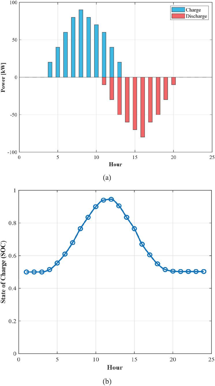
Figure 10 Battery operation profiles obtained from the optimization model: (a) hourly charge/discharge power profile of the battery system. (b) SOC variation over 24 hours.
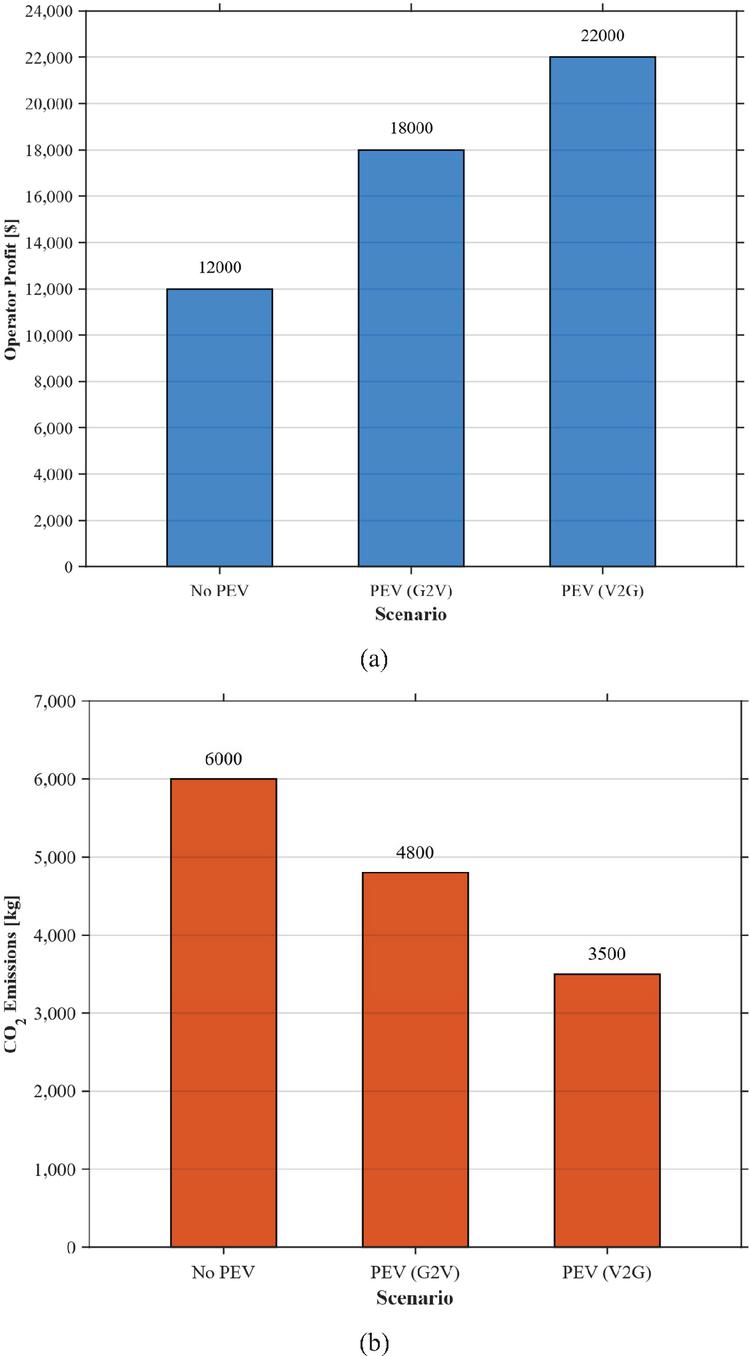
Figure 11 Optimization-based comparison of economic and environmental performance.
Table 3 Operator’s economic profit in different PEV operational scenarios
| Scenario | Operator Profit [$] |
| No PEV | 12000 |
| PEV G2V | 18000 |
| PEV V2G | 22000 |
Table 4 Comparison of emissions across various PEV operational scenarios
| Scenario | Emissions [kg] |
| No PEV | 6000 |
| PEV G2V | 4800 |
| PEV V2G | 3500 |
Table 5 Scenario-based analysis of economic and environmental indicators
| Scenario | PEV Present | V2G Active | Profit [$] | Emissions [kg] |
| No PEV | No | No | 12000 | 6000 |
| PEV G2V | Yes | No | 18000 | 4800 |
| PEV V2G | Yes | Yes | 22000 | 3500 |
Table 6 Impact of PEV integration on system economic and environmental performance
| Scenario | PEV Present | Profit [$] | Emissions [kg] |
| No PEV | No | 12000 | 6000 |
| With PEV(G2V) | Yes | 18000 | 4800 |
| With PEV(V2G) | Yes | 22000 | 3500 |
Table 7 Impact of V2G activation on system economic and environmental performance
| Scenario | V2G Active | Profit [$] | Emissions [kg] |
| With PEV(G2V) | No | 18000 | 4800 |
| With PEV(V2G) | Yes | 22000 | 3500 |
4.8 Scenario Comparison of PEV Impacts
Figures 11(a) and 11(b) compare the three operational scenarios, namely No PEV, PEV (G2V), and PEV (V2G), in terms of operator profit and total CO emissions, with the corresponding numerical values summarized in Tables 3–7. As shown in Figure 11(a), the lowest operator profit is obtained in the No PEV case, at approximately 12000$. When PEVs are introduced in G2V mode, the operator profit increases to about 18000$, indicating that even unidirectional charging can improve the economic performance of the LMES. The highest profit is achieved in the V2G scenario, where operator profit reaches approximately 22000$. Relative to the No PEV case, this corresponds to an increase of about 83%, while the V2G case also improves profit by about 22% compared with the G2V scenario. Clearly the results in Figure 11(b) have a pattern that Environmental performance is one of the main features of the trend observed. emissions caused by No PEV case are the highest and are almost 6000 kg. emissions through G2V operation is still at a level of the 4800 kg, which is almost 20% less than the baseline case. Emissions as low as these can go as a result of V2G scenario as recorded the lowest which in time of the total emissions of can be lowered to 3500 kg. This is a reduction of about 42% in No PEV case and about 27% in G2V case, overall. In general, the comparison of scenarios depicts a No PEV to G2V improvement and also G2V to V2G improvement. V2G is the best in the combined effect in the present scenarios by the way of providing the highest operator profit with the lowest CO emissions as well, which indicates the economic and environmental benefits of bidirectional PEV integration in the LMES.
5 Conclusions
To manage Local Multi-Energy Systems (LMES) with Plug-in Electric Vehicles (PEVs) while striking a balance between environmental sustainability and economic viability, this study presents an MOO framework. Using photovoltaics, combined heat and power (CHP) units, thermal storage, and PEVs with vehicle-to-grid (V2G) and grid-to-vehicle (G2V) capabilities, the model combines gas carriers, electricity, heat, and cooling. By considering time-varying operational profiles, such as shifting electricity prices and variable renewable generation, it maximizes operator profit while reducing emissions. The Pareto frontier analysis reveals a clear trade-off between environmental and economic objectives, with the sampled solutions spanning approximately 1800–3500 kg and 12000$–22000$. Compared with the No-PEV case, the G2V scenario increases operator profit from about 12000$ to about 18000$ while reducing emissions from about 6000 kg to about 4,800 kg. When V2G is enabled, operator profit rises further to about 22000$ and emissions decline to about 3500 kg, indicating that bidirectional PEV participation provides the most favorable combined outcome among the examined scenarios. By utilizing PEVs as distributed energy resources to reduce peak demand, V2G enhances grid flexibility. The framework’s innovation lies in its comprehensive integration of multi-carrier systems, which fills in the gaps left by earlier research that concentrated on a single goal. It captures a variety of mobility patterns by grouping PEVs into residential, commercial, and industrial groups, allowing for customized charging strategies. While commercial and industrial fleets offer dynamic flexibility, improving grid responsiveness, residential PEVs offer steady storage during periods of high demand. Energy allocation is optimized through the coordinated dispatch of boilers, heat pumps, and CHP, with heat pumps taking advantage of favorable conditions for efficiency and CHP controlling periods of high demand. A limitation of the present study is that the numerical analysis is restricted to a single representative winter weekday in January; therefore, the reported results should be interpreted as day-ahead operational insights within the selected seasonal context rather than as year-round performance guarantees. Although the proposed optimization framework performs effectively under the modeled conditions, its scalability should still be examined on larger LMES testbeds. In addition to extended scenario assessments to evaluate various grid situations, future research should investigate adaptive algorithms to manage time-varying renewable generation and dynamic mobility patterns. To enable resilient and sustainable energy systems, this study recommends the adoption of scalable optimization and Vehicle-to-Grid (V2G) technologies, providing operators and policymakers with practical insights that can inform their decisions.
Funding
This work was supported by “Research on Performance Evaluation and Optimization Strategies of Science and Technology Business Incubators in Jilin Province” (JJKH20230524SK).
References
[1] W. Kempton and J. Tomiæ, “Vehicle-to-grid power fundamentals: Calculating capacity and net revenue,” J Power Sources, vol. 144, no. 1, pp. 268–279, Jun. 2005, doi:10.1016/J.JPOWSOUR.2004.12.025.
[2] E. Sortomme and M. A. El-Sharkawi, “Optimal charging strategies for unidirectional vehicle-to-grid,” IEEE Trans Smart Grid, vol. 2, no. 1, pp. 131–138, 2011, doi:10.1109/TSG.2010.2090910.
[3] C. Liu, K. T. Chau, D. Wu, and S. Gao, “Opportunities and challenges of vehicle-to-home, vehicle-to-vehicle, and vehicle-to-grid technologies,” Proceedings of the IEEE, vol. 101, no. 11, pp. 2409–2427, 2013, doi:10.1109/JPROC.2013.2271951.
[4] K. Clement-Nyns, E. Haesen, and J. Driesen, “The impact of Charging plug-in hybrid electric vehicles on a residential distribution grid,” IEEE Transactions on Power Systems, vol. 25, no. 1, pp. 371–380, Feb. 2010, doi:10.1109/TPWRS.2009.2036481.
[5] E. Sortomme and M. A. El-Sharkawi, “Optimal scheduling of vehicle-to-grid energy and ancillary services,” IEEE Trans Smart Grid, vol. 3, no. 1, pp. 351–359, Mar. 2012, doi:10.1109/TSG.2011.2164099.
[6] A. Y. Saber and G. K. Venayagamoorthy, “Plug-in vehicles and renewable energy sources for cost and emission reductions,” IEEE Transactions on Industrial Electronics, vol. 58, no. 4, pp. 1229–1238, Apr. 2011, doi:10.1109/TIE.2010.2047828.
[7] J. Hu, H. Morais, T. Sousa, and M. Lind, “Electric vehicle fleet management in smart grids: A review of services, optimization and control aspects,” Renewable and Sustainable Energy Reviews, vol. 56, pp. 1207–1226, Apr. 2016, doi:10.1016/J.RSER.2015.12.014.
[8] J. A. P. Lopes, F. J. Soares, and P. M. R. Almeida, “Integration of electric vehicles in the electric power system,” Proceedings of the IEEE, vol. 99, no. 1, pp. 168–183, Jan. 2011, doi:10.1109/JPROC.2010.2066250.
[9] Z. Yang, K. Li, and A. Foley, “Computational scheduling methods for integrating plug-in electric vehicles with power systems: A review,” Renewable and Sustainable Energy Reviews, vol. 51, pp. 396–416, Nov. 2015, doi:10.1016/J.RSER.2015.06.007.
[10] S. Zhang, C. Wang, B. Wang, and J. Zhu, “Multi-objective Optimization Charging Strategy for Plug-in Electric Vehicles Based on Dynamic Time-of-use Price”.
[11] W. Li, Z. Lin, K. Cai, H. Zhou, and G. Yan, “Multi-Objective Optimal Charging Control of Plug-In Hybrid Electric Vehicles in Power Distribution Systems,” Energies (Basel), vol. 12, no. 13, pp. 1–19, 2019, Accessed: Jul. 22, 2025. [Online]. Available: https://ideas.repec.org/a/gam/jeners/v12y2019i13p2563-d245392.html.
[12] Z. Xie, K. Chen, Q. Wang, K. Tang, and J. Tian, “Research on Application System of Multi-Objective Optimization in Charging and Discharging Strategy of Electric Vehicle,” Proceedings of 2024 IEEE 6th International Conference on Civil Aviation Safety and Information Technology, ICCASIT 2024, pp. 909–913, 2024, doi:10.1109/ICCASIT62299.2024.10828127.
[13] A. A. Karandinou, F. D. Kanellos, A. A. Karandinou, and F. D. Kanellos, “A Method for the Assessment of Multi-objective Optimal Charging of Plug-in Electric Vehicles at Power System Level,” WSEAS Transactions on Systems and Control, vol. 17, pp. 314–323, 2022, doi:10.37394/23203.2022.17.36.
[14] S. Zeynali, N. Rostami, and M. R. Feyzi, “Multi-objective optimal short-term planning of renewable distributed generations and capacitor banks in power system considering different uncertainties including plug-in electric vehicles,” International Journal of Electrical Power & Energy Systems, vol. 119, p. 105885, Jul. 2020, doi:10.1016/J.IJEPES.2020.105885.
[15] L. Zhang, Z. Ying, Z. Yang, and Y. Guo, “Dynamic Multi-Energy Optimization for Unit Commitment Integrating PEVs and Renewable Energy: A DO3LSO Algorithm,” 2024, doi:10.3390/math12244037.
[16] W. Kong, T. Cai, Y. Fan, F. Jiang, and S. Wan, “Multi-objective optimal charging scheduling strategy for electric vehicles considering traffic flow, power grid, and charging stations,” vol. 12165, pp. 74–80, Mar. 2022, doi:10.1117/12.2627941.
[17] W. Cui, N. Cui, T. Li, Y. Du, and C. Zhang, “Multi-objective hierarchical energy management for connected plug-in hybrid electric vehicle with cyber–physical interaction,” Appl Energy, vol. 360, p. 122816, Apr. 2024, doi:10.1016/J.APENERGY.2024.122816.
[18] M. Cuch, J. Vokøínek, and M. Jakob, “Multi-Objective Electric Vehicle Route and Charging Planning with Contraction Hierarchies,” Proceedings of the International Conference on Automated Planning and Scheduling, vol. 34, pp. 114–122, May 2024, doi:10.1609/ICAPS.V34I1.31467.
[19] V. N. Coelho, “Multi-objective microgrid storage planning problem using plug-in electric vehicles,” Apr. 2016, Accessed: Jul. 22, 2025. [Online]. Available: https://repositorio.ufmg.br/handle/1843/RAOA-BC6J8A.
[20] Y. Wang and X. Jiao, “Multi-objective energy management for PHEV using Pontryagin’s minimum principle and particle swarm optimization online,” Science China Information Sciences, vol. 64, no. 1, pp. 1–3, Jan. 2021, doi:10.1007/S11432-018-9595-3/METRICS.
[21] Y. Zhongan, Y. Kang, and S. Haohui, “Multi-objective Optimization of Electric Vehicle Orderly Charging Based on Variable Preprocessing and MOSO,” Lecture Notes in Electrical Engineering, vol. 1161 LNEE, pp. 374–381, 2024, doi:10.1007/978-981-97-0869-7_41.
[22] D. Ribeiro dos Santos, “Exceptional model mining meets multi-objective optimization: Application to plant growth recipes in controlled environments,” p. 255, Oct. 2021, doi:10.34894/VQ1DJA.
[23] S. Zheng, X. Zhu, L. Xu, Z. Xiang, L. Quan, and B. Yu, “Multi-Objective Optimization Design of a Multi-Permanent-Magnet Motor Considering Magnet Characteristic Variation Effects,” IEEE Transactions on Industrial Electronics, vol. 69, no. 4, pp. 3428–3438, Apr. 2022, doi:10.1109/TIE.2021.3073311.
[24] X. Wang, Y. Fan, C. Yang, Z. Wu, and C. H. T. Lee, “Multi-Objective Optimization Framework of a Radial-Axial Hybrid Excitation Machine for Electric Vehicles,” IEEE Trans Veh Technol, vol. 72, no. 2, pp. 1638–1648, Feb. 2023, doi:10.1109/TVT.2022.3207231.
[25] S. Ehtesham and A. Hanif, “Multi-objective Optimization of Plug-in Hybrid Electric Vehicle (PHEV) Powertrain Families Considering Variable Drive Cycles and User Types over the Vehicle Lifecycle,” Technology (Singap World Sci), 2010.
[26] F. Jiao, Y. Zou, X. Zhang, and R. Zou, “Multi-objective optimal energy management of microgrids including plug-in electric vehicles with the vehicle to grid capability for energy resources scheduling,” Proceedings of the Institution of Mechanical Engineers, Part A: Journal of Power and Energy, vol. 235, no. 3, pp. 563–580, May 2021, doi:10.1177/0957650920942998.
[27] H. Li, C. Zheng, X. Zhang, X. Chen, and X. Chang, “Research on multi-objective optimization coordination of plug-in hybrid electric vehicle and distributed generation,” Proceedings of the 5th IEEE International Conference on Electric Utility Deregulation, Restructuring and Power Technologies, DRPT 2015, pp. 2608–2613, Mar. 2016, doi:10.1109/DRPT.2015.7432688.
[28] W. Wang, M. Wang, J. Guo, Y. Liu, P. Zheng, and Z. Fu, “Multi-Objective Optimization of Less-Rare-Earth Interior Permanent Magnet Synchronous Machines Used for Electric Vehicles,” 2019 22nd International Conference on Electrical Machines and Systems, ICEMS 2019, Aug. 2019, doi:10.1109/ICEMS.2019.8921444.
[29] R. Roberto, R. De Iulio, M. Di Somma, G. Graditi, G. Guidi, and M. Noussan, “A multi-objective optimization analysis to assess the potential economic and environmental benefits of distributed storage in district heating networks: a case study,” International Journal of Sustainable Energy Planning and Management, vol. 20, pp. 5–20, Apr. 2019, doi:10.5278/IJSEPM.2019.20.2.
[30] E. D. Mehleri, H. Sarimveis, N. C. Markatos, and L. G. Papageorgiou, “A mathematical programming approach for optimal design of distributed energy systems at the neighbourhood level,” Energy, vol. 44, no. 1, pp. 96–104, Aug. 2012, doi:10.1016/J.ENERGY.2012.02.009.
[31] C. Weber and N. Shah, “Optimisation based design of a district energy system for an eco-town in the United Kingdom,” Energy, vol. 36, no. 2, pp. 1292–1308, Feb. 2011, doi:10.1016/J.ENERGY.2010.11.014.
[32] G. Liu, Y. Xu, and K. Tomsovic, “Bidding strategy for microgrid in day-ahead market based on hybrid stochastic/robust optimization,” IEEE Trans Smart Grid, vol. 7, no. 1, pp. 227–237, Jan. 2016, doi:10.1109/TSG.2015.2476669.
[33] T. Terlouw, T. AlSkaif, C. Bauer, and W. van Sark, “Optimal energy management in all-electric residential energy systems with heat and electricity storage,” Appl Energy, vol. 254, p. 113580, Nov. 2019, doi:10.1016/J.APENERGY.2019.113580.
[34] H. Ren, W. Zhou, K. Nakagami, W. Gao, and Q. Wu, “Multi-objective optimization for the operation of distributed energy systems considering economic and environmental aspects,” Appl Energy, vol. 87, no. 12, pp. 3642–3651, Dec. 2010, doi:10.1016/J.APENERGY.2010.06.013.
[35] U. Ciarniello, G. Orsini, and F. Santi, “1.2. 2-Indagine sui consumi e sulla diffusione delle apparecchiature nel settore terziario in Italia,” Technical Report RSE A5–053452 (In Italian)(2005), 2005.
[36] R. and A.-C. E. (ASHRAE) American Society of Heating, “International Weather for Energy Calculations (IWEC Weather Files) Users Manual and CD-ROM,” 2001, ASHRAE Atlanta, GA. Accessed: Jul. 22, 2025. [Online]. Available: https://www.mercatoelettrico.org/en/.
[37] “Data available from.” Accessed: Jul. 22, 2025. [Online]. Available: https://www.mercatoelettrico.org/en/.
[38] I. P. on C. C. (IPCC) and I. E. A. (IEA), “Guidelines for National Greenhouse Gas Inventories E CO2 Emissions from Fuel Combustion, Highlights,” International Energy Agency, Paris, 2018. [Online]. Available: https://www.iea.org/data-and-statistics/data-product/greenhouse-gas-emissions-from-energy-highlights.
[39] Educogen, “Educogen, The European Educational Tool on Cogeneration, second ed.,” Educogen, 2001.
Biographies

Yan Hou, born in 1980 and originally from Siping, Jilin, is an associate professor at Jilin Normal University with a doctoral degree. He obtained his Ph.D. from Harbin University of Commerce and his Master’s degree from Tianjin University of Finance and Economics. His main research interests include enterprise development strategy and innovation management, entrepreneurship education, business models, and capital operation.

Shuling Yang, born in 1979 and originally from Siping, Jilin, is an associate professor at Jilin Normal University with a master’s degree. She obtained both her Master’s and Bachelor’s degrees from Jilin Normal University. Her main research interests include business English, cross-border e-commerce, and innovation and entrepreneurship education.
Distributed Generation & Alternative Energy Journal, Vol. 41_4, 931–970
doi: 10.13052/dgaej2156-3306.4144
© 2026 River Publishers