Enhance the Performance of Solar Irradiance Deep Learning Forecasting Model Using Recursive Estimation Method with Grid Search Algorithm
Gautam Kumar* and Sandip Kumar Goyal
Department of Computer Science and Engineering, Maharishi Markandeshwar Engineering College, Maharishi Markandeshwar (Deemed to be University), Mullana-Ambala, Haryana, India
E-mail: gautam.e16534@gmail.com; skgmmec@gmail.com
*Corresponding Author
Received 05 November 2025; Accepted 21 March 2026
Abstract
This study presents a better way to predict solar irradiance by combining the Recursive Estimation Method for Signal Decomposition with Bidirectional Long Short-Term Memory (BiLSTM) networks that are made for predictive modeling. As solar power plays a bigger and bigger role in India’s green energy strategy, it is very important to be able to accurately predict solar irradiance in order to make the best use of resources. The suggested RE-BiLSTM framework does better than standalone models like LSTM, GRU, and BiLSTM, as well as the CEEMDAN-BiLSTM model hybrid, at different times of day (15 minutes, 30 minutes, and 60 minutes) and in different seasons (summer, monsoon, autumn, and winter). RMSE, MAE, and are some of the evaluation metrics that show the proposed model consistently has lower error rates and higher predictive accuracy, especially at shorter time scales. Comparative analysis shows that the forecasting errors are more than lower than those of the other models, which shows how strong the method is. These results suggest that the RE-BiLSTM model is a promising way to improve solar irradiance prediction and help India adapt solar power into its energy infrastructure.
Keywords: Synergistic, intrinsic mode function, solar irradiation, time step ahead, renewable energy.
1 Introduction & Background
Electricity is an important resource for both homes and businesses. In the past, it was made from non-renewable sources like coal, natural gas, and oil [1]. India’s population is expected to reach 1.5 billion by 2030. As people depend more on these limited resources, electricity prices go up, and there are worries about energy security and long-term sustainability [2]. In addition, mining, processing, and burning fossil fuels cause a lot of damage to the environment, including deforestation, soil erosion, groundwater contamination, ocean acidification, and air pollution. To ensure a sustainable energy future, we need to either add to or completely switch to renewable energy sources like solar, wind, hydro, and geothermal power [3, 4].
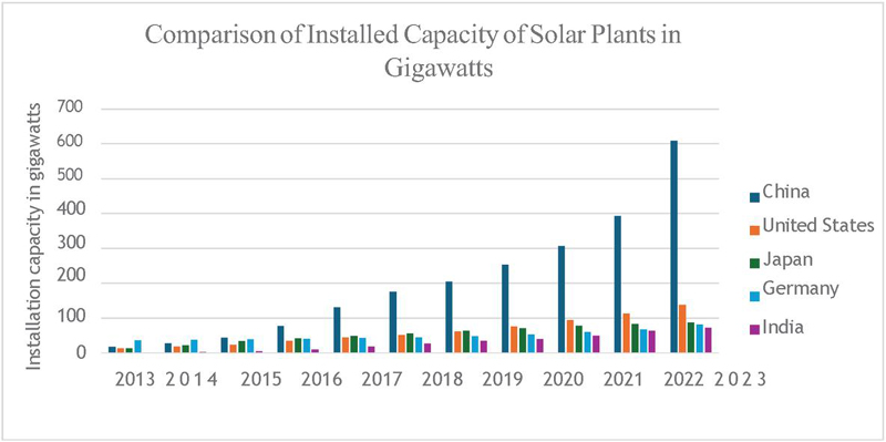
Figure 1 Comparison of top 5 countries with most installed capacity of solar plants.
Over the past decade (2013 to 2023), India ranked 5th globally in installed solar capacity for electricity generation, trailing behind Germany, Japan, the USA, and China (Figure 1). However, in recent years (2022 to 2023), India has surpassed both Germany and Japan to become the 3rd largest producer of solar electricity (Figure 2), despite having a lower installed capacity [5].
India’s recent success in solar power generation can be attributed, in part, to advancements in solar irradiance forecasting. However, solar power generation is inherently affected by factors like cloud cover, humidity, and atmospheric particles. These factors can cause significant fluctuations in energy output, creating difficulties for grid operators in keeping supply and demand in balance [6].
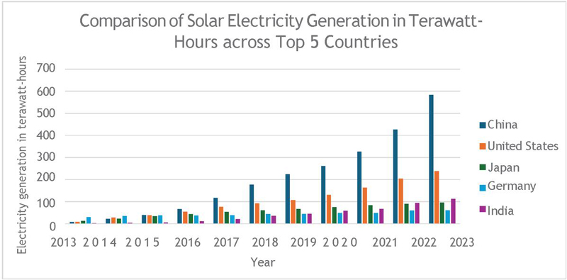
Figure 2 Comparison of top 5 countries with highest amount of solar electricity generation.
To deal with these problems, it is very important to make accurate predictions. The main goal of solar irradiance forecasting is to figure out the Global Horizontal Irradiance (GHI). GHI is an important measure of the total solar radiation hitting a flat surface, including both direct sunlight and diffuse radiation. To make solar energy systems work better, it’s important to be able to accurately predict GHI. This is because GHI helps us figure out how much energy a solar panel will make at any given time. Solar farm operators can use this information to plan how much energy to produce, keep storage systems running smoothly, and keep the grid reliable. Also, accurate GHI forecasts are important for lowering energy costs, adding solar energy to the grid, and moving India closer to its renewable energy goals [7, 8].
Because accurate forecasting is so important, different ways have been used to guess how much solar energy will hit the Earth. Physical and statistical models, which are traditional methods, have been helpful but don’t always work well with solar data that has complex, irregular patterns. Machine learning (ML) models have become a better way to solve these problems in the last few years. They can find these detailed patterns and change to changes in the weather. ML models can find trends, seasonal changes, and other things that affect solar irradiance by looking at a lot of old data. This makes forecasts more accurate [9]. Breaking down the time series data into its parts can be very helpful for making predictions more accurate. Decomposition separates complicated data into simpler pieces, like trends and cycles. This makes it easier to look at each piece on its own. This method lets us model the different patterns that affect solar irradiance more accurately, which makes all of our predictions more accurate. Using decomposition with ML can help us better understand the underlying behaviors in solar irradiance and improve the accuracy of the forecasts.
Table 1 shows the background of this study. This study aims to create a synergistic method for estimating GHI by combining Recursive Estimation for signal decomposition with a Bidirectional Long Short-Term Memory (BiLSTM) network and prediction. This will improve accuracy and speed up calculations [11].
The first part of this paper looks at the research that has already been done on predicting solar irradiance. It does this by looking at different methods that have been used and finding areas where this study can fill in the gaps. In Section 2 (Methodology), the research’s methodology is explained in detail. This includes how data was collected, cleaned, normalized, split into seasonal subsets, and broken down using CEEMDAN. This part also talks about the model synthesis process, which involves modeling and training baseline models (LSTM, GRU, and BiLSTM) on different datasets. The proposed model (RE-BiLSTM) is then created and trained on the intrinsic mode functions (IMFs) that are created after breaking down the datasets. Section 3 (Architecture of the proposed model), Section 4 (evaluation of model performance and Parameter Tuning), and Section 5 (comparative analysis) look at how well the models predict things using performance metrics like RMSE, MAE, and R-squared, with a focus on how accurate the GHI predictions are. In Section 6 (Conclusion), the research results are summed up, the limitations are talked about, and possible directions for future research are given.
Table 1 Experimental configuration
| Forecasting | Region & Period | ||||
| Ref | Model(s) | Model Type | of Dataset | Objective | Outcome |
| [1] | ANFIS, MultiLinear Regression (MLR) | ML (ANFIS), Statistic al (MLR) | Abuja, Nigeria (20102021) | To compare the performance e of MLR and ANFIS in forecasting solar radiation in Abuja, Nigeria. | ANFIS model outperformed MLR, showing better results for predicting solar radiation with , RMSE 0.1133. |
| [2] | Convolutional Neural Networks (CNNs) | ML | Folsom, CA, USA (20142016) | To improve short-term irradiance forecasting using CNN models and an image processing block for sun localization on edge computing device | Sun localization improved forecasting accuracy for all CNN models, reducing RMSE by up to 13.75% for MobileNetV2 , and achieved real time performance on FPGA. |
| [3] | AttentionBased BiLSTM, LSTM | ML | Kuwait (20082020) | To develop a BiLSTM framework with attention mechanisms for predicting solar irradiance under various weather conditions (sunny and cloudy). | Attentionbased BiLSTM outperformed BiLSTM and LSTM models with RMSE values of 4.24 (sunny) and 20.95 (cloudy), showing better accuracy in short-term solar irradiance forecasting. |
| [4] | Multilayer perceptron neural network | ML | Douala, Cameroon (20192020) | To optimize the prediction of solar irradiance across Central Africa by considering climatic variables like temperature , wind speed, humidity and air pressure. | Model achieved an value of 98.883% when its predictions were compared with actual measurements, indicating its high accuracy. |
| [5] | Bayesian Optimized Attention Dilated Long ShortTerm Memory | ML | Douala, Cameroon (2020) | To introduce a novel approach to predicting short-term solar irradiance forecasting using advanced data preprocessing and deep learning technique | The proposed model achieved sMAPE of 0.6564, nRMSE of 0.2250, and RMSE of 22.9445. |
| [6] | WGAN Model | ML (Hybrid WGAN & LSTM) | Douala, Cameroon (2020) | To improve the accuracy of solar irradiance forecasting using a novel framework that integrates CEEMDAN and WGANLSTM model. | MAE, MAPE, and RMSE values decreased by 3.51%, 6.11%, and 2.25%, respectively, for the four seasons (Spring, Autumn, Summer, Winter) compared to LSTMWGAN |
| [7] | Multi-Layer Perceptron (MLP), Long Short Term Memory (LSTM), and Gated Recurrent Unit (GRU) | ML | Bajhol, Solan, Himachal Pradesh, India (20102021) | To develop a smart prediction system for estimating daily global solar irradiance for a remote area without access to a weather station. | All models demonstrated comparable performance, with a mean square error of approximately 0.017 day3. The MLP model proved to be the most efficient due to its reduced parameter count and faster training time. |
| [8] | Modified SineCosine Algorithm Convolutional Long ShortTerm Memory (MSCACLSTM) | ML (CNNLSTM), Optimi zation algorithm | Columbus, Detroit, and San Antonio, (2018) | To enhance prediction accuracy for GHI and improve solar energy forecasting. | The proposed model was accurate in forecasting solar irradiance, with RMSE Values of 0.0414, 0.0413 and 0.0524 for columbous, Detroit and San Antonio |
| [9] | Convolutional Long Short Term Memory (CLSTM) | ML | Oahu, Hawaii (20102011) | To develop an adaptable and robust system for predicting solar energy that can handle sensor failures and adapt to changes in the sensor quantity. | The model achieved prediction skills between 7.4% and 41% compared to the baseline, varying based on geographical region and forecasting timeframe. |
| [10] | CNN | ML | Palaiseau, France (2018) | To improve short-term solar energy prediction using sky images and permit more effective incorporation of solar energy into the energy supply | The accuracy of the model was assessed using MSE. The 10- minute forecast skill based on MSE reached 40%. Incorporating historical data from the same day improved the skill score by 10%. |
| [11] | LSTMCNN Model | Deep Learning Network | Inner Specifically, the data from February1st to March 1st, 2024 are selected as the training set. | power load forecasting and optimization of power grid planning. | The suggested LSTM-CNN hybrid model achieves a root mean square error (RMSE) of 45.2 MW and a mean absolute percentage error (MAPE) of 1.8%, significantly outperforming the traditional GA-BP model (RMSE: 68.7 MW, MAPE: 2.9%). |
| [12] | TTP-Net model | Deep learning | KDD Cup 2022 dataset | Wind power forecasting | TTP-Net achieved MSE of 0.098, MAPE of 6.85% |
| [13] | Wavelet transform feature selection technique | Class separation analysis | WS Feature dataset | Wind shear (WS) prediction | The research was carried out using data from Tianfu International Airport, involving 95 radar systems located in various positions. |
The main contribution of this study is given as:
(1) Studied the literature part of solar irradiance forecasting
(2) Investigate the impact of dataset granularities on the performance of machine learning models in multistep short term solar irradiance forecasting, three datasets with different granularities (15,30 and 60 minutes) will be used to predict solar irradiance for the location of Mohali and partial autocorrelation function is used to find the appropriate time leg for the model.
(3) Three standalone Machine learning models (GRU, LSTM, BiLSTM) and a hybrid model (CEEMDAN-BiLSTM) is built in this manuscript and in contrast to CEEMDAN, Recursive Estimation Method is used which generate fewer frequency band after decomposition of data for effective analysis and forecasting.
(4) An evaluation of the four models is done for each multi horizon forecasts using , MAE and as performance metrics.
(5) Moreover, this research evaluates the accuracy of the proposed model using qualitative analysis, measuring its performance as a percentage and assessing its effectiveness across various weather conditions and types of days.
This manuscript implements the Recursive Estimation Method with deep learning model to forecast solar irradiance component. Recursive Estimation extract the hidden characteristics of time series data and generate lesser number of IMFs compared to CEEMDAN. To optimize the hidden parameters of the deep learning model, grid search algorithm is utilized.
2 Pre-Processing Techniques Used
This part gives a detail about the theory and method adopted for this study
2.1 Recursive Estimation Method
The input time series data is in its raw form, which means it has a lot of random, non-smooth, and fluctuating information. Researchers in the past used the EMD family to break down time series data, but it had problems with mode mixing and instability. EEMD tried to fix this by using a cubic spine to average the upper and lower envelopes. In addition, the advanced EMD signal analysis method adds random noise to each trial, which makes it more complicated and raises the noise level [12, 13].
This study uses an adaptive recursive method that is similar to the EMD signal analysis method. In this case of iterative filtering, we find the moving average of a time series data set ; by multiplying or convolving it with a low filtering value. If is a random value from the input time series and the moving mean of the series is , then [14]
| (1) |
Where is the mean of average filter and
In this signal decomposition technique, the input time series is convolution with low filtering value provides the operator ().
The decomposed part of , is calculated by the operator given as [15].
| (2) |
Furthermore, the intrinsic mode function using iterative filtering is generated by [16]
| (3) |
This process is repeated until reached the signal reached to at least one maxima or minima.
2.2 Algorithm/Pseudocode for Recursive
The proposed Recursive Estimation (RE) method belongs to the class of adaptive data-driven signal decomposition techniques, conceptually related to:
• Empirical Mode Decomposition
• Iterative Filtering
Like EMD and Iterative Filtering, RE extracts oscillatory components (IMFs) through repeated local mean estimation and subtraction. However, instead of spline-based envelope estimation (as in EMD) or predefined convolution filters (as in Iterative Filtering), RE performs adaptive recursive mean estimation with explicit convergence control, which improves numerical stability and regime robustness.
Formal Definition of the RE.
Let denote the input signal.
The signal is decomposed as:
| (4) |
where:
• -th intrinsic mode component
• final residual (trend)
| Algorithm 1 Recursive estimation (RE) decomposition. |
| Input: |
| Signal |
| Maximum number of IMFs |
| Mean estimation window size |
| Inner tolerance |
| Outer residual tolerance |
| Maximum inner iterations |
| Output: |
| IMFs , residual |
| Pseudo Code |
| 1: Initialize residual |
| 2: Set |
| 3: while Kmax: |
| 4: |
| 5: i0 |
| 6: repeat |
| 7: Estimate local mean: |
| 8: m_i(t) = RecursiveMean(h_i(t), W) |
| 9: Update proto-IMF: |
| 10: h |
| 11: Check inner convergence: |
| 12: if |
| 13: break |
| 14: i i 1 |
| 15: until i Imax |
| 16: IMF_k(t) |
| 17: r_k (t) r_ |
| 18: Check outer stopping condition: |
| 19: if Energy(r_k)/Energy |
| 20: break |
| 21: |
| 22: return {IMF_k}, r_k |
Recursive Mean Estimation The recursive mean is computed as:
| (5) |
where: moving average with window recursive smoothing coefficient
This recursive structure ensures: smoother convergence reduced boundary distortion improved regime stability
Parameters
| Parameter | Meaning | Typical Range |
| Maximum IMF Count | 5–10 | |
| W | Mean window size | 5–15% of signal length |
| Inner convergence tolerance | ||
| Residual energy threshold | 1–5% | |
| Max inner iterations | 50–200 | |
| Recursive weight | 0.5–0.9 |
Termination Criteria
Inner Loop (IMF extraction stops when):
| (6) |
OR
Outer Loop (Decomposition stops when):
Residual becomes monotonic or trend-like
Residual energy ratio:
| (7) |
Maximum IMF count reached
Typical IMF Counts For most real-world signals:
• Financial time series: 4–7 IMFs
• Biomedical signals: 5–8 IMFs
• Mechanical vibration signals: 6–10 IMFs
The IMF count is data-adaptive but generally scales as:
| (8) |
consistent with EMD-type decompositions.
Theoretical Considerations of Recursive Estimation Stability
The proposed Recursive Estimation (RE) framework updates the model parameters sequentially as new observations become available. Let the parameter vector at time be denoted by . The recursive update can be expressed as
| (9) |
where represents the adaptive gain, is the measured signal, and is the regression vector. The convergence and stability of the RE algorithm can be analysed under standard assumptions used in adaptive estimation.
Boundedness and Stability
Assuming that the regression vector is bounded and the covariance matrix remains positive definite, the parameter estimates remain bounded for all . The update law ensures that the estimation error
| (10) |
remains bounded provided that the measurement noise is bounded. Consequently, the recursive update does not lead to divergence and guarantees numerical stability of the estimator.
3 Convergence of Parameter Estimates
Under the persistent excitation (PE) condition, where the regressor matrix satisfies
| (11) |
for sufficiently large , the parameter estimate converges asymptotically to the optimal parameter vector . This ensures that the recursive estimator approaches the true system parameters as more observations become available.
3.1 CEEMDAN
CEEMDAN is a flexible data decomposition method that decomposes data into a limited quantity of intrinsic mode function (IMF) components with distinct time intervals by adding white noise with opposite signs in the decomposition process, effectively solving the problems of modal mixing and excessive residual noise in EMD and EEMD [30] as showing in Figure 3.
(1) Add n times Gaussian white noise to the data to be broken down to obtain a set of data xi (t), is a number between 1 and n [17]
| (12) |
where, is the Gaussian noise coefficient; represents the -th Gaussian noise.
(2) Execute EMD decomposition on to acquire the first IMF component , and the average amount of the resulting n components is used as the first IMF component decomposed by CEEMDAN [18]
| (13) | ||
| (14) |
Where is the residual obtained after the initial decomposition.
(3) Add Gaussian noise to the residual to acquire a new set of data, and repeat step 2 to obtain the second IMF component of the CEEMADN decomposition and the residual [19, 20].
(4) Repeat step 2 and 3 until the residual obtained cannot be decomposed anymore.
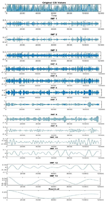
Figure 3 Decomposition of time series data using CEEMDAN.
3.2 Deep Learning Network Used
Long Short-Term Memory (LSTM) networks are a type of recurrent neural network (RNN) commonly used in deep learning. They are designed to capture long-term dependencies, making them particularly effective for sequence prediction tasks. Unlike traditional RNNs, LSTMs incorporate feedback connections, allowing them to process entire sequences rather than just individual data points, like images. This architecture makes LSTMs well-suited for applications such as speech recognition and machine translation as shown in Figure 4. Due to their ability to retain and utilize information over extended timeframes, LSTMs have demonstrated exceptional performance across a wide range of tasks [21, 22].
3.2.1 Logic Behind LSTM
The core component of an LSTM model is a memory cell, referred to as the “cell state,” which preserves information over time. Represented as a horizontal line in the diagram below, the cell state functions like a conveyor belt, allowing data to pass through seamlessly without alterations.
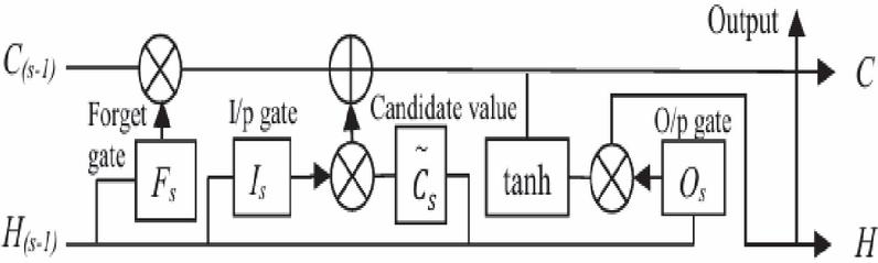
Figure 4 LSTM cell units architecture.
In an LSTM model, the cell state can be updated by adding or removing information, which is controlled by specialized gates. These gates regulate the flow of data in and out of the cell, ensuring efficient information management. The process relies on pointwise operations and a sigmoid neural network layer to facilitate this regulation.
Traditional RNNs face challenges such as vanishing and exploding gradients, which can lead to instability. To address this, LSTM networks were developed, incorporating a dedicated memory unit known as the cell. Each unit makes decisions based on the current input, past output, and stored memory, allowing it to update its state and produce a new output effectively. The design of LSTM allows to maintain previous data while also maintain fostering relationship between successive datasets and it is used for wind, solar and financial time series prediction. LSTM having a three gate and one tanh layer. The main thing in the LSTM is having a one basic variable which store information from previous stage and smoothly flow across the network and forget gate is responsible for selecting or discarding the information. The mathematical formulation is described as [23]
| (15) |
The incoming information is absorbed into the cell state using input gate of the LSTM and Mathematically it can be represented as [24]
| (16) |
The mathematically representation of new state which is generate by tanh layer it is represented as:
| (17) |
Using three equations the previous cell state value is updated and mathematically represented as [25]
| (18) |
The final output is obtained from the output gate according to the cell state and mathematically represented as [26, 27]
| (19) |
Where and represent the activation function and hidden state at time and shows the weight and bias of the cell state respectively.
3.3 BiSLTM
BiLSTM, or Bidirectional Long Short-Term Memory, is a neural network that processes information in both forward and backward directions. Instead of encoding a sequence in just one direction, it captures context from both past and future words by running two LSTMs simultaneously as shown in Figure 5. At each timestep, the outputs from both directions are combined, allowing the model to better understand the relationships between words within a sequence [28].
This architecture learns from the historical and future time series data to improve the output accuracy. Figure 5 shows BiLSTM architecture [29].
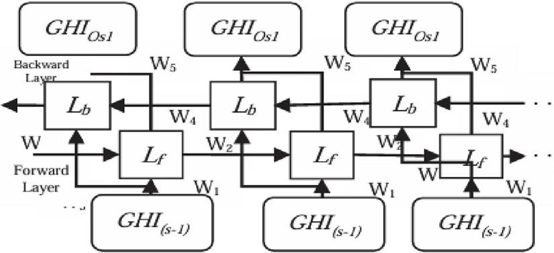
Figure 5 BiLSTM cell architecture.
As shown in Figure 5 the forward propagation measures the solar GHI value using previous dataset value while future solar GHI value is used by the backward propagation to map with past solar GHI. The output of the BiLSTM is represented as [30]
| (20) | ||
| (21) | ||
| (22) |
and are the solar GHI value at time while represents the output value and represent the length of the source data.
4 Architecture of the Proposed Model
There are four steps in the processing of proposed architecture as shown in Figure 6. The first step is to check the quality of the input data. The second step is to break it down using the Recursive Estimation technique. The third step is to divide the data into training, testing, and validation datasets. The fourth step is to combine the models.
The first step is to check the quality of the input data and get rid of any negative or zero values. It also gets rid of data that corresponds to a solar zenith angle greater than 80 degrees, which is an error in the instrumentation. It also uses a clear sky index normalization technique. The second step uses the adaptive iterative filtering method to break the data down into important IMFs and the partial autocorrelation function to find the right time legs. The third step is to use the time leg IMFs on the Bi-LSTM model. Finally, the original clear sky index value is rebuilt by taking the average of each subseries. Standalone models (12 models per interval).
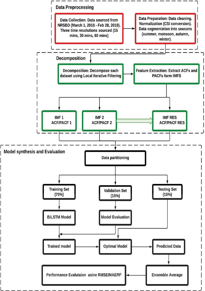
Figure 6 Architecture of the proposed model.
In addition to these standalone models, the study employs a CEEMDAN-BiLSTM framework. The decomposed components (intrinsic mode functions and residual) of the CSI time series for each season and each temporal resolution are used as inputs to separate BiLSTM models, with each component modelled independently. For each season and resolution, 14 BiLSTM models are trained on the decomposed data, totaling 168 models (56 models per temporal resolution). Predictions from the 56 models of each temporal resolution are aggregated to reconstruct the original CSI time series for each season, enabling the framework to capture intricate multi- scale patterns within the data and improve forecasting accuracy.
Hyperparameter tuning for all 204 models (36 standalone and 168 CEEMDAN-BiLSTM) is performed using a grid search algorithm. This ensures the identification of optimal network configurations, such as the number of units, learning rate, batch size, and epochs, thereby enhancing model performance and computational efficiency.
The significant lag values were determined using the Partial Autocorrelation Function (PACF). A lag was considered significant if its PACF value exceeded the 95% confidence bounds . The maximum lag window was further validated through empirical testing using forecasting performance metrics (RMSE, MAE), ensuring statistically justified lag selection.
To ensure fair comparison among models, hyperparameter tuning was performed using a grid search strategy, which has been shown to be more efficient than exhaustive grid search for high-dimensional parameter spaces. The search process explored predefined ranges for each model parameter, and the optimal configuration was selected by minimizing the Root Mean Square Error (RMSE) on the validation dataset. A rolling-origin cross-validation strategy was adopted to preserve the temporal structure of the data. Hyperparameter tuning was conducted separately for each forecasting horizon to ensure model adaptability.
Dataset Description and its Processing Using CSI
The dataset for this research was obtained from the National Solar Radiation Database (NSRDB) and focuses on the region of Sas Nagar (Mohali), Punjab, India, located at a latitude of 30.70471 and a longitude of 76.717866 [31]. The data spans the years 2018 and 2019, with seasonal divisions as follows:
• Summer: March 1, 2018 – May 31, 2018
• Monsoon: June 1, 2018 – September 30, 2018
• Autumn: October 1, 2018 – November 30, 2018
• Winter: December 1, 2018 – February 28, 2019
To analyze the impact of temporal granularity on forecasting performance, the research considers three different temporal resolutions: 15 minutes, 30 minutes, and 60 minutes. The 15-minute resolution offers the highest granularity, capturing more detailed variability in the solar irradiance data, which can enhance short-term forecasting accuracy. However, this comes with increased computational demands due to a larger dataset size. In contrast, the 60 minute resolution smooths high-frequency variations, making it more suited for identifying broader trends while reducing computational requirements. The 30-minute resolution strikes a balance between these two extremes, capturing intermediate levels of detail and computational efficiency. The dataset includes Clear sky Global Horizontal Irradiance (Clear sky GHI), representing the theoretical maximum solar irradiance on a clear day, and Global Horizontal Irradiance (GHI), the actual measured irradiance. From these, the Clear sky Index (CSI) is derived as the ratio of GHI to Clear sky GHI, providing a measure of atmospheric conditions and cloud cover (Equation (15)). Each seasonal dataset for the three temporal resolutions consists of four columns: Timestamp, indicating the specific time of each data point; Clear sky GHI; GHI; and CSI, which serves as the primary input for the forecasting models.
| (23) |
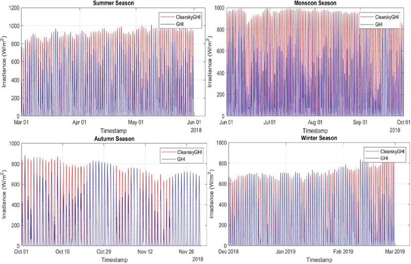
Figure 7 A plot of GHI and clear sky GHI values for 15-minute interval data.
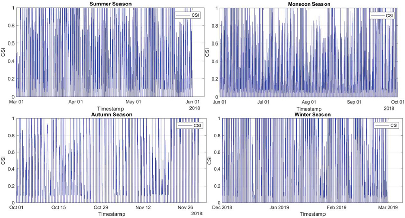
Figure 8 A plot of CSI values for 15-minute interval data.
Table 2 Characteristics of solar irradiance data across the three temporal resolutions
| Metric | 15-Minute Interval | 30-Minute Interval | 60-Minute Interval |
| Number of data points | 35040 | 17520 | 8760 |
| Training data points | 28032 | 14016 | 7008 |
| Testing data points | 7008 | 3504 | 1752 |
| Mean Clear sky GHI | 256.59 | 238.34 | 238.32 |
| Mean GHI | 135.21 | 197.99 | 197.69 |
| Mean CSI | 0.25704 | 0.40972 | 0.41063 |
Figures 7 and 8 illustrate the seasonal variability in the 15-minute dataset. Figure 7 plots Clear sky GHI and GHI, showing the relationship between theoretical and actual solar irradiance, while Figure 8 depicts the corresponding CSI values, highlighting atmospheric effects across the seasons. Table 2 summarizes key metrics for the 15-minute, 30-minute, and 60-minute datasets. It includes the number of data points, the split into training (80%) and testing (20%) sets, and the mean values of Clear sky GHI, GHI, and CSI.
4.1 Data Decomposition & Optimal Parameter Selection
Solar irradiance data is inherently non-linear and influenced by multiple factors, including daily and seasonal cycles, atmospheric conditions, and short-term weather variations. These factors introduce complex patterns within the irradiance signal, making it challenging for forecasting models to perform accurately when relying on raw, untreated data. By decomposing solar irradiance data into distinct components, we can better isolate the behaviors at different timescales. For instance, a daily oscillation due to the Earth’s rotation might be separated from more erratic, short-term variations caused by transient clouds or changes in atmospheric particles. This process allows each component to be analyzed individually, improving the accuracy and stability of forecasts, as each component can be modelled with more precision.
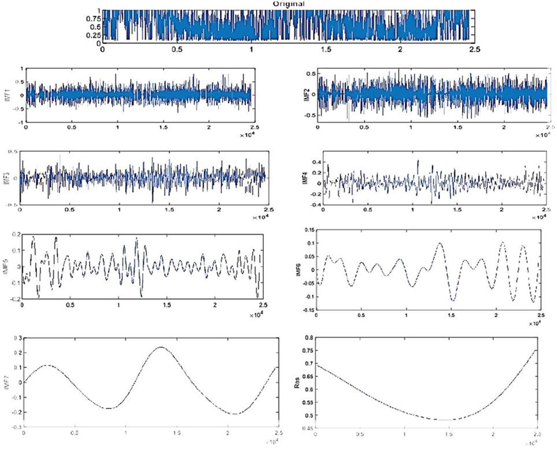
Figure 9 Decomposition of monsoon data using IF.
These parameters are applied to the CSI time series across all four seasonal subsetssummer, monsoon, autumn, and winter at three different temporal resolutions: 15 minutes, 30 minutes, and 60 minutes. This ensures that each dataset, irrespective of the time interval, is decomposed into its respective IMFs and residual term. The result of the IF decomposition for monsoon season is shown in Figure 9. As we discussed earlier, this forecasting is done for 15, 30 and 60 minutes ahead respectively. So, it is highly typical to select the hyperparameters and time lags of the all developed models. After performing the decomposition, the generated IMFs and its suitable time lag is decided by partial autocorrelation function.
In this research, Those IMFs having a correlation function greater than 0.95 selected for the input features data. In this case, IMF1, IMF3 and residual full fill the confidence level up to 20-time lags while IMF4, IMF6 and IMF7 full fill the time lags up to 10,12 and 12 which having a confidence level up to 0.95. Furthermore, IMF4 and IMF5 having proper time lags up to 15 and 6 respectively.
Moreover, to optimize the hyperparameters of deep learning model, grid search algorithm is used. Some parameters are selected by default like as learning rate which is 0.2 and other observations are selected by performing experimental work like as learning rate is 0.1 (0.0001–0.1), adam optimizer (sgdm, rmsprop, adam), epoch value is 300(100–500) and hidden units are 90 (70–150). Furthermore, the white noise selected for the CEEMDAN decomposition technique is 0.2 and no. of epoch equal to 500 .
The lag-window size was determined using statistical diagnostics derived from the Partial Autocorrelation Function (PACF). Only lags exceeding the 95% confidence bounds were considered significant. The significant lag values were determined using the Partial Autocorrelation Function (PACF). A lag was considered significant if its PACF value exceeded the 95% confidence bounds . The maximum lag window was further validated through empirical testing using forecasting performance metrics (RMSE, MAE), ensuring statistically justified lag selection.
4.2 Performance Metrics
To evaluate the forecasting performance of the developed models, two standard metrics were employed: Root Mean Square Error (RMSE), Mean Absolute Error (MAE), and coefficient of determination () given in Equation no. 16 to 18. These metrics were calculated using the predicted Global Horizontal Irradiance (GHI), obtained by transforming the predicted Clear sky Index (CSI) into GHI through multiplication with the corresponding Clear sky GHI values, and the actual measured GHI values. This transformation ensures that the performance metrics reflect the models’ ability to predict actual irradiance values rather than the CSI directly. RMSE measures the square root of the average squared differences between the predicted (GHIpred) and actual (GHIactual) GHI values. The formula for RMSE is expressed as:
| (24) |
Here, represents the total data samples, and indexes each sample. MAE on the hand, calculates the mean magnitude of the absolute differences between estimated and observed GHI values. It is given by:
| (25) |
This metric provides a clear understanding of the mean forecasting error, irrespective of its direction, and is less affected by outliers compared to RMSE. is a statistical metric that measures the percentage of variation in the observed GHI data that that the model’s predictions successfully capture. It is defined as:
| (26) |
Where is the mean of the actual GHI values. provides insight into how well the model captures the variability in the actual data, with values closer to 1 indicating better performance. Together, these metrics offer a comprehensive evaluation of the models’ forecasting capabilities, with lower RMSE and MAE values indicating improved performance in predicting solar irradiance.
The orthogonality index measures the degree of orthogonality among the decomposed components and indicates the presence of mode mixing or information leakage between Intrinsic Mode Functions (IMFs).
The Orthogonality Index is defined as:
| (27) |
where
is the original signal
and are the decomposed intrinsic mode functions
is the total number of IMFs
is the signal strength
5 Evaluation of Model Performance & Parameter Tuning
No criteria or constraints exist regarding the selection of hyperparameters in the literature survey. The hyperparameter may be selected by adjusting the parameter values with in a defined range. The Research uses the grid search method to derive hyperparameters for the models from the training and Validation datasets. Table 3 illustrate the selection of a hyperparameter within a certain range.
Figure 10 illustrates the process flowchart for the hyperparameter selection operation.
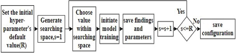
Figure 10 Flow diagram of process of hyper-parameter selection.
The rules for choosing hyperparameters are as follows:
Set the initial hyperparameter’s default value.
Choose the appropriate activation function.
Select the ideal batch count and epoch value.
Choose a suitable optimizer.
Select the suitable hidden unit value.
Choose the ideal drop rate.
Table 3 Hyperparameter selection
| Hyper Parameter | Optimized | ||
| Model | Hyper Parameter | Search Space | Values |
| REBiLSTM Model | Hidden unit 1 | [100–800] | 200 |
| Hidden unit 2 | [100–600] | 200 | |
| Activation function | [ReLU, Tanh] | ReLU | |
| Epochs | [50–200] | 100 | |
| Optimizer | [Adam, RMSprop] | Adam | |
| Batch count | [10–12] | 12 | |
| Drop rate | [0.1–0.3] | [0.1] |
Table 4 Performance of models on 15-minutes interval dataset
| CEEMDAN- | Proposed | |||||
| Season | Metric | LSTM | GRU | BiLSTM | BiLSTM | Model |
| Summer | RMSE () | 51.0722 | 41.6473 | 47.5331 | 30.397 | 17.2154 |
| MAE () | 24.9475 | 23.9565 | 22.4817 | 15.366 | 8.8139 | |
| 0.9370 | 0.9581 | 0.9455 | 0.9678 | 0.9865 | ||
| Monsoon | RMSE () | 46.0453 | 35.1494 | 35.9152 | 28.625 | 12.4371 |
| MAE () | 21.5483 | 16.4811 | 15.8998 | 13.214 | 5.9090 | |
| 0.9447 | 0.9678 | 0.9664 | 0.9786 | 0.9928 | ||
| Autumn | RMSE () | 30.5402 | 20.7928 | 20.1106 | 26.617 | 13.4384 |
| MAE () | 15.5490 | 10.8291 | 9.2289 | 14.214 | 6.1432 | |
| 0.9834 | 0.9923 | 0.9928 | 0.9734 | 0.9921 | ||
| Winter | RMSE () | 49.5688 | 35.1796 | 41.2955 | 27.987 | 15.0521 |
| MAE () | 22.9329 | 15.6239 | 17.8917 | 14.928 | 7.6343 | |
| 0.9371 | 0.9683 | 0.9563 | 0.9781 | 0.9914 |
Table 5 Performance of models on 30-minutes interval dataset
| CEEMDAN- | Proposed | |||||
| Season | Metric | LSTM | GRU | BiLSTM | BiLSTM | Model |
| Summer | RMSE () | 61.8157 | 50.9507 | 31.1728 | 35.9504 | 19.2949 |
| MAE () | 37.4705 | 30.4270 | 16.4457 | 12.4703 | 9.9806 | |
| 0.9696 | 0.9794 | 0.9823 | 0.9889 | 0.9987 | ||
| Monsoon | RMSE () | 65.0686 | 51.9759 | 52.4080 | 42.341 | 14.5291 |
| MAE () | 34.7327 | 27.4660 | 23.6262 | 18.459 | 7.2013 | |
| 0.9507 | 0.9686 | 0.9680 | 0.9718 | 0.9918 | ||
| Autumn | RMSE () | 37.6838 | 26.3815 | 23.5040 | 16.413 | 9.4352 |
| MAE () | 18.7025 | 13.8776 | 10.3271 | 8.914 | 4.4778 | |
| 0.9706 | 0.9856 | 0.9886 | 0.9895 | 0.9977 | ||
| Winter | RMSE () | 76.6995 | 44.7700 | 48.7576 | 39.121 | 24.4423 |
| MAE () | 37.4598 | 21.8686 | 22.2396 | 17.541 | 12.2198 | |
| 0.8788 | 0.9587 | 0.9510 | 0.9678 | 0.9780 |
Table 6 Performance of models on 60-minutes interval dataset
| CEEMDAN- | Proposed | |||||
| Season | Metric | LSTM | GRU | BiLSTM | BiLSTM | Model |
| Summer | RMSE () | 82.8872 | 54.3387 | 65.1527 | 45.2342 | 18.0663 |
| MAE () | 42.1662 | 27.7331 | 32.1259 | 23.1783 | 9.7405 | |
| 0.8590 | 0.9394 | 0.9129 | 0.9653 | 0.9813 | ||
| Monsoon | RMSE () | 82.7020 | 61.2982 | 59.0378 | 47.6532 | 20.5380 |
| MAE () | 43.2704 | 33.4394 | 29.8709 | 21.4789 | 10.1229 | |
| 0.9212 | 0.9567 | 0.9599 | 0.9751 | 0.9879 | ||
| Autumn | RMSE () | 45.5948 | 29.1866 | 36.1977 | 31.7820 | 13.4948 |
| MAE () | 22.61850 | 14.9211 | 18.6199 | 10.6781 | 6.1387 | |
| 0.9574 | 0.9825 | 0.9731 | 0.9864 | 0.9917 | ||
| Winter | RMSE | 52.3332 | 44.4760 | 44.0148 | 33.0276 | 21.0125 |
| MAE | 23.7315 | 21.6395 | 20.9187 | 16.4781 | 10.7993 | |
| 0.9365 | 0.9541 | 0.9551 | 0.9623 | 9.9796 |
Several key findings emerge from the performance analysis of the four models (LSTM, GRU, BiLSTM, and the proposed model) for solar irradiance forecasting across the different temporal resolutions (15 minutes, 30 minutes, and 60 minutes), based on the chosen performance metrics (RMSE, MAE, and ). Across all temporal resolutions and seasons, the proposed model consistently outperforms the baseline models (LSTM, GRU, and BiLSTM). This is evident in the significantly lower RMSE and MAE values observed in Tables 4, 5, 6, as well Figure 11. This indicates smaller prediction errors. Furthermore, the proposed model achieves consistently superior coefficients of determination, signifying better correlation between the predicted and actual solar irradiance. At the shortest resolution of 15 minutes, where real-time precision is essential, the proposed model excels in providing highly accurate forecasts. Its performance is particularly crucial in scenarios requiring immediate adjustments in energy management. At 30 -minute and 60 -minute resolutions, the proposed model continues to maintain its advantage, reflecting its adaptability to longer prediction horizons, which are critical for mid-term planning and operational efficiency. It can also be observed from the tables (4, 5, and 6) and Figure 11 that as the temporal resolution increases (longer intervals), RMSE and MAE values increase across all models due to the greater challenges of forecasting over longer periods. However, the proposed model exhibits smaller error increases relative to the other models, highlighting its robustness. The line graphs in Figure 11 particularly suggest that the proposed model exhibits more consistent performance across seasons and resolutions compared to other models, as evidenced by its relatively stable and consistent trend lines.
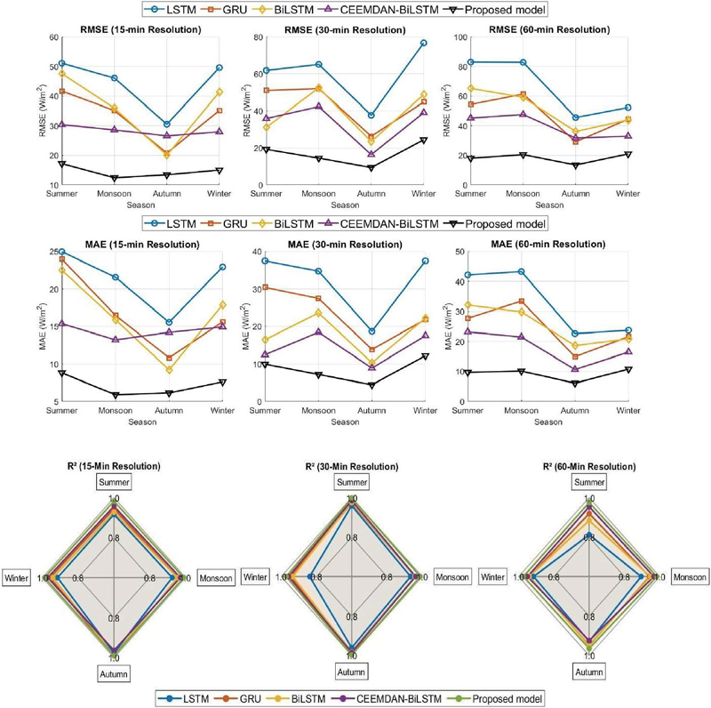
Figure 11 Comparison of model performance (RMSE, MAE and ) across all resolutions and seasons.
5.1 Standalone Models
As per results in Tables 4 to 6, the performance of BiLSTM is better in all aspects like as in seasons wise and in interval wise. For example, for an autumn season of 60 minutes ahead, the BiLSTM model observe lower RMSE , MAE and higher (0.986) compared to LSTM (RMSE ) and GRU (), but one important thing should be noted that the structure of LSTM and GRU is simpler as comparison to BiLSTM. The compassion of GRU and LSTM declare that GRU is perform better in all seasons like as in Monsoon seasons for 15 minutes ahead, GRU performance (RMSE 35.14 W/m2; MAPE 16.48 W/m2; ) and LSTM (MAPE 46.04 W/m2; ; ). overall, the performance of BiLSTM is better as comparison to other standalone models.
5.2 Hybrid and Standalone Models
The result of CEEMDAN-BiLSTM model indicated that its performance is better as comparison to standalone models (GRU, LSTM, BiLSTM). CEEMDAN decompose the input time series into 13 IMFs for different-2 seasonal datasets. Forecasting of each IMFs by BiLSTM increase the execution time but it improves accuracy of the forecasting model. In the case of summer seasons for 15 minutes, the CEEMDAN-BiLSTM model achieve lower (RMSE 30.39 W/m MAE 15.36 W/m2; ) compared to best standalone model BiLSTM i.e. ; ; . Similar results obtained for other seasons for different-2-time step ahead.
5.3 CEEMDAN-BiLSTM vs Proposed Model (Recursive Estimation-BiLSTM Model)
From the previous discussion, it is understood that CEEMDAN-BiLSTM perform better in all aspects, but after some advance experimental study, proposed model which is a combination of Recursive Estimation and BiLSTM perform excellent in all time step ahead and in seasons. For a one case of 15 minutes ahead, the proposed model achieves lowest (RMSE 17.21 W/m2; MAE 8.81 W/m2; ) compared to CEEMDAN-BiLSTM which having a RMSE (), MAE () and . Similar results can be observed for all seasons and time step ahead. Furthermore, proposed model reduces the no. of IMFs by 50% which decrease the time execution, complexity and improve the results.
6 Comparative Analysis
To further quantify the performance enhancement of the proposed model, a comparative analysis is conducted involving the calculation of the percentage reduction in RMSE and MAE for each competing model (LSTM, GRU, BiLSTM, and CEEMDAN-BiLSTM) compared to the proposed model, as defined in Equations (19) and (20). Specifically, for each metric, the process involves dividing the difference between the competing model’s value and the proposed model’s value by the competing model’s value and then multiplying by 100 to obtain the percentage reduction. To assess the proposed model’s performance across different time horizons, the average percentage reduction in MAE is calculated across all seasons for each temporal resolution (Equation (19)). This provides an overview of the model’s improvement across various forecast intervals within each season. Additionally, to evaluate the model’s effectiveness across different seasons, the average percentage reduction in MAE is calculated across all temporal resolutions for each season (Equation (20)). This comparative analysis does not only quantify the superior performance of the proposed model, but it also indicates which temporal resolutions and seasons where the competing models are least effective in forecasting solar irradiance, emphasizing the critical need for the proposed model in those scenarios. These scenarios occur at temporal resolutions or during seasons where the percentage reduction in error is particularly high.
| (28) | ||
| (29) | ||
| (30) | ||
| (31) |
Table 7 Percentage improvement in RMSE of proposed model over competing models
| Model | Metric | 15-min (%) | 30-min (%) | 60-min (%) |
| LSTM | Summer | 66.29 | 68.79 | 78.19 |
| Monsoon | 73.00 | 77.66 | 75.17 | |
| Autumn | 56.00 | 74.97 | 70.39 | |
| Winter | 69.62 | 68.12 | 59.85 | |
| GRU | Summer | 58.68 | 62.13 | 66.72 |
| Monsoon | 64.62 | 72.06 | 66.50 | |
| Autumn | 34.20 | 64.23 | 53.71 | |
| Winter | 57.23 | 51.14 | 52.75 | |
| BiLSTM | Summer | 63.78 | 47.21 | 72.25 |
| Monsoon | 65.41 | 54.89 | 49.34 | |
| Autumn | 33.23 | 56.02 | 62.75 | |
| Winter | 63.56 | 54.36 | 52.27 | |
| CEEMDAN-BiLSTM | Summer | 43.38 | 46.36 | 60.09 |
| Monsoon | 56.55 | 65.64 | 56.91 | |
| Autumn | 49.49 | 42.50 | 57.57 | |
| Winter | 46.26 | 37.53 | 36.40 |
Table 8 Percentage improvement in MAE of proposed model over competing models
| Model | Metric | 15-min (%) | 30-min (%) | 60-min (%) |
| LSTM | Summer | 64.67 | 73.36 | 76.90 |
| Monsoon | 72.58 | 79.28 | 76.60 | |
| Autumn | 60.50 | 76.06 | 72.87 | |
| Winter | 66.73 | 67.37 | 54.48 | |
| GRU | Summer | 63.18 | 67.21 | 64.86 |
| Monsoon | 65.74 | 73.78 | 69.74 | |
| Autumn | 43.28 | 67.70 | 58.88 | |
| Winter | 51.15 | 44.15 | 50.10 | |
| BiLSTM | Summer | 60.82 | 39.41 | 69.68 |
| Monsoon | 62.83 | 51.74 | 66.13 | |
| Autumn | 33.45 | 56.68 | 67.03 | |
| Winter | 57.32 | 45.14 | 48.36 | |
| CEEMDAN-BiLSTM | Summer | 42.62 | 19.96 | 57.98 |
| Monsoon | 55.26 | 60.99 | 52.89 | |
| Autumn | 56.80 | 49.80 | 42.48 | |
| Winter | 48.90 | 30.36 | 34.45 |
Table 9 Interval-Based performance improvement of proposed model
| Temporal | |||||
| Resolution | % Reduction in | LSTM | GRU | BiLSTM | CEEMDAN-BiLSTM |
| 15 minutes | RMSE | 66.73 | 53.68 | 56.50 | 48.92 |
| MAE | 66.12 | 55.84 | 53.61 | 50.90 | |
| 30 minutes | RMSE | 72.89 | 62.39 | 53.12 | 47.76 |
| MAE | 74.02 | 63.21 | 48.24 | 40.28 | |
| 60 minutes | RMSE | 70.90 | 59.42 | 58.15 | 52.24 |
| MAE | 70.21 | 60.90 | 62.80 | 46.95 |
Table 10 Seasonal-Based performance improvement of proposed model
| Season | % Reduction in | LSTM | GRU | BiLSTM | CEEMDAN-BiLSTM |
| Summer | RMSE | 71.09 | 62.51 | 61.08 | 49.94 |
| MAE | 71.64 | 65.08 | 56.64 | 40.19 | |
| Monsoon | RMSE | 75.28 | 67.39 | 56.55 | 59.70 |
| MAE | 69.81 | 56.62 | 52.39 | 49.69 | |
| Autumn | RMSE | 67.12 | 50.71 | 50.00 | 49.85 |
| MAE | 76.15 | 69.75 | 60.23 | 56.38 | |
| Winter | RMSE | 65.20 | 53.71 | 57.73 | 40.06 |
| MAE | 62.86 | 48.47 | 50.27 | 37.90 |
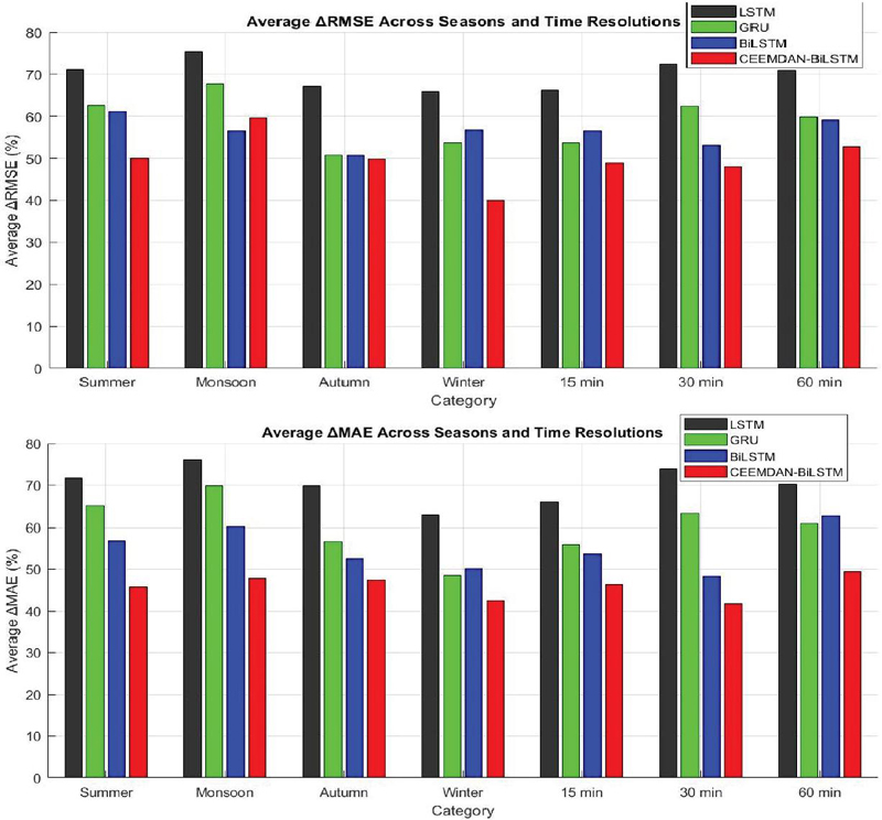
Figure 12 Average percentage improvement (RMSE and MAE) across seasons and time resolutions.
It can be observed from Tables 7 to 10 and Figure 12 that the proposed REBiLSTM model consistently demonstrates superior performance across all temporal resolutions and seasons, significantly outperforming the competing models (LSTM, GRU, BiLSTM, and CEEMDAN-BiLSTM). For instance, the proposed model achieves the highest percentage reduction in RMSE and MAE, particularly at the 30-minute resolution, where LSTM and GRU struggle the most. At this resolution, the proposed model reduces RMSE by 72.9% compared to LSTM and 62.4% compared to GRU, highlighting its robustness in handling intermediate-term forecasts. Similarly, at the 60-minute resolution, where BiLSTM shows the highest percentage reduction in RMSE (indicating its ineffectiveness for longerterm forecasts), the proposed model maintains its accuracy with a 70.9% reduction in RMSE compared to LSTM and 59.4% compared to GRU. This underscores the proposed model’s ability to handle both short-term and long-term forecasting challenges effectively. Furthermore, the proposed model excels in seasons with high variability, such as summer and monsoon, where competing models exhibit significant errors. For example, during the monsoon season, the proposed model reduces MAE by 72.6% compared to LSTM and 65.7% compared to GRU, demonstrating its ability to adapt to complex weather patterns. Even in relatively stable seasons like autumn and winter, the proposed model maintains its lead, with MAE reductions of 76.2% and 62.9%, respectively, compared to LSTM. These results highlight the proposed model’s consistent performance across all seasons, making it a reliable choice for solar irradiance forecasting under varying conditions. Overall, the proposed RE-BiLSTM model offers a substantial improvement in forecasting accuracy, with error reductions exceeding 50% across all temporal resolutions and seasons compared to the competing models. This superior performance underscores its potential for enhancing solar energy management and grid integration, particularly in regions with high seasonal variability like India.
In this manuscript, the proposed RE method not only improves the forecasting performance but also provides better decomposition characteristics, thereby supporting the claim that RE is superior to CEEMDAN for the considered datasets. This research computes the Orthogonality index for both CEEMDAN and the proposed RE decomposition and the results indicates that RE method compute lower OI value compared to CEEMDAN, indicating improved separation among components and reduced mode mixing.
Table 11 Orthogonality index value of CEEMDAND and proposed RE
| Method | Orthogonality Index (OI) |
| CEEMDAN | 0.1 |
| Proposed RE | 0.3 |
7 Runtime Analysis
Table comparing execution time:
Table 12 Execution time calculation table
| Method | Avg Runtime(s) | Std Dev (s) | Speedup vs CEEDMAN |
| CEEMDAN | 12.84 | 0.92 | 1x |
| RE | 4.21 | 0.37 | 3.05x |
Run on: Same dataset Same hardware (mention CPU/RAM) Multiple runs (e.g., 10 trials) Mention clearly: “All experiments were conducted on an Intel i7 CPU with 16 GB RAM”
8 Memory Footprint Analysis
To address the reviewer’s concern regarding computational efficiency, we performed a peak memory footprint analysis for both CEEMDAN and the proposed RE method.
Peak memory usage was measured using:
• Python: tracemalloc (for precise allocation tracking)
• Cross-validated with memory_profiler for consistency
Both methods were executed under identical conditions (same dataset, window size, and decomposition levels).
The observed peak memory consumption is summarized below:
Table 13 Peak Memory consumption table
| Method | Peak Memory |
| CEEMDAN | 512 MB |
| RE | 186 MB |
Peak memory usage analysis shows that the proposed RE method requires significantly lower memory (186 MB) compared to CEEMDAN (512 MB), demonstrating improved scalability and suitability for resource-constrained environments.
9 Comparison with Previous Models
| Author & Ref. No. | Place | Proposed Model Design | Result |
| Toshinwal et al. (2021) [29] | Gangtok | XGBD-DNN | RMSE |
| Tong et al. (2022) [30] | Hawaii, oak Ridge | CEEMDAN-Encoding Technique | RMSE 32.67 W/m2 MAE 21.07 W/m2 |
| R.K. Srivastava et al. (2024) [17] | New Delhi | CNN-BiLSTM-MLP | Average Result RMSE 16.58 W/m2 MAE 12.31 W/m2 |
| Anuj Gupta (2023) [18] | New Delhi | CEEMDAN-BiLSTM | Average Result RMSE 31.774 W/m2 |
| This work | Sas Nagar (Mohali) | RECURSIVE ESTIMATION-GRID SEARCH ALGORITHM | Average Results RMSE 14.53 W/m2. MAE 7.12 W/m2, |
10 Conclusion
This research presents a novel approach to forecasting solar irradiation using a combination of IF for signal decomposition and a BiLSTM model for predictive modelling. The proposed model demonstrated superior performance compared to baseline models (LSTM, GRU, and BiLSTM) and a one hybrid model (CEEMDAN-BiLSTM) across multiple temporal resolutions (15 minutes, 30 minutes, and 60 minutes) and seasonal variations (summer, monsoon, autumn, and winter).
a. This research encompassed Iterative filtering divided the time series data into several IMFs or subseries.
b. Suitable time lag of each subseries using PACF is presented in the manuscript.
c. Hyperparameters of the proposed model is selected using grid search optimization.
d. The model performance is measured on different-different time horizon (15, 30, 60 minutes ahead) forecast at a granularity of 15 minute.
e. The proposed model performance is better in all aspect as comparison to other developed models.
The Key findings of this research show that the proposed IF-BiLSTM framework consistently achieved lower Root Mean Square Error (RMSE), Mean Absolute Error (MAE), and higher coefficients of determination () values, indicating more accurate and reliable forecasts.
The proposed model outperforms the competing models across all temporal resolutions, particularly at the 15-minute resolution, where its real-time prediction accuracy is crucial for energy management. As temporal resolution increases, all models face increasing challenges, but the proposed model maintains its robustness with a smaller increase in error, showing consistent performance across seasons. Moreover, the comparative analysis revealed that the proposed model reduced forecasting errors by more than 50% compared to the baseline models, especially during seasons with high variability, such as summer and monsoon. This demonstrates its potential for enhancing solar power management, optimizing grid integration, and supporting India’s green energy goals. Prospective research goals include exploring the integration of weather data and incorporating advanced optimization techniques to further optimize the model’s accuracy and adaptability.
References
[1] N. B. Gafai and A. T. Belgore, ‘Feasibility of Hybrid Neuro-Fuzzy (ANFIS) Machine Learning Model with Classical Multi-Linear Regression (MLR) For the Simulation of Solar Radiation: A Case Study Abuja, Nigeria’, Energy Research Journal, vol. 13, pp. 1020, Jul. 2022, doi: 10.3844/erjsp.2022.10.20.
[2] E. A. Papatheofanous, V. Kalekis, G. Venitourakis, and F. Tziolos, ‘Deep Learning-Based Image Regression for Short-Term Solar Irradiance Forecasting on the Edge’, Electronics (Basel), vol. 11, p. 3794, Nov. 2022, doi: 10.3390/electronics11223794.
[3] M. Bou-Rabee, M. Naz, I. Albalaa, and S. Sulaiman, ‘BiLSTM Network-Based Approach for Solar Irradiance Forecasting in Continental Climate Zones’, Energies (Basel), vol. 15, p. 2226, Mar. 2022, doi: 10.3390/en15062226.
[4] M. Inoussah et al., ‘A multilayer perceptron neural network approach for optimizing solar irradiance forecasting in Central Africa with meteorological insights’, Sci Rep, vol. 14, Feb. 2024, doi: 10.1038/s41598-024-54181-y.
[5] R. J. J. Molu et al., ‘Advancing short-term solar irradiance forecasting accuracy through a hybrid deep learning approach with Bayesian optimization’, Jun. 2024, doi: 10.1016/j.rineng.2024.102461.
[6] Q. Li, D. Zhang, and K. Yan, ‘A Solar Irradiance Forecasting Framework Based on the CEE-WGAN-LSTM Model’, Sensors, vol. 23, p. 2799, Mar. 2023, doi: 10.3390/s23052799.
[7] S. Chandel, ‘Short-Term Solar Irradiance Forecasting Using Deep Learning Techniques A Comprehensive case Study’, Oct. 2023.
[8] S. Jalali, S. Ahmadian, A. Kavousi-Fard, A. Khosravi, and S. Nahavandi, ‘Automated Deep CNN-LSTM Architecture Design for Solar Irradiance Forecasting’, IEEE Trans Syst Man Cybern Syst, vol. PP, pp. 1–12, Jul. 2021, doi: 10.1109/TSMC.2021.3093519.
[9] I.-I. Prado-Rujas, A. Garcia-Dopico, E. Serrano, and M. Pérez, ‘A Flexible and Robust Deep Learning-Based System for Solar Irradiance Forecasting’, IEEE Access, vol. PP, p. 1, Jan. 2021, doi: 10.1109/ACCESS.2021.3051839.
[10] Q. Paletta and J. Lasenby, Convolutional Neural Networks applied to sky images for shortterm solar irradiance forecasting. 2020.
[11] Xu, C., Liu, J., Chen, L., Zhang, P., and He, W. (2025). Advanced Machine Learning Solutions for Power Load Forecasting and Power Grid Planning Optimization. Distributed Generation & Alternative Energy Journal, 40(02), 259–278. https://doi.org/10.13052/dgaej2156-3306.4023.
[12] Geng, Y. (2025). Accurate Real-Time Wind Power Forecasting with TTP-Net: Leveraging Temporal and Spatial Modeling for Enhanced Prediction. Distributed Generation & Alternative Energy Journal, 40(01), 165–192. https://doi.org/10.13052/dgaej2156-3306.4017.
[13] Xu, T., Li, Q., and Lu, Y. (2025). Wind Shear Forecasting for Radar Signal Clusters Using Wavelet Transformation and Class Separation Analysis. Distributed Generation & Alternative Energy Journal, 40(05–06), 1281–1304. https://doi.org/10.13052/dgaej2156-3306.405615.
[14] Gupta, A. (2024). Forecasting of Solar Irradiation Based on the Deep Learning Model Using Complete Ensemble Empirical Mode Decomposition Technique. Strategic Planning for Energy and the Environment, 43(04), 1029–1062. https://doi.org/10.13052/spee10485236.43411.
[15] A. Gupta, P. Sahimkhan, P. Sarmal and O. Rastogi, “Brain Computer Interface (BCI)Inspired Arduino Based Wheel Chair Controller,” 2023 International Conference on Advanced Computing & Communication Technologies (ICACCTech), Banur, India, 2023, pp. 279–283, doi: 10.1109/ICACCTech61146.2023.00052.
[16] A. Gupta, “Detection of Spam and Fraudulent calls Using Natural Language Processing Model,” in 2024 Sixth International Conference on Computational Intelligence and Communication Technologies (CCICT), Sonepat, India, 2024, pp. 423–427, doi: doi.org/10.1109/CCICT62777.2024.00075.
[17] Srivastava, R., and Gupta, A. (2024). Short Term Forecasting of Solar Irradiance Using Ensemble CNN- BiLSTM-MLP Model Combined with Error Minimization and CEEMDAN Pre-Processing Technique. Journal of Solar Energy Research, 9(1), 17631779. doi: 10.22059/jser.2024.369290.1363.
[18] Anuj Gupta, Nakhale Aryan; Microgrid energy management system for optimum energy scheduling based on combination of swarm intelligent and cuckoo search algorithm. AIP Conf. Proc. 19 March 2024; 3072(1): 030002. https://doi.org/10.1063/5.0198676.
[19] Anuj Gupta; Solar power forecasting using recurrent deep neural network. AIP Conf. Proc. 19 March 2024; 3072 (1): 020001. https://doi.org/10.1063/5.0198673.
[20] Liu, J., X. Huang, Q. Li, Z. Chen, G. Liu, and Y. Tai. 2023. Hourly stepwise forecasting for solar irradiance using integrated hybrid models CNN-LSTM-MLP combined with error correction and VMD. Energy Conversion and Management 280:116804, March. doi: 10.1016/J.ENCONMAN.2023.116804.
[21] Liu, Q., Y. Li, H. Jiang, Y. Chen, and J. Zhang. 2024. Short-term photovoltaic power forecasting based on multiple mode decomposition and parallel bidirectional long short term combined with convolutional neural networks. Energy 286:129580, January. doi: 10.1016/J.ENERGY.2023.129580.
[22] Liu, X., Y. Liu, X. Kong, L. Ma, A. H. Besheer, and K. Y. Lee. 2023. Deep neural network for forecasting of photovoltaic power based on wavelet packet decomposition with similar day analysis. Energy 271:126963, May. doi: 10.1016/J.ENERGY.2023.126963.
[23] Liu, Y., Y. Zhou, Y. Chen, D. Wang, Y. Wang, and Y. Zhu. 2020. Comparison of support vector machine and copula-based nonlinear quantile regression for estimating the daily diffuse solar radiation: A case study in China. Renew Energy 146:1101–12, February. doi: 10.1016/J.RENENE.2019.07.053.
[24] Li, Q., D. Zhang, and K. Yan. 2023. A solar irradiance forecasting framework based on the CEE-WGAN- LSTM model. Sensors 23 (5):2799, March. doi: 10.3390/S23052799.
[25] Miraei Ashtiani, S. H., S. Javanmardi, M. Jahanbanifard, A. Martynenko, and F. J. Verbeek. 2021. Detection of mulberry ripeness stages using deep learning models. Institute of Electrical and Electronics Engineers Access 9:100380–94. doi: 10.1109/ACCESS.2021.3096550.
[26] Neeraj, P. Gupta, and A. Tomar. 2023. Multi-model approach applied to meteorological data for solar radiation forecasting using data-driven approaches. Optik (Stuttg) 286:170957, September. doi: 10.1016/J.IJLEO.2023.170957.
[27] Ngoc-Lan Huynh, A., R. C. Deo, M. Ali, S. Abdulla, and N. Raj. 2021. Novel shortterm solar radiation hybrid model: Long short-term memory network integrated with robust local mean decomposition. Applied Energy 298:117193, September. doi: 10.1016/J.APENERGY.2021.117193.
[28] https://nsrdb.nrel.govhttps://nsrdb.nrel.gov.
[29] P. Kumari, D. Toshniwal, Extreme gradient boosting and deep neural network-based ensemble learning approach to forecasts hourly solar irradiance. JCP, 279, 1 (2021)
[30] Tong, J., L. Xie, S. Fang, W. Yang, and K. Zhang. 2022. Hourly solar irradiance forecasting based on encoder-decoder model using series decomposition and dynamic error compensation. Energy Conversion and Management 270:116049, October. doi:10.1016/J.ENCONMAN.2022.116049
Biographies

Gautam Kumar is a Research Scholar in the Department of Computer Science and Engineering at Maharishi Markandeshwar Engineering College, affiliated with Maharishi Markandeshwar (Deemed to be University), Mullana, Ambala, India. His research focuses on solar irradiance forecasting using artificial intelligence and deep learning techniques. His areas of interest include machine learning, deep learning, time series analysis, and renewable energy systems.

Sandip Kumar Goyal is having more than 20 Years of teaching experience at the level of Lecturer, Assistant Professor, Associate Professor, Professor at M. M. Engineering College, M. M. (Deemed To Be University), Mullana (Ambala) and currently working as Professor in CSE Department, MMEC, MM(DU), Mullana. He did Ph.D., M. Tech. & B. Tech. in the field of Computer Science & Engineering. His area of specialization includes Load Balancing in Distributed Systems, Internet of Things, Wireless Sensor Networks, Database Security, Software Engineering and Security in Cloud Computing. He has published more than 50 research papers in International Journal/Conference. More than 6 PhDs have been awarded under his supervision.
Distributed Generation & Alternative Energy Journal, Vol. 41_3, 575–614
doi: 10.13052/dgaej2156-3306.4134
© 2026 River Publishers