A Distribution Network Operational Situation Perception Technology Based on Graph Convolutional Neural Network-Enhanced Digital Twin Model

Hao Bai, Wei Li and Yipeng Liu^*

Electric Power Research Institute, CSG, Guangzhou 510663, Guangdong, China
E-mail: yipenliu_csg@126.com
*Corresponding Author

Received 17 November 2025; Accepted 17 December 2025

Abstract

Currently, traditional monitoring methods based on physical models and SCADA static data struggle to achieve real-time insight, trend prediction, and proactive early warning of system operational states. To accurately perceive the operational situation and locate faults in distribution networks, this study introduces a distribution network operational situation perception approach grounded in graph convolutional neural network-enhanced digital twin model. This method enhances the traditional digital twin model with graph convolutional neural networks to achieve accurate positioning and fault analysis of distribution network operational situations. The research findings demonstrate that, compared to the traditional random forest algorithm, the new method improves positioning accuracy by approximately 10.5%. Meanwhile, the average positioning error of the new method is reduced by about 3.4 compared to the traditional random forest algorithm. Furthermore, using a single graph convolutional neural network results in a 7.5% decrease in positioning accuracy and a 2.1 increase in positioning error compared to the improved model proposed in this study. Stability testing shows that when the learning rate is set to 0.0003 or 0.0005, the accuracy of the model reaches 98% after 100 iterations of training. The robustness verification shows that under the interference scenario of injecting 2% false data, the accuracy, recall, F1 score, and precision of the model remain above 98%. Thus, employing the new improved model can significantly enhance the fault positioning accuracy for distribution network operational situations. This holds considerable research significance for achieving effective operational situation perception and positioning in distribution networks.

Keywords: Graph convolution neural network, digital twin model, distribution network, operation, situational perception.

1 Overview

With the advancement of the “dual carbon” target and the deepening of the construction of new power systems, the distribution network (DN), as a key link at the end of the energy internet, is undergoing profound changes in its operation scenario [1, 2]. The random access of high-proportion distributed photovoltaic, wind power and other new energy sources has reduced the uncertainty of power grid operation, which imposes more stringent demands on the real-time, accuracy and comprehensiveness of DN operation situation awareness [3, 4]. Against this background, digital twin (DT) technology has emerged. Heluany J B and Gkioulos V pointed out that DTs could realize dynamic perception of the entire life cycle of the power system by constructing a closed-loop system of physical entities, virtual mapping, data interaction and decision optimization [5].

However, DT models mostly use Euclidean space data processing methods, which are difficult to effectively capture the electrical connection relationship and spatial dependence characteristics between power grid components, resulting in insufficient estimation accuracy of the state of non-measurable nodes, which in turn affects the performance of core tasks such as stability analysis and fault location in situation awareness. Tang F et al. also found in their study on the utilization of DT networks in the fault diagnosis of heterogeneous networks that if the network topology association characteristics cannot be accurately characterized, the accuracy of fault diagnosis would be greatly reduced [6]. Graph Convolutional Network (GCN), as a typical model for processing non-Euclidean data, can characterize the topology of DNs through adjacency matrices, deeply integrate node features with topological associations, and achieve efficient extraction of the structured features of the power grid, providing key technical support for the optimization of DT models [7]. Research by Madbhavi R et al. showed that graph neural networks could accurately characterize the topology of DNs through adjacency matrices, deeply integrate node features with topological associations, and achieve efficient extraction of the structured features of the power grid [8]. The spatiotemporal cyclic graph neural network proposed by Nguyen B L H et al. showed excellent performance in DN fault diagnosis. Its core was to mine topological association features through graph neural networks to improve the speed and accuracy of fault location [9]. Meng Q and others proposed a method to enhance the stability and efficiency of the distribution network through multi-power startup optimization. The core idea is to optimize the power supply regulation strategy based on dynamic perception of the distribution network operating status, which indirectly highlights the application potential of digital twin technology in decision-making optimization based on status awareness [10]. In the optimal configuration scenario of distributed power, research by Pirouzi S and others shows that the optimal configuration of distributed power and automation equipment requires accurate topological characteristics and operating status perception of the distribution network. However, the existing digital twin model has defects in describing the topological characteristics, which directly affects the optimization effect of the configuration scheme, further confirming the universality of the technical bottleneck [11].

Based on this, this study proposes a technique for improving DT models based on GCN, aiming to provide technical reference for the intelligent functioning of DNs. The innovation of this study lies in improving the perception accuracy of electrical features of all nodes by introducing GCN to optimize the state estimation module of the twin. Furthermore, it combines models such as Long Short-Term Memory (LSTM) and Graph Attention Networks (GAT) to optimize the tasks of fake data detection and fault location, respectively. GCN excels at capturing topological correlations in distribution networks, precisely solving the core challenge of feature completion for non metric nodes in state estimation. By mining node electrical correlations through adjacency matrices, it fills measurement gaps and outperforms models such as CNN that rely on Euclidean space. LSTM has the advantage of temporal dependency modeling, which can accurately capture the abnormal features of time series injected with false data, meeting the needs of distinguishing noise and malicious injection in data detection. It is more suitable for the dynamic characteristics of measurement data than static models such as MLP. GAT adaptively allocates neighborhood weights through attention mechanism, which can focus on the strong correlation features between faulty nodes and surrounding key nodes, solving the problem of accurate identification under topological dynamic changes and interference in fault localization. It is more targeted than the equal weight aggregation of traditional GCN. The three perform their respective duties and complement each other, perfectly matching the unique needs of each subtask. Compared with the multi-power startup optimization method proposed by Meng Q et al., this study uses the deep integration of GCN and digital twins to improve the accuracy of state perception with topology-electrical feature fusion, providing more reliable data support for decisions such as power startup optimization. Compared with the research on distributed power optimization configuration by Pirouzi S and others, this study relies on the digital twin closed-loop architecture to achieve dynamic synchronization of topological characteristics and operating status, making the technical solution more suitable for real-time control needs of the distribution network.

2 Situation Perception Analysis of DN Operation

2.1 Enhanced DT Model Grounded in Graph Convolution Neural Network

As the construction of new power systems extends to the end of the DN, scenarios such as high proportion of distributed power source access and flexible interaction of multiple loads place higher demands on the accuracy of DN operation status perception, fault handling efficiency and resource scheduling flexibility [12]. The advantages of DT technology, such as physical mapping, virtual simulation and decision optimization, have become key technologies for solving the operation and maintenance problems of DNs. Thus, this research explores the employment of DT technology to deeply integrate the physical power grid with the digital space. The DT framework of the DN is presented in Figure 1.

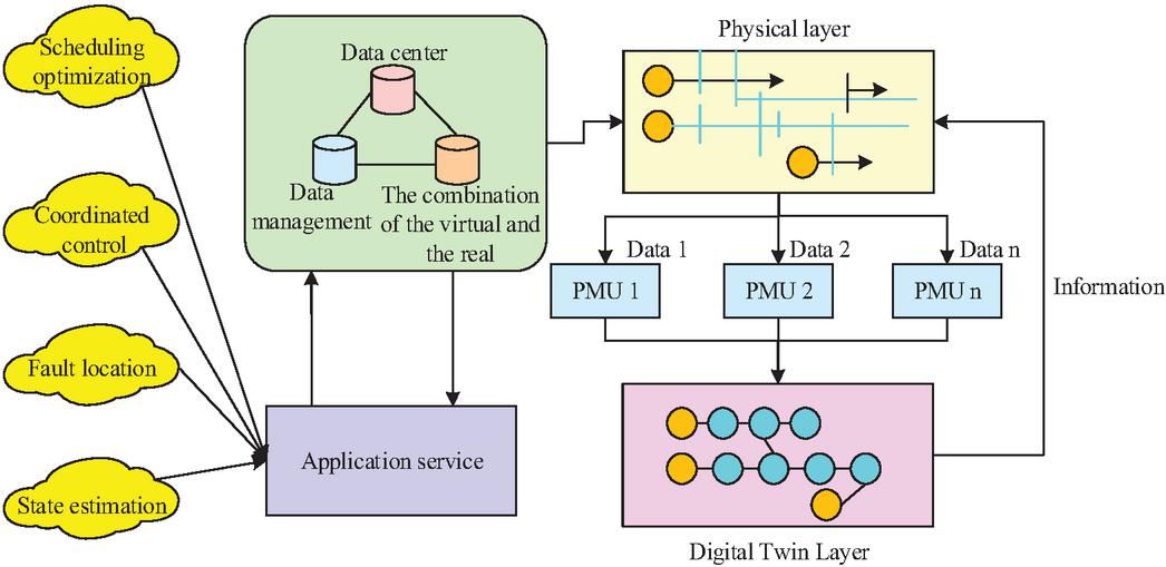
Figure 1 DT technology.

In Figure 1, the DT application framework of the DN presents a closed-loop architecture of physical, data and application three-layer collaboration. Each layer has independent technical attributes and forms an organic whole through data interaction. The physical layer is the foundation of the architecture. Its deployed sensing devices include distribution transformer temperature sensors, feeder current transformers and tower environmental monitoring terminals, which can realize millisecond-level multi-source data acquisition. The acquired data includes equipment operating status quantities, power quality parameters and environmental impact factors, providing a high-fidelity physical data source for the construction of the DT [13]. The temperature monitoring of the distribution transformer uses a thermodynamic model, as shown in Equation (1).

P_{loss} = I^{2} R + P_{core}

(1)

In Equation (1), $P_{loss}$ represents the total loss, $I$ is the current, $R$ is the resistance, and $P_{core}$ is the core loss. The feeder current transformer is based on the principle of electromagnetic induction, and its expression is shown in Equation (2).

I_{s} = \frac{I_{p}}{B}

(2)

In Equation (2), $I_{p}$ represents the primary current, $I_{s}$ represents the secondary current, and $B$ is the transformation ratio. The data acquisition layer constructs a reliable data channel between the physical world and the digital space through edge computing nodes and dedicated power communication networks. The DT layer transforms the component connection relationship of the physical power grid into a structural virtual model and realizes dynamic updating of model parameters through real-time data driving. Based on the high-fidelity simulation capability of the DT, the application service layer deeply integrates the functional modules such as scheduling optimization and fault location with the actual operation and maintenance needs of the DN [14]. Given that the DT model is difficult to effectively mine the spatial dependency relationship between components, the study introduces GCN to improve the DT model. GCN can identify features from non-Euclidean data and can characterize the topological connection relationship of DN components through the adjacency matrix (AM), realize the structured feature learning of the power grid operation status, and thus improve the situational awareness performance of the DT model [15]. The graph Laplace matrix is a core matrix in graph theory, which characterizes the topological structure and properties of the graph [16]. Each element $L_{i j}$ in the Laplace matrix $L$ is defined as shown in Equation (3).

L_{i j} = {\begin{matrix} \deg (v_{i}) & i = j \\ - 1 & i \neq j \\ 0 & otherwise \end{matrix}

(3)

In Equation (3), $\deg (v_{i})$ represents the degree of node $i$ , and $L_{i j} = - 1$ represents the condition that if $i \neq j$ and node $i$ is adjacent to node $j$ . The most commonly used matrix in GCN is the symmetric normalized Laplace matrix $L_{sym}$ , whose expression is shown in Equation (4).

L_{sym} = D^{- \frac{1}{2}} L D^{- \frac{1}{2}} = I - D^{- \frac{1}{2}} A D^{- \frac{1}{2}}

(4)

In Equation (4), $A$ is the AM of the graph, $D$ is the degree matrix (DM) of the graph, and $I$ is the identity matrix [17]. The architecture of the DN operation situation awareness model based on the improved DT model of GCN is shown in Figure 2.

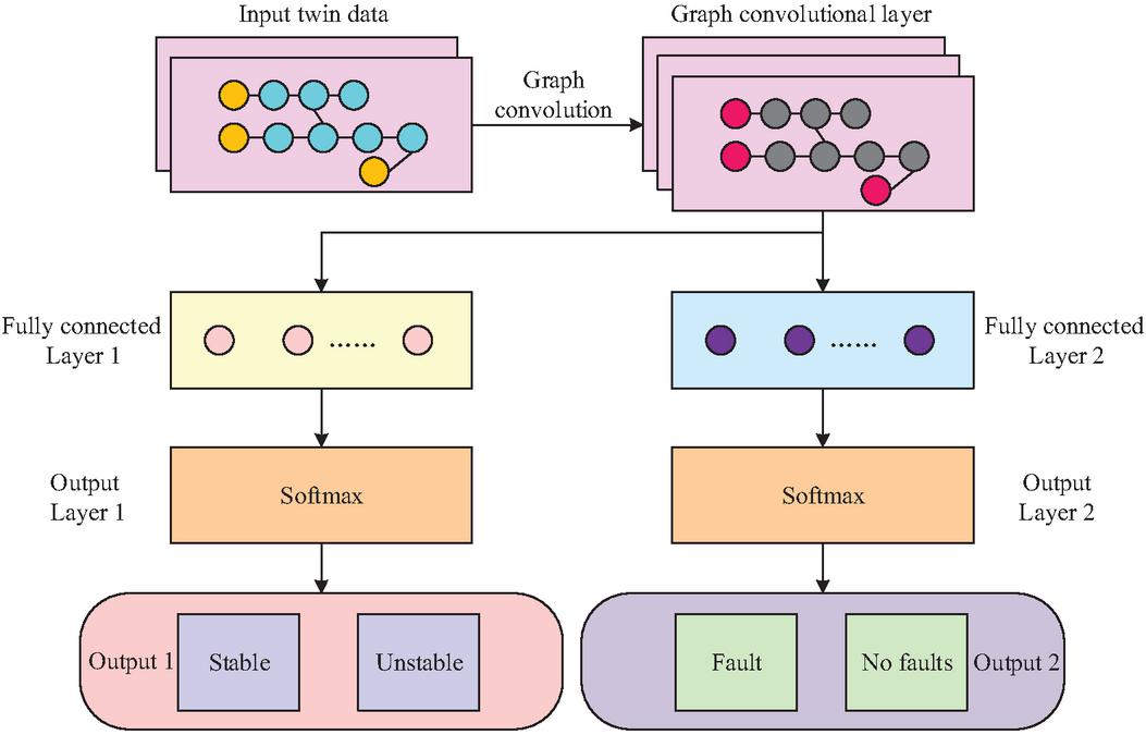
Figure 2 Architecture of DN operation situation awareness model based on GCN improved DT model.

As shown in Figure 2, the input layer receives the DN twin data and provides a high-dimensional input feature map for the model. The convolutional layer is the core feature extraction module. Based on the DN topology AM, the input data is fused with spatial features to explore the intrinsic relationship between the component operating status and topological association, and output a feature vector with topological awareness [18]. The node level feature vectors with strong topology awareness extracted by GCN are respectively fed into two structurally independent and parameter unshared fully connected branch networks. The stability prediction branch usually consists of 2–3 fully connected layers, and ultimately outputs a scalar through the Sigmoid activation function, representing the stability probability of the entire system or a specific region. The fault location branch adopts a fully connected network with a similar structure, and finally outputs a vector with the same dimension and number of nodes. Each node corresponds to a fault confidence level, which is normalized by the Softmax function. The node with the highest confidence level is determined as the fault source. Finally, the two sets of output layers output the DN operation stability assessment results and fault location results, respectively, to realize multi-task collaborative perception of the DN operation status. The model adopts a multi task joint loss function for end-to-end training, consisting of binary cross entropy loss for stability prediction and cross entropy loss for fault localization. Adam optimizer is used in training, and Dropout and early stopping strategies are employed to prevent overfitting.

2.2 DN Operation Fault Location

DNs are characterized by complex topologies and uneven deployment of measurement equipment. Relying solely on limited measurement data from key nodes to directly determine fault types and locations is prone to misjudgments or omissions due to incomplete measurement information. Therefore, it is necessary to accurately estimate the measurement status of all nodes in the topology using a model to provide complete data support for fault location. Considering the advantages of GCN in processing topology-related data, this study adopts a GCN-based SR (Super Resolution) model to estimate the measurement characteristics of all nodes in the DN. The fault location process for DN operation based on the improved DT model using GCN is shown in Figure 3.

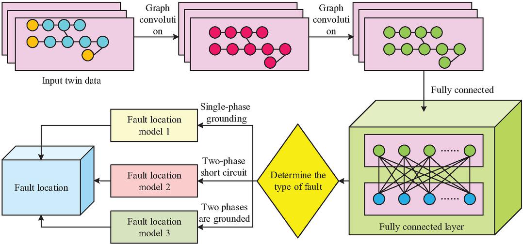
Figure 3 Fault localization process for DN operation based on GCN improved DT model.

As shown in Figure 3, the input key node measurement data is preprocessed through data cleaning, normalization, and topology mapping to generate full node feature twin data that matches the DN topology. This twin data is then input into the feature estimation module, which comprises two cascaded graph convolutional layers and an FCL. The preceding graph convolutional layer, based on the DN topology AM, mines the electrical correlation features between key nodes and non-measured nodes. The FCL completes feature dimension transformation and nonlinear fitting, ultimately outputting the estimation results of the actual node feature measurement values of the entire DN, filling the information gaps of non-measured nodes. The expression for the first graph convolutional layer is shown in Equation (5).

H^{(1)} = σ ({\tilde{D}}^{- \frac{1}{2}} \tilde{A} {\tilde{D}}^{- \frac{1}{2}} X W^{(0)})

(5)

In Equation (5), $H^{(1)}$ represents the output of the first GCN layer, $X$ represents the input feature matrix, $\tilde{A}$ represents the AM with added self-connections, $\tilde{D}$ represents the DM of $\tilde{A}$ , $W^{(0)}$ represents the trainable weight matrix (WM) of the first GCN layer, and $σ$ represents the activation function (AF). The expression for the second convolutional layer is shown in Equation (6).

H^{(2)} = σ ({\tilde{D}}^{- \frac{1}{2}} \tilde{A} {\tilde{D}}^{- \frac{1}{2}} H^{(1)} W^{(1)})

(6)

In Equation (6), the output of the second-layer GCN is $H^{(1)}$ , which represents the trainable WM of the second-layer GCN. Given the actual operational features of the DN, the study considers 1-phase grounding faults, 2-phase short-circuit faults, and 2-phase grounding faults, and constructs corresponding fault location sub-models. Finally, after determining the current fault category through the fault type identification module, the full node feature estimation results are passed to the matching fault location sub-model. The model accurately locates the fault location by comparing the changes in node electrical quantities before and after the fault. To address the insufficient robustness of traditional fault location methods under dynamic topology changes or measurement noise interference, this study introduces GAT to optimize the fault location task, building upon the previous DT model constructed based on GCN. Compared to GCN’s mechanism of equally weighting the features of neighboring nodes, GAT adaptively learns the contribution weights of different neighboring nodes to the target node through an attention mechanism, which can more accurately capture the electrical correlation features between key nodes and faulty nodes when a DN fault occurs. The fault location model based on GAT is shown in Figure 4.

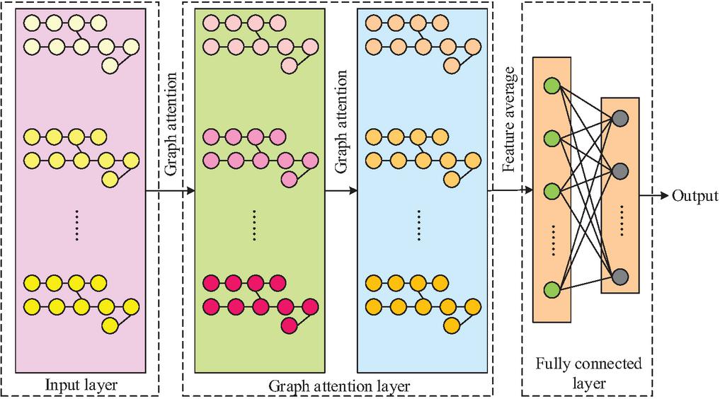
Figure 4 Fault localization model based on GAT.

In Figure 4, the model input layer receives the full-node electrical feature data output by the DT of the DN. The data passes through two cascaded graph attention layers. The first graph attention layer focuses on the node’s own features and the features of its immediate neighboring nodes, and calculates the attention coefficient to highlight the feature contribution of fault-related nodes. The second graph attention layer is grounded in the feature aggregation of the first layer. Then, the feature vectors output by the two graph attention layers are fused through the feature averaging module to eliminate the limitations of single-level feature aggregation. Finally, the fused feature vector is input to the FCL. In order to stabilize the learning process and capture information from different feature subspaces, GAT adopts multi-head attention and uses a splicing method in the intermediate layer to fuse features from different representation subspaces. The calculation formula is shown in Equation (7).

{\vec{h}}_{i}^{t} = ∥_{k = 1}^{K} σ (\sum_{j \in N (i)} α_{i j}^{k} W^{k} {\vec{h}}_{j}

(7)

In Equation (7), ${\vec{h}}_{i}^{t}$ represents the output feature vector of node $i$ after passing through the attention layer of this graph, $K$ represents the quantity of “heads” in the multi-head attention mechanism, $α_{i j}^{k}$ represents the normalized attention weight of node $j$ on node $i$ at the $k$ th attention head, $W^{k}$ represents the trainable linear transformation WM corresponding to the $k$ th attention head, and ${\vec{h}}_{j}$ represents the input feature vector of node $j$ . The model is trained in a supervised manner, and its loss function is the cross-entropy loss, as shown in Equation (8).

L^{'} = - \frac{1}{N} \sum_{i = 1}^{N} \sum_{c = 1}^{C} y_{i, c} \log ({\hat{y}}_{i, c})

(8)

In Equation (8), $L^{'}$ represents the loss value, $N$ is the total number of nodes in a training batch, $C$ is the total number of categories, $y_{i, c}$ is the true label, and ${\hat{y}}_{i, c}$ is the probability predicted by the model. The nonlinear mapping of multiple layers of neurons completes the mapping from fault features to fault location labels, ultimately outputting the specific number of the fault node in the DN, thus achieving precise fault location. Research on suppressing feature redundancy through collaborative design of feature extraction and model architecture. Embedding dropout layers in the GCN module to randomly mask invalid feature dimensions, and enhancing the directional extraction of electrical correlation core features based on the distribution network topology adjacency matrix to reduce irrelevant information interference; In the GAT module, the self attention mechanism is used to dynamically learn the weight allocation of neighboring nodes, allowing fault related nodes to receive higher attention. At the same time, a multi head attention mechanism is adopted to achieve differentiated extraction of multiple feature subspaces, effectively avoiding repeated representation of single dimensional features.

2.3 Operation Stability Analysis of DN

False data injection attack in power system is a network attack that takes advantage of the vulnerability in power system state estimation, tampers with measurement data, affects the control center’s judgment of the system state, and thus causes mis-scheduling or system collapse. Therefore, accurate detection of false data constitutes a vital part in securing the correctness of power grid situational awareness and maintain system stability. Considering that the DN operation data has significant temporal correlation, and the advantages of LSTM in capturing temporal data dependencies and suppressing noise interference, this study introduces LSTM to construct a false data injection detection model based on the improved DT model based on GCN, so as to realize the real-time discrimination of the authenticity of measurement data [19]. The stable operation process of DN based on LSTM algorithm is shown in Figure 5.

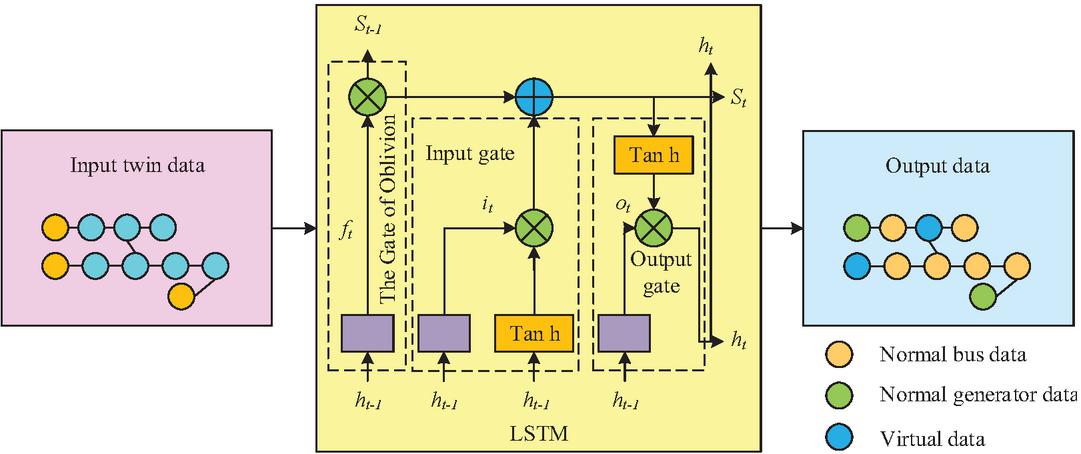
Figure 5 Stable operation process of DN based on LSTM.

As shown in Figure 5, the detection model adopts a two-layer LSTM network architecture. The input is the DN time series measurement data sequence, where $x_{t}$ represents the input vector at time step (TS) $t$ . At each TS $t$ , the LSTM network simultaneously receives the current input $x_{t}$ and the hidden state (HS) $z_{t - 1}$ of the previous TS $t - 1$ . Through the synergistic effect of the input gate (IG), forget gate (FG), cell state (CS) update and output gate (OG), the dynamic learning of time series features is completed [20]. Among them, the IG is used to control the update weight of the current input information $x_{t}$ , and its mathematical expression is shown in Equation (9).

i_{t} = σ (W_{x i} x_{t} + W_{z i} z_{t - 1} + b_{i})

(9)

In Equation (9), $W_{x i}$ and $W_{z i}$ are the WMs of the IGs corresponding to the input $x_{t}$ and the HS $z_{t - 1}$ , respectively, and $b_{i}$ is the IG bias term [21]. The FG is used to control the proportion of old information retained in the CS $c_{t - 1}$ of the previous TS, and its expression is shown in Equation (10).

f_{t} = σ (W_{x f} x_{t} + W_{z f} z_{t - 1} + b_{f})

(10)

In Equation (10), $W_{x f}$ and $W_{z f}$ are the weight matrices corresponding to the FG, and $b_{f}$ is the FG bias term; the degree of forgetting of old information is adjusted by the output value of $f_{t}$ . When a data mutation is detected, the output of the FG approaches 0, reducing the interference of abnormal old information on the current state [22]. Subsequently, the model uses candidate CSs, as shown in Equation (11).

{\tilde{c}}_{t} = \tanh (W_{x c} x_{t} + W_{z c} z_{t - 1} + b_{c})

(11)

In Equation (11), $\tanh$ is the hyperbolic tangent AF, which maps the value to the interval $[- 1, 1]$ to update the CS, thus obtaining the CS $c_{t}$ at the current TS. Finally, the OG $o_{t}$ controls the output of the CS to the HS, thus obtaining the current HS $z_{t}$ . The calculation formula of $o_{t}$ is shown in Equation (12).

o_{t} = σ (W_{x o} x_{t} + W_{z o} z_{t - 1} + b_{o})

(12)

In Equation (12), $W_{x o}$ represents the WM of the OG, and $b_{o}$ represents the bias term of the OG. Finally, the HS input classification layer is used to distinguish between normal and false injections of measurement data, providing a reliable data foundation for subsequent DN stability analysis and scheduling decisions.

3 Analysis of the Results of DN Operation Situation Perception Technology

3.1 Analysis of Fault Location Results of DN Operation Situation

To confirm the efficacy of the introduced model in DN fault location, the IEEE 37-bus system was used as the simulation object, and a simulation experimental environment was built using Matlab/Simulink. Integrate SimPowerSystems toolbox to build a distribution network simulation model, with a sampling frequency set to 50Hz and a data acquisition time step of 0.02 s, ensuring real-time and accurate data. The load level is measured in units, and a random sampling method is used to select load values within the range of 0.3 $\sim$ 1.0, covering three typical operating states of the distribution network: light load (0.3 $\sim$ 0.5), rated load (0.6 $\sim$ 0.8), and heavy load (0.9 $\sim$ 1.0). The proportion of experimental samples in each state is 1/3 to ensure the universality of the experimental results. The fault scenario design includes four typical types of faults in the distribution network: single-phase grounding fault, two-phase short-circuit fault, two-phase grounding short-circuit fault, and three-phase short-circuit fault. The fault occurrence time is randomly set within 1–10 seconds after the simulation starts, and the fault duration is fixed at 0.2 seconds. The fault resistance is selected as 0.05 $Ω$ (metallic short-circuit fault), 10 $Ω$ (conventional non-metallic fault), 25 $Ω$ (medium high resistance fault), and 1000 $Ω$ (high resistance grounding fault), covering the fault conditions of the distribution network comprehensively. For each typical fault type at each node in the IEEE 37-bus system, 100 independent data samples were generated, resulting in a dataset containing 14,800 samples. This dataset was divided into a training set (80%, 11,840 samples) and a test set (20%, 2,960 samples) using the industry-standard 8:2 ratio, for model parameter optimization and fault location performance verification, respectively. The confusion matrix of the proposed model’s fault location performance is shown in Figure 6.

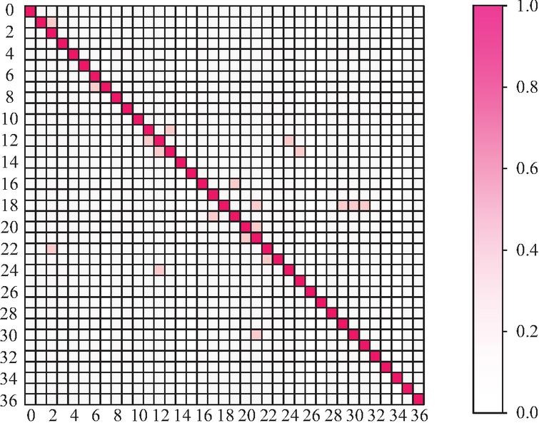
Figure 6 Confusion matrix of fault localization performance of the research model at IEEE37 nodes.

As shown in Figure 6, the fault location accuracy of the proposed model reached 97.2%, indicating that the proposed model could effectively identify fault types of different nodes and maintain high location accuracy under load fluctuation and fixed fault resistance conditions. To systematically evaluate the robustness of the introduced model under various fault resistance conditions, multiple sets of fault location test experiments were designed. The experiments selected four typical fault resistance values: 0.05 $Ω$ (simulating metallic short-circuit fault), 10 $Ω$ (conventional non-metallic fault), 25 $Ω$ (medium-high resistance fault), and 1000 $Ω$ (high resistance grounding fault) to cover common fault scenarios in DNs. Meanwhile, three core evaluation indicators were introduced: fault location accuracy, average location error, and fault location accuracy without jumps, to comprehensively quantify the model’s location performance. To fully highlight the superiority of the proposed GCN based improved digital twin model, in addition to selecting the traditional Graph Convolutional Neural Network (GCN) model and Random Forest (RF) model as the basic comparison algorithms, two more representative comparison algorithms have been added: one is LSTM, which is a typical time series modeling method that uses 18 dimensional feature inputs, 2-layer LSTM, and fully connected layer structure; The second is GAT, as an advanced graph model of GCN, which adopts a two-layer attention mechanism and sets the number of attention heads to 4. The optimizer, learning rate, training epochs, and other parameters of all machine learning comparison models are consistent with the proposed model to ensure fairness in comparison. The experimental results are shown in Table 1.

Table 1 Comparison of fault localization performance of various algorithms under various fault resistances

		Fault Localization	Average	Fault Localization
Fault	Model	Accuracy	Positioning Error	Zero Jump
Resistance	Type	(%)	(km)	Accuracy (%)
0.05 $Ω$	GCN	91.7	2.4	90.5
	RF	88.5	3.7	86.2
	LSTM	89.8	3.0	87.5
	GAT	93.4	1.8	92.1
	Ours	99.2	0.3	98.8
10 $Ω$	GCN	90.0	2.6	88.8
	RF	87.2	3.9	84.5
	LSTM	88.5	3.2	85.8
	GAT	92.1	2.0	90.7
	Ours	97.5	0.5	97.0
25 $Ω$	GCN	89.3	2.8	87.6
	RF	86.3	4.1	83.1
	LSTM	87.2	3.5	84.2
	GAT	91.5	2.2	89.9
	Ours	96.8	0.7	96.2
1000 $Ω$	GCN	87.6	3.1	85.3
	RF	84.6	4.4	81.8
	LSTM	85.7	3.8	82.9
	GAT	90.2	2.5	88.4
	Ours	95.1	1.0	94.5

As shown in Table 1, compared with the RF model, the proposed model improved the fault location accuracy by an average of 10.5% and reduced the average location error by 3.4 km. Furthermore, the fault location accuracy without jumps was significantly improved, indicating superior accuracy and stability under complex resistive conditions. Compared with the conventional GCN model, the fault localization accuracy of the proposed model is improved by 7.5%, and reduced the average location error by 2.1 km, demonstrating that the model’s ability to mine graph structure information and its efficiency in extracting fault features were both superior to the traditional GCN model. To evaluate the anti-interference capability of the proposed model in practical engineering scenarios, Gaussian white noise was added to the test set data, setting four signal-to-noise ratio conditions: 10 dB (strong noise), 20 dB (medium-strong noise), 30 dB (medium-weak noise), and 40 dB (weak noise). The fault location performance of the proposed model, GCN, and RF was compared, and the experimental numerical outcomes are presented in Figure 7.

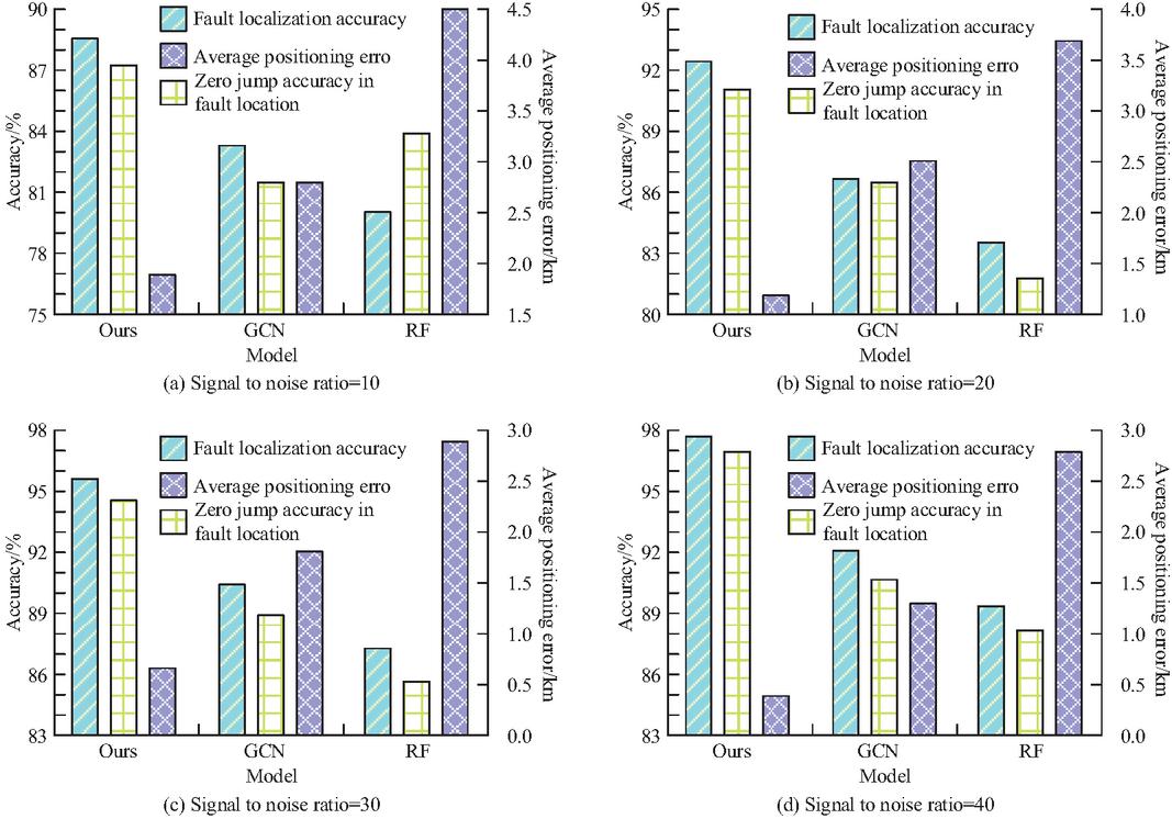
Figure 7 Numerical results of fault localization performance under different signal-to-noise ratios and noise effects.

Figure 7(a) indicates the numerical results of the model’s fault location performance under the 10dB operating condition. The fault location accuracy of the proposed model was 88.5%, which was 5.3% and 8.4% higher than that of GCN and RF, respectively; the average location error was 1.8 km, which was much lower than that of GCN. Figure 7(b) shows the numerical results of the model’s fault location performance under the 20 dB operating condition. Under the 20 dB operating condition, the fault location accuracy of the research model was improved to 92.3%, and the average location error was reduced to 1.2 km. Figure 7(c) shows the numerical results of the model’s fault location performance under the 30 dB operating condition. In the 30 dB low-noise environment, the location accuracies of the three models were 95.7%, 90.4%, and 87.2%, respectively, and the fault location accuracy without jumps of the proposed model reached 94.5%. Figure 7(d) shows the numerical results of the model’s fault location performance under the 40 dB operating condition. Under the 40 dB low-noise operating condition, the location accuracy of the proposed model was as high as 97.8%, while the location accuracy of RF was 89.3%. Furthermore, the proposed model achieved a non-jump accuracy of 96.9%, approaching 100% stable output.

3.2 Analysis of Stability Outcomes of DN Operation Situation

To verify the effectiveness of the introduced model in predicting stability in dynamic power DN scenarios, an experimental environment was built using the New England Test System, and a simulation model was constructed using PowerFactory software. Two data acquisition schemes were designed: first, two operating conditions were preset (stable and unstable), collecting core data such as bus voltage, current, and generator output; second, faults were set at the bus and generator ends, collecting transient fault data and location feature parameters. The total simulation time was 5 seconds, with a 0.1-second fault termination period after triggering to simulate a real-world scenario, ultimately obtaining 12,800 valid samples (6,500 stable samples and 6,300 unstable samples). Four-fold cross-validation was used, dividing the dataset into a 4:1 ratio: a training set (10,240 samples, 5,200 stable samples and 5,040 unstable samples) and a test set (2,560 samples). The test set was further divided into four subsets (640 samples each), with each subset having a stable/unstable sample ratio of approximately 1:1. Test set 1 contained 322 stable samples and 318 unstable samples; test set 2 contained 325 stable samples and 315 unstable samples; test set 3 contained 320 stable samples and 320 unstable samples; test set 4 contained 323 stable samples and 317 unstable samples, ensuring a balanced data distribution. The model used the bus as the analysis object to perform stability prediction, and the outcomes are presented in Figure 8.

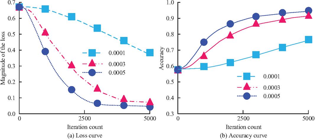
Figure 8 Stability prediction results of the bus used in the model.

Figure 8(a) shows the loss function of the bus used by the model for stability prediction. As shown in Figure 8(a), when the learning rate (LR)was set to 0.0001, the loss function did not fully converge even after 5000 iterations. When the LR was increased to 0.0003, the loss function converged after 4000 iterations. When the LR was further increased to 0.0005, the convergence speed was significantly accelerated, and convergence could be achieved in only 3000 iterations. Figure 8(b) shows the training accuracy of the bus used by the model for stability prediction. As shown in Figure 8(b), among different LR parameters, the model achieved the highest training accuracy of approximately 0.94 at 5000 iterations when the LR was 0.0005. To verify the stability prediction performance of the introduced model relying solely on generator mapping information, the study used generators as the analysis object and only used generator mapping information for training and prediction. The experimental outcomes are presented in Figure 9.

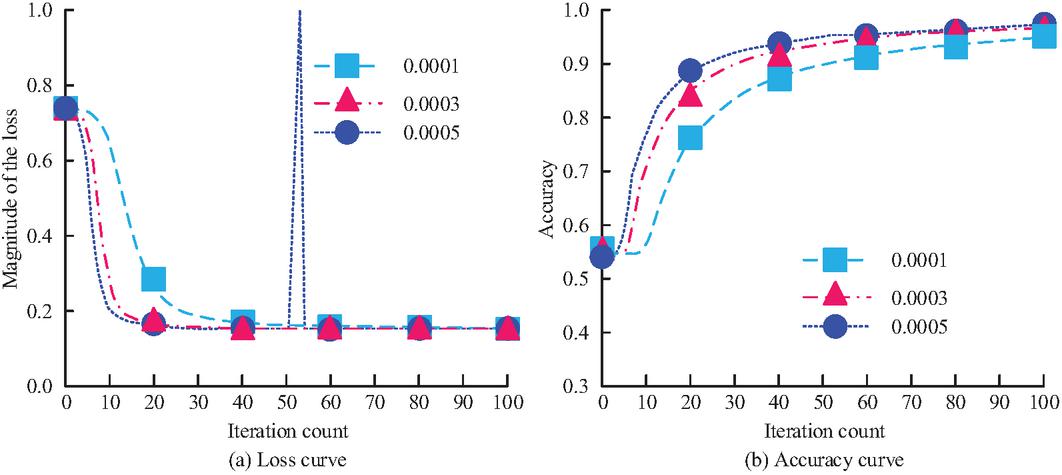
Figure 9 Stability prediction results of the generator used in the model.

Figure 9(a) shows the loss function of the generator used in the model for stability prediction. When the LR was set to 0.0005, the model reached convergence earliest at 20 iterations. However, the loss function fluctuated significantly around the 53rd iteration, indicating insufficient stability of the model training process at this LR. Figure 9(b) shows the training accuracy of the generator used in the model for stability prediction. After 100 iterations, the model training accuracy reached 0.98 at LRs of 0.0003 and 0.0005, significantly higher than the case with an LR of 0.0001. In summary, when the model relied solely on generator mapping information for stability prediction, an LR of 0.0003 was the optimal parameter choice, achieving high prediction accuracy while ensuring training stability. To further evaluate the stability of the proposed model, the study used three metrics – accuracy, recall, and F1 score – to comprehensively quantify the model’s prediction performance on three types of analysis objects: bus, generator, and all components (bus + generator). The outcomes are presented in Table 2.

Table 2 Stability prediction results of bus, generator, and all components on various test sets

/	Set 1	Set 2	Set 3	Set 4
Bus	Accuracy	99.20%	99.75%	99.95%	99.85%
	Recall	98.80%	99.50%	99.90%	99.70%
	F1 score	99.00%	99.62%	99.92%	99.77%
Generator	Accuracy	99.10%	98.50%	98.80%	99.80%
	Recall	98.90%	98.30%	98.60%	99.70%
	F1 score	99.00%	98.40%	98.70%	99.75%
All components	Accuracy	99.50%	99.90%	99.85%	99.80%
	Recall	99.40%	99.85%	99.80%	99.75%
	F1 score	99.45%	99.87%	99.82%	99.77%

As shown in Table 2, the three metrics of the bus performed robustly across the four test sets, with accuracy exceeding 99% for all sets. Test set 3 peaked at 99.95%, while test set 1 had the lowest accuracy at 99.20%. Test set 3 had the highest recall and F1 score, at 99.90% and 99.92%, respectively. The generator’s accuracy varied between 98.50% and 99.80%, with a fluctuation range of 1.3%. Test set 2 performed the weakest, with a recall of 98.30% and an F1 score of 98.40%. Test set 4 performed the best, with a recall of 99.70% and an F1 score of 99.75%. The bus and generator components exhibited a dual advantage of high precision and low fluctuation, with accuracy exceeding 99.50% for all sets, peaking at 99.90% in test set 2. The fluctuation across the four test sets was only 0.4%; the fluctuation ranges for recall and F1 score were both less than 0.5%. From this, it can be seen that the proposed model exhibits high accuracy and stability in bus, generator, and full component analysis, and the full component analysis mode of bus $+$ generator has the best performance, laying a core performance foundation for practical engineering applications. To evaluate the robustness of the model under data integrity breach scenarios, the study set a false data injection detection false judgment rate of 2%, and injected 2% false data into the original test data (12,544 normal groups and 256 false groups). False data is a typical false data injection attack model based on the state estimation scenario of the distribution network, constructed to simulate real cyber attack scenarios. When generating, based on the IEEE test system topology and electrical constraints, calculate the benchmark disturbance vector that meets measurement consistency, and then make differential adjustments for steady-state (Test A) and transient (Test B). There are two types of scenarios: steady-state operating conditions (Test A) and transient processes (Test B) (1280 sets each, including 26 sets of false data). The superposition of steady-state data and subtle disturbances strongly correlated with electrical quantities such as voltage and power; Transient data simulates the temporal abrupt changes during faults, with disturbances dynamically changing as the fault evolves. Finally, 2% of false data was mixed into the original set through random sampling to ensure that the attack data has both concealment and scene adaptability. The outcomes are presented in Table 3.

Table 3 Stability prediction results containing 2% erroneous data

Test Type	Precision	Recall	F1 Score	Accuracy
Bus test A	98.65%	98.40%	98.52%	98.55%
Bus test B	98.80%	98.55%	98.67%	98.70%
Generator test A	98.35%	98.10%	98.22%	98.25%
Generator test B	98.50%	98.25%	98.37%	98.40%
Total test A	98.95%	98.75%	98.85%	98.90%
Total test B	99.05%	98.85%	98.95%	99.00%

As shown in Table 3, despite the 2% injection of spurious data, the precision, recall, F1 score, and accuracy of all test schemes remained above 98%. The lowest accuracy was 98.25% for generator test A, and the highest was 99.00% for overall test B, with an overall fluctuation of only 0.75%. The lowest F1 score was 98.22% for generator test A, and the highest was 98.95% for overall test B. This demonstrated that the model could effectively capture the core characteristics of power grid stability even under spurious data interference, and its anti-interference capability met the reliability requirements of actual DN operation. To enhance the credibility of the GCN enhanced digital twin model, interpretability research is conducted from three aspects: quantification of key node contributions, analysis of line correlation weights, and verification of actual fault scenarios. The study adopts a combination of GCN layer weight visualization and node gradient significance analysis. By extracting the weight matrix of the last layer GCN of the model, the weight coefficients of each node feature on the stability prediction results of the output layer are calculated; At the same time, the gradient rise method is used to solve the gradient values of the model output on the input features of each node. The larger the absolute value of the gradient, the more significant the impact of the node on the prediction results. The analysis results of key nodes and line contributions are shown in Table 4.

Table 4 Analysis results of key nodes and line contributions

Node	Node	Contribution	Core	Line
Type	Number	Based Index	Associated Lines	Association Weight
Bus	#2	0.92	L2-1, L2-5	0.89, 0.87
	#5	0.88	L5-2, L5-8	0.85, 0.83
	#8	0.85	L8-5, L8-10	0.82, 0.80
Generator	#1	0.90	L1-2	0.91
	#3	0.86	L3-4	0.88
	#6	0.83	L6-7	0.84

According to Table 4, the contribution index of bus # 2 identified by the pre fault model is 0.92, and the associated weight of L2-1 line is 0.91; 0.05 seconds after the fault occurred, the voltage of the # 2 bus dropped sharply by 15%. The model quickly captured the power mutation characteristics of the L2-1 line through the GCN layer, and the contribution index of the # 1 generator instantly increased to 0.95, triggering a stability warning. After 0.08 seconds of fault removal, the voltage of the # 2 bus returned to 90% of the rated value, and the weight coefficients of the # 2 bus and L2-1 line in the model synchronously fell back to the normal range, and the warning was lifted. The decision focus of the model throughout the entire process perfectly matched the fault evolution path, further confirming the rationality of interpretability analysis. The interpretability analysis shows that the stability prediction decision of the GCN enhanced digital twin model is not a black box operation. The contribution ranking of its key nodes/lines is highly consistent with the physical laws of the power system, and the core decision basis is clear and traceable, significantly improving the credibility and acceptance of the model in engineering applications.

4 Conclusion

To address the challenges of operational situation awareness arising from the high proportion of renewable energy integration and diverse load interactions in DNs of new power systems, this study proposed an improved DT model based on GCN. Experimental verification and performance analysis were conducted. The study found that in fault location tasks, the introduced model achieved a location accuracy of 97.2% in the IEEE 37-bus system test. Facing different fault resistances ranging from 0.05 $Ω$ to 1000 $Ω$ and noise interference ranging from 10 dB to 40 dB, its location accuracy consistently outperformed GCN and random forest algorithms, with a minimum average location error of only 0.3 km. Its anti-interference and robustness met engineering requirements. In stability analysis and spurious data detection tasks, after fusing bus and generator data, the model achieved a stability prediction accuracy exceeding 99.5%. Even after injecting 2% spurious data, its performance remained above 98%, effectively ensuring the accuracy and security of power grid situation awareness. In summary, this research provides a feasible technical path for the digital operation and maintenance of DNs under new power systems. In addition, this technology can be transferred to scenarios such as active distribution networks and microgrids, adapting to the situational awareness needs under high penetration rates of distributed power sources. The fusion logic of GCN and digital twins can also be extended to fields such as transmission network fault diagnosis and comprehensive energy system optimization scheduling, providing technical references for the full chain digital upgrade of new power systems and further expanding the application boundaries and academic influence of research. However, the proposed model suffers from high complexity. Future research could further optimize the model’s lightweight design, such as based on the topological partitioning characteristics of the distribution network, using a federated learning framework to distribute computing pressure, deploying complete models only at key nodes, and sharing simplified feature extraction modules with non key nodes to improve real-time response capabilities in large-scale power grids.

Acknowledgement

This research is supported by the National Natural Science Foundation of China:Research on the fundamental theory and method of digital twin of new power distribution system (U22B2096).

References

[1] Li Z, Xu Y, Wang P, Xiao G. Restoration of a multi-energy distribution system with joint district network reconfiguration via distributed stochastic programming [J]. IEEE Transactions on Smart Grid, 2023, 15(3): 2667–2680. DOI: 10.1109/TSG.2023.3317780.

[2] Sheta A N, Sedhom B E, Pal A, El M M S, Eladl A A. Stability-constrained settings of directional overcurrent relays with shifted user-defined characteristics for distribution networks with ders [J]. IEEE Transactions on Power Delivery, 2024, 39(4): 2401–2413. DOI: 10.1109/TPWRD.2024.3403921.

[3] Ebrahimi H, Yazdaninejadi A, Golshannavaz S. Transient stability enhancement in multiple-microgrid networks by cloud energy storage system alongside considering protection system limitations [J]. IET Generation, Transmission & Distribution, 2023, 17(8): 1816–1826. DOI: 10.1049/gtd2.12539.

[4] Mishra A, Tripathy M, Ray P. A survey on different techniques for distribution network reconfiguration [J]. Journal of Engineering Research, 2024, 12(1): 173–181. DOI: 10.1016/j.jer.2023.09.001.

[5] Heluany J B, Gkioulos V. A review on digital twins for power generation and distribution [J]. International Journal of Information Security, 2024, 23(2): 1171–1195. DOI: 10.1007/s10207-023-00784-x.

[6] Tang F, Luo L, Guo Z, Li Y, Zhao M, Kato N. Semi-distributed network fault diagnosis based on digital twin network in highly dynamic heterogeneous networks [J]. IEEE Transactions on Mobile Computing, 2024, 24(5): 3979–3992. DOI: 10.1109/TMC.2024.3519576.

[7] Ebtia A, Ghafouri M, Debbabi M, Kassouf M, Mohammadi A. Power distribution network topology detection using dual-graph structure graph neural network model [J]. IEEE Transactions on Smart Grid, 2024, 16(2): 1833–1850. DOI: 10.1109/TSG.2024.3512457.

[8] Madbhavi R, Natarajan B, Srinivasan B. Graph neural network-based distribution system state estimators [J]. IEEE Transactions on Industrial Informatics, 2023, 19(12): 11630–11639. DOI: 10.1109/TII.2023.3248082.

[9] Nguyen B L H, Vu T V, Nguyen T T, Panwar M, Hovsapian R. Spatial-temporal recurrent graph neural networks for fault diagnostics in power distribution systems [J]. IEEE Access, 2023, 11(1): 46039–46050. DOI: 10.1109/ACCESS.2023.3273292.

[10] Meng Q, Tong X, Hussain S, Luo F, Zhou F, He Y, Li B. Enhancing distribution system stability and efficiency through multi-power supply startup optimization for new energy integration[J]. IET Generation, Transmission & Distribution, 2024, 18(21): 3487–3500. DOI: 10.1049/gtd2.13299.

[11] Pirouzi S, Zadehbagheri M, Behzadpoor S. Optimal placement of distributed generation and distributed automation in the distribution grid based on operation, reliability, and economic objective of distribution system operator[J]. Electrical Engineering, 2024, 106(6): 7899–7912. DOI: 10.1007/s00202-024-02458-w.

[12] Guo M F, Liu W L, Gao J H, Chen D Y. A data-enhanced high impedance fault detection method under imbalanced sample scenarios in distribution networks [J]. IEEE Transactions on Industry Applications, 2023, 59(4): 4720–4733. DOI: 10.1109/TIA.2023.3256975.

[13] Cao H, Zhang D, Yi S. Real-Time Machine Learning-based fault Detection, Classification, and locating in large scale solar Energy-Based Systems: Digital twin simulation [J]. Solar Energy, 2023, 251(1): 77–85. DOI: 10.1016/j.solener.2022.12.042.

[14] Khan M M S, Giraldo J, Parvania M. Real-time cyber attack localization in distribution systems using digital twin reference model [J]. IEEE Transactions on Power Delivery, 2023, 38(5): 3238–3249. DOI: 10.1109/TPWRD.2023.3296312.

[15] Fan S, Wang X, Shi C, Cui P, Wang B. Generalizing graph neural networks on out-of-distribution graphs [J]. IEEE Transactions on Pattern Analysis and Machine Intelligence, 2023, 46(1): 322–337. DOI: 10.1109/TPAMI.2023.3321097.

[16] Gao M, Yu J, Yang Z, Zhao J. A physics-guided graph convolution neural network for optimal power flow [J]. IEEE Transactions on Power Systems, 2023, 39(1): 380–390. DOI: 10.1109/TPWRS.2023.3238377.

[17] Vatter J, Mayer R, Jacobsen H A. The evolution of distributed systems for graph neural networks and their origin in graph processing and deep learning: A survey [J]. ACM Computing Surveys, 2023, 56(1): 1–37. DOI: 10.1145/3597428.

[18] Wang Y, Fu W, Zhang X, Zhen Z, Wang F. Dynamic directed graph convolution network based ultra-short-term forecasting method of distributed photovoltaic power to enhance the resilience and flexibility of distribution network [J]. IET Generation, Transmission & Distribution, 2024, 18(2): 337–352. DOI: 10.1049/gtd2.12963.

[19] Kammoun M, Kammoun A, Abid M. LSTM-AE-WLDL: Unsupervised LSTM auto-encoders for leak detection and location in water distribution networks [J]. Water Resources Management, 2023, 37(2): 731–746. DOI: 10.1007/s11269-022-03397-6.

[20] Raghuvamsi Y, Teeparthi K. Distribution system state estimation with Transformer-Bi-LSTM-based imputation model for missing measurements [J]. Neural Computing and Applications, 2024, 36(3): 1295–1312. DOI: 10.1007/s00521-023-09097-5.

[21] Guha D, Chatterjee R, Sikdar B. Anomaly detection using LSTM-based variational autoencoder in unsupervised data in power grid[J]. IEEE Systems Journal, 2023, 17(3): 4313–4323. DOI: 10.1109/JSYST.2023.3266554.

[22] Liu K, Sheng W, Li Z, Liu F, Liu Q, Huang Y, Li Y. An energy optimal schedule method for distribution network considering the access of distributed generation and energy storage [J]. IET Generation, Transmission & Distribution, 2023, 17(13): 2996–3015. DOI: 10.1049/gtd2.12855.

Biographies

Hao Bai (July 1987–), male, graduated from Huazhong University of Science and Technology with a PhD in Electrical Engineering. After graduation, I worked as a senior engineer at Southern Power Grid Science Research Institute Co., Ltd. My current research direction is engaged in the planning and operation of distribution networks.

Wei Li (October 1993–), male, graduated from Tsinghua University with a master’s degree in Electrical Engineering. After graduation, I worked as an intermediate engineer at Southern Power Grid Science Research Institute Co., Ltd. My current research direction is engaged in the operation and control of distribution networks.

Yipeng Liu (October 1998–), male, graduated from Wuhan University with a master’s degree in Electrical Engineering. After graduation, I worked as an engineer at Southern Power Grid Science Research Institute Co., Ltd. My current research direction is engaged in the operation and simulation of distribution networks.

Distributed Generation & Alternative Energy Journal, Vol. 41_2, 301–326
doi: 10.13052/dgaej2156-3306.4123
© 2026 River Publishers