Research on Intelligent Control Technology for Cooperative Game Implementation in Source-Grid-Load-Storage Systems Based on Reinforcement Learning
Jinzhong Li1,*, Yuguang Xie1, Wei Ma1 and Kun Huang2
1State Grid Anhui Electric Power Co., Ltd. Electric Power Research Institute, Hefei, Anhui, 230601, China
2Hefei Zhongke Brain Intelligence Technology Co., Ltd., Hefei, Anhui, 230601, China
Email: tgzhuanyong202309@163.com; 981779186@qq.com; Yuguang202321@163.com; 95662479@qq.com; Wei202532@163.com; 16117385@bjtu.edu.cn; Huang202521@163.com; huangkun@leinao.ai
*Corresponding Author
Received 22 November 2025; Accepted 12 January 2026
Abstract
As the penetration rate of renewable energy sources such as wind and solar power continues to rise, coordinated control among multiple entities including generation, transmission, load and storage has become crucial for ensuring the economic efficiency and security of power systems. However, the uncertainty of renewable energy output, the multi-period coupling characteristics of flexible resources, and the inconsistency of benefits among entities make it challenging for traditional optimization methods to simultaneously address real-time responsiveness, robustness, and fairness. To address this, this paper proposes an intelligent control method for power generation, grid, load, and storage that integrates Proximal Policy Optimization (PPO) with cooperative game theory. First, a Markov decision model suitable for multi-source, multi-load systems is constructed. The continuous action space of flexible resources enables coordinated control of thermal power, energy storage, and adjustable loads. Subsequently, a penalty for deviation from cooperative payoffs is embedded in the reward function, ensuring that policy optimization simultaneously satisfies overall economic efficiency and inter-agent profit coordination requirements. Multi-scenario simulations on IEEE 33-node and IEEE 30-node systems demonstrate that this method achieves rapid and stable convergence, significantly reduces operational costs, smooths power fluctuations, and maintains sustainable SOC for energy storage. Compared to conventional methods, it exhibits stronger robustness and higher cooperative incentive effects under uncertain conditions.
Keywords: Grid-load-storage coordination, deep reinforcement learning, proximal policy optimization (PPO), cooperative games, uncertainty scheduling, intraday rolling optimization, renewable energy integration.
1 Introduction
As the global energy structure continues its transition toward clean and low-carbon sources, the penetration rate of renewable energy such as wind and solar power generation in power systems is rapidly increasing [1, 2]. Due to their inherent intermittency, randomness, and unpredictability, the high proportion of renewable energy integration poses unprecedented operational challenges to traditional power systems, which have long been centered on the principle of “generation following load.” These challenges include difficulties in power balancing, increased demand for reserve capacity, reduced grid safety margins, and large-scale curtailment of wind and solar power [3]. Concurrently, the rapid development of user-side resources, the continuous decline in energy storage costs, and the widespread adoption of communication technologies have driven the power system’s evolution from a unidirectional energy flow system dominated by generation to a new configuration featuring deep coupling among multiple entities, including generation, grid, load, and storage, and bidirectional flow of both energy and information. A vast array of flexible resources, including distributed PV, distributed wind power, controllable loads, and energy storage devices, are emerging as crucial forces supporting renewable energy integration and system resilience [4, 5]. This study focuses on designing and optimizing a multi-objective function for a community smart DC micro-grid using a hybrid system of photovoltaic, wind, and biogas-based IC engine generators, optimized through particle swarm optimization (PSO). The objectives are to maximize power availability and minimize system cost by prioritizing renewable generation to efficiently supply the DC bus [6].
However, this complex system composed of multiple resource categories exhibits typical characteristics of high dimensionality, strong coupling, and multi-temporal and spatial scales. The integration of renewable energy sources has increased the need for new technologies to manage issues like variability and intermittency. The coupling of generation, grid, storage, and load introduce new complexities, requiring advanced coordination methods to manage their interactions effectively. These interconnected systems must be dynamically optimized to account for real-time fluctuations and uncertainties in renewable energy generation. Innovative coordination solutions, such as cooperative game theory and reinforcement learning, are essential for achieving efficient and stable operation. Solutions such as energy storage demand response and predictive analytics are being used more to improve grid stability and support renewable energy use. These technologies are key to creating a more flexible and reliable power system that can handle large-scale renewable energy. Significant differences exist among its internal entities in operational objectives, cost structures, and regulatory capabilities, making it difficult for traditional centralized, deterministic dispatch models to maintain efficiency, economy, and stability under uncertain scenarios [7]. Therefore, achieving efficient coordinated control of generation, grid, load, and storage resources under high renewable energy penetration, while establishing sustainable and incentivized cooperative relationships among multiple entities, has become a critical scientific challenge and engineering bottleneck in building the new power system. A major gap in traditional methods is their inability to effectively coordinate multiple agents under high uncertainty in real-time power system operations. These models often overlook the diverse incentives of individual entities, leading to inefficiencies and suboptimal performance. Existing models often struggle to manage the dynamic and uncertain aspects of renewable energy generation. The challenge lies in their inability to effectively coordinate generation, grid, storage, and load under varying conditions. These systems face difficulties in providing real-time solutions, especially when dealing with the unpredictability of renewable sources like wind and solar. However, achieving these objectives remains fraught with significant challenges. First, the uncertainty of wind and solar power generation exhibits strong randomness and multi-scale coupling characteristics spanning hours, minutes, and even seconds. Traditional deterministic dispatch struggles to accurately capture their statistical distributions, while robust optimization often yields overly conservative solutions [8, 9]. Scenario-based methods, though capable of expressing uncertainty, rely on large-scale scenario generation and reduction, making them unsuitable for real-time solution demands in intraday rolling dispatch. Second, the joint dispatch of generation, grid, load and storage involve multiple non-convex coupled constraints: ramping constraints and start-stop logic for thermal units, SOC dynamics and nonlinear charge/discharge efficiency for energy storage systems, flexible time windows and user comfort for adjustable loads, and voltage and power flow constraints for the grid [10]. This creates a complex optimization problem with high-dimensional continuous decision variables. While traditional MILP/MINLP methods can approximate some nonlinearities, their computational complexity escalates sharply with increasing system scale and frequent state predictions, making them unsuitable for high-frequency rolling optimization. Kumar et al. investigated performance balancing between wind and solar energy systems and their environmental benefits by analysing hybrid renewable outputs and clean-energy enhancement strategies, focusing on efficiency and emission reduction. Elements of hybrid wind–solar integration, especially balancing variable renewable outputs and environmental performance metrics, were adapted into the proposed work’s source–grid–load–storage coordination model to improve renewable dispatch decisions under uncertainty. The integration improved grid flexibility, reduced renewable intermittency impact and enhanced operational reliability in real-time control environments [11].
Furthermore, inherent differences exist among multiple entities in terms of operational costs, risk preferences, regulatory capabilities, and revenue acquisition. Without reasonable revenue coordination and incentive mechanisms, entities such as energy storage, controllable loads, and renewable power generation may lack motivation to actively participate in system regulation [12, 13]. This could even lead to perverse incentives, dispatch games, or resource non-cooperation, severely undermining overall regulatory effectiveness. While existing cooperative and non-cooperative game-theoretic approaches can partially describe interactions among entities, they often struggle to deeply integrate with the physical constraints of power systems and maintain strategy stability during multi-period, multi-scenario rolling optimization.
Against this backdrop, Deep Reinforcement Learning (DRL) has garnered significant attention due to its ability to autonomously learn strategies through interaction with the environment within high-dimensional continuous state spaces. Recent research demonstrates DRL’s strong adaptability and generalization capabilities in complex energy system control [14, 15]. By directly outputting action policies without solving large-scale mathematical optimization problems, DRL is particularly well-suited for rolling optimization applications in energy systems. However, existing DRL scheduling research still exhibits significant shortcomings. For instance, it often lacks modeling of multi-agent cooperative relationships, with reward functions primarily focused on single-cost optimization without incorporating cooperative benefit distribution mechanisms. Most studies fail to simultaneously consider the coupled characteristics of the entire generation-grid-load-storage chain [16, 17]. Strategy stability and interpretability remain weak. Most models are validated only in simplified scenarios, lacking system-level simulation verification in typical distribution grids or hybrid transmission-distribution systems. Furthermore, when systems exhibit multi-scale uncertainties, DRL remains prone to issues such as slow convergence, significant oscillations, or strategy degradation. Therefore, there is an urgent need to develop an intelligent control method that can express cooperative relationships among multiple agents (generation, grid, load, and storage) while adapting to high-dimensional stochastic environments and meeting real-time rolling scheduling requirements [18, 19].
Based on the above issues, this paper proposes a collaborative intelligent dispatch method for source-grid-load-storage systems that integrates reinforcement learning and cooperative game theory (RL-Cooperative Dispatch Framework). This method first constructs a Markov Decision Process (MDP) model applicable to the generation-grid-load-storage system. Its state space incorporates load forecasts, renewable energy forecasts and actual output, energy storage State of Charge (SOC), previous-period unit status, and grid operational measurements, thereby achieving a unified characterization of uncertainties across different time scales. By incorporating cooperative game theory within the MDP framework, it ensures that the reward structure incentivizes joint optimization, leading to enhanced stability, lower operational costs and improved overall performance, even in the face of high uncertainty and dynamic system conditions.
2 Near-Real-Time Coordinated Dispatching Mechanism
2.1 Short-Term Optimization Strategy Based on Rolling Time Windows
With the growing penetration of renewable energy, power system scheduling has gradually shifted from static, plan-based management to dynamic and continuous optimization. To maintain system stability under rapidly changing load levels and variable wind–solar generation, system operators generally adopt a two-layer architecture consisting of day-ahead planning and intraday adjustment. In this framework, the day-ahead layer formulates the overall operating plan over a longer time horizon, while the intraday layer performs fine-grained updates to reflect short-term changes [20, 21]. Integrating Demand Response (DR) programs with generation and storage resources enhances both flexibility and economic efficiency in the dispatch strategy. By dynamically adjusting consumption patterns in response to price signals or grid conditions, DR programs provide an additional tool for balancing supply and demand, reducing the need for reserve capacity and curtailment of renewable energy. Optimizing this integration ensures that both economic goals and system reliability are met efficiently, especially during periods of high variability in renewable energy generation.
In the day-ahead stage, the scheduling model typically spans a full 24-hour period with an hourly time resolution. The rolling time window strategy ensures that the operational plan is continuously updated to reflect real-time changes in load and renewable generation. As new data becomes available, the system adjusts the schedule in short intervals, allowing for quick adaptation to unexpected fluctuations. This dynamic approach improves grid stability and maximizes renewable energy utilization by recalibrating dispatch decisions to meet current conditions. It determines the on/off status of controllable generating units and establishes their baseline output trajectories, forming the system’s initial operational blueprint [22]. Once the system enters the intraday stage, operators use updated meteorological forecasts, short-term load predictions, and real-time measurements to reassess the available renewable generation and expected demand variations. Based on this information, they revise the day-ahead output schedules as needed. The intraday optimization horizon is significantly shorter, usually a few hours, and employs minute-level resolution to enable frequent recalibration.
The core principle of intraday rolling optimization is to maintain scheduling decisions closely aligned with the latest system conditions through a continuously advancing optimization window. As each update is performed, the system can promptly detect sudden load changes, forecast deviations in wind and solar output, and any equipment irregularities. By rapidly coordinating controllable generators, energy storage systems, and adjustable loads, the dispatch strategy compensates for these deviations. This mechanism enables ongoing correction and dynamic adaptation, ensuring that the power grid maintains adequate security margins while improving operating economy and enhancing renewable energy utilization in the face of uncertainty (see Figure 1).
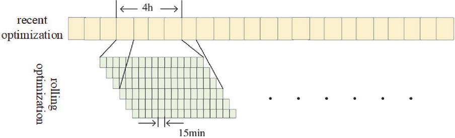
Figure 1 Intraday rolling optimization schematic diagram.
2.2 Mathematical Formulation of Rolling Intraday Coordinated Scheduling
With the increasing penetration of renewable energy, the share of conventional thermal and hydropower units, traditionally responsible for providing stable supply, continues to decline. As a result, the system’s inherent flexibility becomes insufficient to fully accommodate the variability and intermittency of renewable generation. In the context of new-type power systems, adjustable loads and energy storage have emerged as essential flexible resources. Building on the analysis in the previous chapter, this section develops a source–grid–load–storage intraday coordinated scheduling model in which both load curtailment and energy storage participate. The objective is to achieve efficient system operation and cost-optimal dispatching. A 4-hour rolling optimization window is adopted to update decisions continuously [23].
(1) Objective Function
The goal of the optimization model is to minimize the aggregate operating cost of all flexible resources within the scheduling horizon, including thermal generation costs, energy storage operating costs, and load adjustment costs. The uncertainty in renewable energy generation, driven by its intermittent nature, introduces significant challenges for grid stability. This uncertainty can cause power imbalances and necessitate real-time adjustments to balance supply and demand, often resulting in voltage instability or even grid failure. Managing this uncertainty is key to ensuring the reliable integration of renewable energy into the grid. The objective function is expressed as:
| (1) |
where: : set of thermal generating units; : set of energy storage systems; : set of adjustable loads; : set of discrete time steps within the intraday scheduling horizon.
Variables:
• : Power output of thermal generating unit at time step .
• : Charging power of energy storage system at time step .
• : Discharging power of energy storage system at time step .
• : Load adjustment (curtailment or shifting) for adjustable load at time step .
Cost Functions:
• : Operating cost of thermal generating unit as a function of its power output at time step .
• : Operating cost of energy storage system es based on its charging and discharging power at time step .
• : Cost associated with load adjustment (curtailment or shifting) for adjustable load at time step .
(a) Cost of Thermal Generating Units The operating cost of each thermal unit is modeled as a quadratic function:
| (2) |
where denote the unit’s cost coefficients.
• : The operating cost of thermal unit at time , which is typically measured in monetary units (e.g., dollars, euros) for the amount of power produced.
• : The power output of thermal unit at time , measured in units of power (e.g., megawatts, MW).
• : The quadratic coefficient that represents how the cost increases as the power output increases. It captures the non-linear relationship between power output and cost. A positive value of means that the cost increases more rapidly as power output increases.
• : The linear coefficient that represents the linear increase in cost with respect to the power output. It accounts for the basic operating costs that grow linearly with power production.
• : The constant coefficient, which represents the fixed or baseline cost of operating the thermal unit, regardless of the power output. This can include fixed maintenance costs, startup costs, or other overhead.
(b) Cost of Energy Storage Operation Energy storage incurs costs associated with charging/discharging losses and degradation. Its operating cost is modeled linearly:
| (3) |
Where and are charging and discharging power, respectively; and are the corresponding cost coefficients.
(c) Cost of Adjustable Load Regulation The cost associated with load reduction or shifting is represented using a penalty factor:
| (4) |
where denotes the load adjustment amount and is the penalty coefficient. In the context of demand response (DR) programs, customer-side incentives, such as dynamic pricing, rebates, or peak-time rebates, can be introduced to encourage load shifting or reduction. These incentives provide consumers with financial rewards or reduced rates for adjusting their energy usage during high-demand periods or in response to real-time grid conditions. By integrating DR programs, the system can improve coordination between the grid and the customer, enhancing the overall efficiency and flexibility of the energy distribution. These programs can also support grid stability by reducing peak load, smoothing out demand fluctuations, and ensuring better alignment between generation and consumption patterns.
(2) System Constraints for Intraday Rolling Scheduling
To ensure reliable operation within each intraday optimization window, the dispatch model must satisfy a series of physical and operational constraints. Among these, the fundamental requirement is maintaining instantaneous power balance at every time step. By neglecting network losses, the equilibrium relationship between total supply and total demand can be expressed as:
| (5) |
where: – output of thermal unit ; , – discharging and charging power of storage unit ; – adjusted (curtailed or shifted) load amount; – system demand at time ; – renewable generation at time ; – set of decision time intervals.
Thermal Unit Output Constraints
To guarantee feasible and secure operation of conventional generating units within the intraday scheduling horizon, their power output must adhere to both capacity limits and ramping restrictions. These operational limits can be represented as:
(a) Capacity Bound Constraint
| (6) |
Where is the dispatch power of thermal unit , and are the minimum and maximum allowable outputs.
(b) Ramping Capability Constraint
| (7) |
where and denote the unit’s maximum ramp-up and ramp-down limits.
During intraday scheduling, the power output of renewable energy units such as wind and photovoltaic systems must not exceed their installed capacity, ensuring that the dispatch decisions remain consistent with physical equipment limitations. For each renewable unit, the permissible output range can be expressed as:
| (8) |
where: denotes the actual power output of renewable unit at time ; is the rated installed capacity of unit ; represents the set of renewable energy units; is the set of time intervals in the scheduling horizon.
In intraday scheduling, energy storage systems must operate within safe and reasonable limits to mitigate battery degradation. The state of charge (SOC) must remain within an allowable range, charging and discharging power must not exceed their respective limits, and simultaneous charging and discharging are prohibited. The constraints can be formulated as follows:
(a) State of Charge Limits
| (9) |
where denotes the state of charge of storage unit at time .
The minimum and maximum limits for the State of Charge (SOC) of an energy storage unit are critical values that define the safe operating boundaries of the storage system. The minimum SOC limit is the lowest allowable state of charge for the storage unit at any given time, ensuring that the storage unit does not discharge too much, which could damage the battery or reduce its lifespan. For example, if is set to 20%, the storage unit cannot be discharged below 20% of its full capacity. On the other hand, the maximum SOC limit is the highest allowable state of charge, preventing overcharging, which could lead to safety risks, efficiency losses, or degradation of the storage unit. For instance, if is set to 80%, the storage unit cannot be charged beyond 80% of its full capacity. These limits are important for the protection and optimal functioning of the storage system, as they help maintain safety, longevity, and efficient performance.
(b) Charging and Discharging Power Limits
| (10) | |
| (11) |
representing the maximum allowable charging and discharging power, respectively.
(c) Prohibition of Simultaneous Charging and Discharging
| (12) |
This condition ensures that an energy storage device cannot charge and discharge at the same time.
3 Reinforcement Learning-Based Optimal Dispatching Algorithm
3.1 Fundamentals of Reinforcement Learning
Reinforcement learning (RL) provides a framework in which an agent learns to make sequential decisions through repeated interactions with the environment. The core objective is to optimize the agent’s policy so that the expected cumulative reward over time is maximized. To evaluate the long-term potential of different states, two key functions are commonly defined: the state-value function and the state–action value function.
State-value function measures the expected cumulative return starting from state while following policy :
| (13) |
where is the reward at time , and is the discount factor. This function quantifies the long-term benefit of being in a particular state.
State–action value function evaluates the expected cumulative return after taking action in state and thereafter following policy :
| (14) |
This function is essential for guiding the agent’s action selection.
3.1.1 Actor–critic architecture
Among gradient-based RL methods, the Actor–Critic framework is one of the most widely used. Its learning process combines two complementary components:
1. Critic (Policy Evaluation): Estimates the quality of the actions proposed by the actor using the temporal-difference (TD) error as a feedback signal:
| (15) |
2. Actor (Policy Improvement): Updates the policy parameters in the direction suggested by the critic:
| (16) |
where, serves as a baseline in the policy gradient computation. Subtracting this baseline reduces the variance of gradient estimates without introducing bias, improving training stability.
3.1.2 Advantage function
To further refine policy updates, the advantage function quantifies how much better an action is in state compared to the average behavior of the current policy:
| (17) |
Using instead of in gradient updates emphasizes improvements over the baseline, reduces variance in gradient estimates, and leads to more stable and efficient learning.
3.2 Markov Decision Process Modeling for Intraday Source–Grid–Load–Storage Coordination
In the intraday coordinated dispatch framework, the agent is the system dispatch center, while the environment is the power system itself [24]. Carbon emissions are greenhouse gases released through human activities and natural carbon cycles, and their accurate estimation is essential for sustainable socio-economic development. This study proposes an optimized gradient boosting decision tree–based model for urban energy consumption carbon emission estimation using optimization algorithms, stochastic gradient descent, and regularization techniques to improve accuracy and reliability [25]. In this multi-agent reinforcement learning (MARL) setup, each agent represents a distinct entity, such as generation, storage, grid, or load. The state space for each agent includes factors such as energy production, storage state of charge (SOC), and load demand, while the action space consists of decisions like power adjustments and storage control. The reward function for each agent is based on its contribution to the overall system performance, encouraging cooperation among agents. The state and action spaces are designed to reflect the system’s complexity by including dynamic factors like load demand, renewable energy forecasts, and energy storage status. These spaces incorporate multi-source (e.g., wind, solar) and multi-load (e.g., thermal, flexible) components, ensuring that the model can adapt to the real-time fluctuations and interactions within the system. This allows for more accurate decision-making during the rolling optimization process, where communication between agents occurs through the shared environment. The dispatch horizon is set to 4 hours, with a 15-minute interval for each decision step. At every time step, the agent observes the current system state, which includes load demand, renewable generation forecasts, and other relevant information, and then selects control actions. These actions are executed in the simulated power system environment, which returns a reward signal reflecting the economic and operational performance, guiding the agent to iteratively update its policy.
In this setup, control actions are first mapped to the outputs of controllable resources (thermal units, energy storage, adjustable loads, etc.) and then applied to the environment. The resulting system response provides updated states such as bus voltages and operating costs. By mapping the intraday optimization objectives and constraints into a MDP framework, where the objective function corresponds to the reward, and constraints define feasible state and action sets, the reinforcement learning algorithm can be applied to determine the optimal dispatch strategy [26].
The state space is defined to comprehensively describe the system at each time step , including:
1. Total system load
2. Photovoltaic generation
3. Wind power generation
4. Previous outputs of thermal units
5. Previous state of charge (SOC) of energy storage
6. Load curtailment levels
Formally, the system state vector at time can be expressed as:
| (18) |
where represents the complete state space. Each element in provides the agent with the necessary context to make informed dispatch decisions at the current time step.
3.3 Action Space Definition for Intraday Source–Grid–Load–Storage Coordination
In the intraday coordinated dispatch MDP, the action space defines all controllable decisions that the agent can take at each time step. Actions are directly applied to controllable resources and determine the system’s operational trajectory. At time step , the agent’s action vector consists of three primary dimensions: thermal generation outputs, energy storage charge/discharge power, and adjustable load curtailment [27]. This study proposes a methodological framework to evaluate the suitability of energy alternatives Central Grid/Grid Extension, Solar Home Systems, and Microgrids for rural energy access in India using Multi-Criteria Decision Making (MCDM) techniques. The framework employs Analytic Hierarchy Process (AHP) and Fuzzy logic implemented in MATLAB, considering technical, economic, and environmental criteria under cost and environment scenarios [28].
3.3.1 Action vector formulation
Let the action at time be denoted as:
| (19) |
where: is the dispatched power of thermal unit ; and are the charging and discharging power of storage unit ; represents the curtailment or shifting of adjustable load ; denote the sets of thermal units, energy storage units, and adjustable loads, respectively; is the feasible action space satisfying all operational constraints (capacity, ramping limits, SOC limits, and mutual exclusivity for storage).
3.3.2 Feasibility constraints on actions
Each action dimension is bounded by physical and operational limits:
| (20) | |
| (21) |
: Power output of generator at time .
: The minimum and maximum power output for generator at time .
: Power used for charging storage system at time .
: The maximum allowable charging power for the storage system.
: Power used for discharging storage system at time .
: The maximum allowable discharging power for the storage system.
: The change in load or power output for the system at time .
: The maximum allowable change in the load or power output.
These constraints guarantee that the agent selects only feasible actions that respect the operational characteristics of generators, storage devices, and demand-side resources.
3.4 Reward Function Design for Intraday Coordinated Dispatch
In reinforcement learning, the reward function serves as the primary feedback signal for policy updates. At each time step , the agent applies an action to the simulated power system environment. The environment evaluates the system’s response, such as operating costs, constraint violations, and other performance metrics, and returns both the next state and a reward . This reward quantifies the quality of the agent’s action and guides the policy network toward improving long-term operational performance.
Reinforcement learning is adapted to the power system by framing the system’s operation as a MDP, where the state space captures dynamic factors like energy generation, load forecasts, and energy storage. The constraints, such as power balance and resource limits, are integrated into the reward function to penalize any violations and ensure system stability. The PPO-based cooperative mechanism improves interpretability by aligning agent actions with overall system objectives, enhances stability by restricting policy updates to safe regions, and promotes fairness by equally incentivizing all agents, including generation, grid, storage, and load, toward cooperation, which contrasts with previous approaches where individual agent incentives may lead to suboptimal coordination.
3.4.1 Reward function components
The reward function is designed to encourage economically efficient and secure operation. The cooperative game theory mechanism embedded in the reward function is designed to align the incentives of all entities, including generation, grid, load, and storage. It encourages cooperation by ensuring that each entity’s reward is based on the overall system performance, not just individual gains. The penalty for deviating from cooperative payoffs ensures that the system operates in a coordinated manner, improving stability and fairness. The characteristic function is defined by the overall system utility, where each agent’s payoff is determined by its contribution to the total performance. The allocation rule ensures that rewards are distributed fairly among all agents based on their cooperation level. Cooperative equilibrium concepts are incorporated to stabilize interactions among agents, fostering cooperation and preventing misaligned incentives. The weights are chosen based on the relative importance of each objective in real-world grid operations. For instance, the day-ahead operating cost weight prioritizes economic efficiency, while the SOC correction weight emphasizes maintaining energy storage reliability. These weights guide the control decisions by balancing economic goals with system stability and reliability, reflecting real grid needs and operational priorities. It typically consists of two components:
1. Cost Reduction Component: Reflects the negative of the total operational cost, including thermal generation cost, storage operation cost, and load adjustment cost:
| (22) |
• cc: Total cost at time step .
• : Cost coefficient for thermal generation unit .
• : Power generated by thermal unit at time step .
• : Set of all thermal generation units.
• : Cost coefficient for energy storage system .
• : Charging power for energy storage system at time step .
• : Discharging power for energy storage system at time step .
• S: Set of all energy storage systems.
• : Cost coefficient for load adjustment .
• : Load adjustment for load at time step .
• L: Set of all adjustable loads.
2. Penalty for Constraint Violations: Penalizes deviations from operational limits such as voltage bounds, generator ramping limits, and storage SOC constraints:
| (23) |
where is a weighting factor controlling the severity of penalties.
At each decision step, physical constraints such as power balance, ramping limits, and state of charge (SOC) are enforced through the reward function. Any violation of these constraints triggers penalties, which propagate through subsequent system states, ensuring that future actions adhere to safe operational limits. These penalties, combined with the reward structure, maintain system safety by reducing the likelihood of unsafe actions under uncertainty.
3.4.2 Combined reward function
The total reward at time is the sum of the cost and penalty terms:
| (24) |
This formulation ensures that the agent not only minimizes operational costs but also avoids unsafe or infeasible actions. By maximizing this reward over the scheduling horizon, the reinforcement learning agent learns a policy that balances economic efficiency with system reliability.
3.5 Penalty Function Formulation for Safety Constraint Violations
During the training of the reinforcement learning agent, system safety constraints play a critical role in guiding policy learning. If all operational constraints from power balance to generation, storage, and load limits are satisfied at time , the corresponding penalty is set to zero. Conversely, any violation of these constraints incurs a penalty proportional to the magnitude of the violation. The sensitivity of the coefficients in the penalty functions is crucial, as these coefficients influence the severity of the penalties for constraint violations. Proper tuning of these coefficients ensures that penalties are appropriately applied without negatively impacting overall system performance. These penalties are then aggregated with appropriate weighting coefficients to obtain the total system constraint violation penalty.
3.5.1 Individual constraint penalty
For each operational constraint , the violation penalty at time can be expressed as:
| (25) |
where denotes the extent to which the system exceeds the allowed limits for constraint .
3.5.2 Weighted total penalty
The total penalty at time is calculated by summing all individual penalties with their respective weighting coefficients :
| (26) |
where: is the set of all system constraints (e.g., voltage limits, thermal unit capacity, ramping limits, storage SOC limits, load curtailment bounds); is the penalty weight assigned to constraint , reflecting its importance in maintaining system safety.
3.6 PPO Algorithm Principle and Workflow
While the Actor–Critic algorithm is conceptually simple and widely used, it often suffers from training instability in practical applications. Specifically, if the policy parameters are updated with excessively large steps along the gradient, the policy may degrade suddenly, causing poor performance. Conversely, overly small updates can lead to slow convergence and extended training times [29].
To address this issue, Trust Region Policy Optimization (TRPO) was developed. TRPO constrains policy updates by limiting the Kullback–Leibler (KL) divergence between the new policy and the old policy , effectively defining a “trust region” within which policy updates are considered safe. This ensures that each update improves expected returns while maintaining training stability [30].
(1) TRPO Optimization Objective
The TRPO algorithm maximizes the expected advantage while restricting the KL divergence between successive policies:
| (27) |
where: is the advantage function under the old policy, is the discounted state visitation distribution, measures the KL divergence between the old and new policy distributions, is a predefined trust-region threshold that bounds the step size.
(2) Algorithm Workflow
1. Collect Trajectories: Execute the current policy in the environment to obtain sequences of states, actions, and rewards.
2. Compute Advantage: Estimate the advantage function for each state–action pair.
3. Policy Update: Solve the constrained optimization problem to obtain new policy parameters that maximize expected advantage while satisfying the KL divergence limit.
4. Value Function Update: Update the critic (value function) to better estimate expected returns under the new policy.
5. Repeat: Iterate the process until convergence or until the maximum number of training episodes is reached.
3.7 PPO Algorithm Overview
Although the TRPO algorithm has demonstrated success across various applications, its implementation involves computationally intensive steps such as Taylor series approximation, conjugate gradient calculations, and line search procedures. Each policy update requires significant computation, limiting its efficiency for large-scale or real-time problems.
PPO improves upon TRPO by retaining the same optimization objective, maximizing expected advantage under policy constraints, while adopting a simpler and more efficient solution approach. PPO achieves this by directly restricting the change in the probability ratio between the new policy () and the old policy (), ensuring stable and monotonic policy improvement.
Among PPO variants, the KL Divergence and Clipped PPO (PPO-clip-KL) method is widely used. It combines KL divergence constraints with a clipping mechanism to limit large updates in the policy probability ratio, providing a balance between exploration and stability. This approach significantly reduces computational overhead compared with TRPO, making it particularly suitable for high-dimensional continuous action spaces, such as intraday coordinated dispatch of generation, storage and demand-side resources.
The PPO-clip algorithm improves stability by constraining policy updates within a fixed clipping range. This prevents excessively large changes in the policy probability ratio during training, reducing the risk of performance collapse. However, the clipping mechanism may slightly limit the potential performance improvement by restricting aggressive updates.
(1) Surrogate Objective with Clipping
At time step , let the probability ratio between the new policy and the old policy be defined as:
| (28) |
The PPO-clip surrogate objective is formulated as:
| (29) |
where: is the advantage function at time , is a small positive hyperparameter defining the clipping range (e.g., 0.1–0.3), restricts the probability ratio within .
(2) Interpretation
If remains within the clipping range, the policy update follows the standard policy gradient.
If exceeds the clipping boundaries, the update is limited, preventing destabilizing large steps.
The PPO-clip algorithm enforces a controlled policy update by applying a clipping mechanism to the probability ratio:
| (30) |
During training, is restricted to the interval , effectively limiting the magnitude of policy adjustments at each step.
This approach ensures that the new policy does not deviate too far from the previous policy, maintaining stable and incremental improvements in expected performance. The PPO algorithm is adjusted by adding penalties to the reward function for deviations from cooperative payoffs. These penalties encourage the agents (generation, grid, load, and storage) to work together for overall system benefits, rather than focusing solely on individual goals. This change ensures better coordination and efficiency, especially in uncertain environments, improving the system’s stability and performance by promoting cooperation among agents. By constraining updates to a small range, PPO-clip prevents sudden performance degradation while allowing the reinforcement learning agent to gradually refine its strategy, as illustrated in Figure 2.
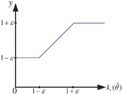
Figure 2 Crop function.
Looking further, the objective function of the clipping form () fundamentally depends on changes in the policy probability ratio (). When an action’s advantage estimate is positive, i.e., (), maximizing () drives the policy ration to increase, but this increase is capped by the upper bound () to prevent excessive policy updates. Conversely, when the action’s advantage estimate is negative, i.e., (), the optimization process drives to decrease, but its minimum value cannot fall below (). As shown in Figure 3, this “interval constraint” effectively prevents excessive policy updates, thereby enhancing the stability of the training process.
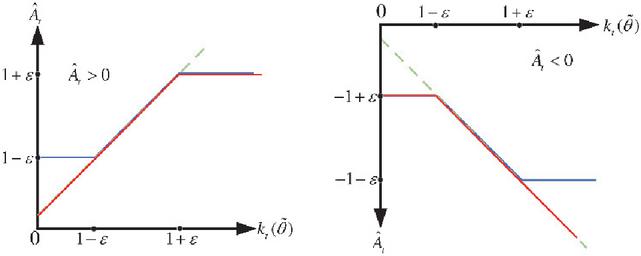
Figure 3 The PPO algorithm’s objective function following trimming.
As illustrated in Figure 3, the green curve represents the conventional (unclipped) surrogate objective, while the blue curve shows the clipped objective function used in PPO-clip. The red curve indicates the resulting objective after applying the minimum operation, which constrains the policy update within a safe range.
In PPO, the advantage function is employed to evaluate the relative value of actions, effectively removing the influence of the baseline state value . By doing so, the variance of the value estimation is reduced, leading to more accurate assessment of action quality. This refinement improves the stability and performance of the policy update, allowing the agent to learn more effectively while maintaining safe and incremental improvements in the expected return.
4 Case Studies
To validate the effectiveness and applicability of the proposed reinforcement learning and cooperative game-based source–grid–load–storage (SGLS) coordinated control method, this chapter conducts case studies using the IEEE 33-bus extended system and the IEEE 30-bus system as representative simulation platforms.
The evaluation focuses on multiple aspects:
1. Model Convergence: Assessing the learning stability and convergence speed of the RL-based coordination algorithm.
2. Operational Economy: Comparing system operating costs under different dispatch strategies.
3. System Stability: Evaluating voltage and frequency stability during coordinated control.
4. Coordinated Control Capability: Analyzing the interaction between energy storage and flexible loads in balancing generation and demand.
5. Robustness under Uncertainty: Testing the algorithm’s performance against variability in renewable generation and load demand.
All simulations are implemented in Python 3.9 using TensorFlow 2.10 and Keras, executed on a hardware platform comprising an AMD Ryzen 5 5600H CPU and an NVIDIA GTX 1650 GPU.
This setup enables comprehensive assessment of the proposed SGLS coordination strategy under realistic operational conditions and varying system uncertainties.
4.1 Construction of Simulation System and Dataset Generation
(1) IEEE 33-Bus Extended Distribution System
A simulation environment is established based on the IEEE 33-bus distribution network, with a nominal voltage of 12.66 kV. The original network topology is retained (Figure 4), while several extensions are implemented to represent a multi-source, multi-load system:
• Wind Power Integration: A 1 MW wind farm is connected at Bus 18.
• Photovoltaic Deployment: PV plants of 0.6 MW and 0.3 MW are installed at Buses 33 and 21, respectively.
• Energy Storage Systems: Three storage units are installed at Buses 7, 17, and 32, with maximum charge/discharge powers of 0.4 MW, 0.2 MW, and 0.2 MW, and capacities of 1.2 MWh, 0.6 MWh, and 0.6 MWh.
• Flexible Loads: Two types of flexible loads are modeled at each bus, consistent with the original load distribution: time-of-day adjustable loads and distributed controllable loads. The total active load is maintained at 2 MW.
Wind, PV, and load outputs are modeled with a constant power factor, while storage cost parameters, flexible load compensation, and control costs are assigned according to relevant literature.
(2) Dataset Generation
To capture stochastic behavior at different time scales, Monte Carlo simulations are conducted over 500 operational days. Forecast errors are added as normally distributed noise at 1-hour and 5-minute intervals, reflecting both slow-varying deviations and fast fluctuations in generation and load.
The resulting dataset is split into training and testing sets with an 8:2 ratio, providing the foundation for reinforcement learning-based optimization and evaluation of the coordinated source–grid–load–storage control strategy.
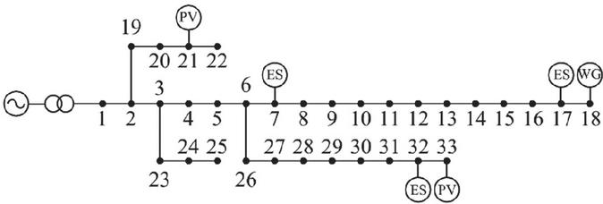
Figure 4 IEEE 33 example system.
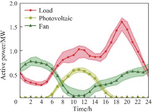
Figure 5 Uncertain range five days prior.
Figure 5 illustrates the forecast intervals for wind, solar, and load power over the day-ahead period, along with the corresponding typical actual power profiles for a representative day. Meanwhile, Figure 6 presents the minute-level intraday power fluctuations and highlights their amplification effects on tie-line flows, emphasizing the impact of high-frequency variability on network operation.
These visualizations provide insight into both the predictable trends and the short-term uncertainties inherent in renewable generation and load demand, forming a basis for evaluating the effectiveness of the proposed coordinated dispatch and real-time control strategies.
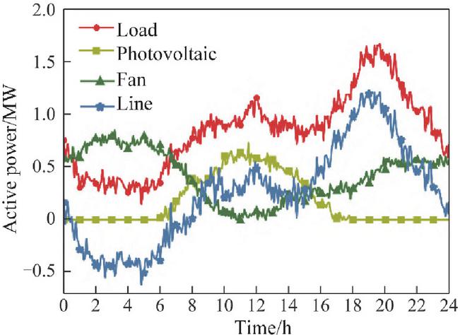
Figure 6 Variations in daily power.
(3) IEEE 30-Bus Transmission–Distribution Hybrid System
To further evaluate the generalization capability of the proposed coordinated control method in medium- and high-voltage transmission–distribution hybrid systems, a second case study is constructed based on the IEEE 30-bus system, as shown in Figure 7. The system configuration includes:
• Network Topology: 30 buses, 6 thermal generators, 42 transmission lines, and 20 load buses.
• Wind Integration: A 55 MW wind farm connected at Bus 28.
• Photovoltaic Integration: A 45 MW PV plant at Bus 14, yielding a renewable penetration of approximately 23%.
• Energy Storage Systems: Two storage units at Bus 5 and Bus 22, with capacities of 18 MWh/28 MW and 25 MWh/35 MW, respectively.
• Adjustable Loads: Controllable loads at Bus 6 and Bus 29 with a peak curtailment capability of 18 MW, and regulation costs referenced from literature.
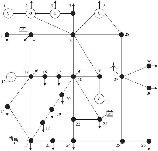
Figure 7 Configuration of the IEEE 30-bus transmission–distribution hybrid system with integrated renewable energy, energy storage, and controllable loads.
(2) Dataset and MDP Configuration
To simulate realistic operating conditions, actual wind and solar data from the Belgian grid are used, augmented with 5% stochastic variations to generate a multi-scenario dataset.
For the entire system, the MDP state space is defined with 34 dimensions, and the action space consists of 12 controllable variables, including generator outputs, storage charge/discharge powers, and adjustable load settings.
This setup enables assessment of the proposed reinforcement learning and cooperative game-based coordination strategy under diverse operating conditions, demonstrating its adaptability to larger and more complex hybrid networks [30].
4.2 Algorithm Convergence and Comparative Analysis
The performance of deep reinforcement learning algorithms is closely related to the choice of network architecture and hyperparameters. In this study, the detailed network structure and hyperparameters are summarized in Table 1.
For the simulation cases presented, in order to balance the quality of extracted features and dimensionality reduction, the day-ahead control feature extraction network employs a convolutional layer count of . This configuration provides sufficient representational power to capture the spatiotemporal patterns of renewable generation, load demand, and storage dynamics while maintaining computational efficiency. Unlike traditional MARL methods that treat agents as independent entities, this study integrates cooperative game theory to align agents’ incentives with overall system performance. The proposed method enhances stability, fairness and interpretability, which are often limited in conventional approaches.
Table 1 Network architecture and hyperparameter settings for the reinforcement learning-based coordinated dispatch algorithm
| Parameter | Value/Setting | Description |
| Network Type | CNN + Fully Connected | Convolutional layers for feature extraction, followed by dense layers |
| Number of Convolutional Layers | 6 | Number of convolutional layers in day-Ahead feature extraction network |
| Convolution Kernel Size | 3 3 | Kernel size for all convolutional layers |
| Number of Filters per Layer | 32, 64, 64, 128, 128, 256 | Number of feature maps in each convolutional layer |
| Activation Function | ReLU | Applied after each convolution and dense layer |
| Fully Connected Layers | 2 | Number of dense layers after convolutional feature extraction |
| Neurons per Fully Connected Layer | 256, 128 | Number of neurons in each dense layer |
| Learning Rate | 0.0003 | Initial learning rate for Adam optimizer |
| Discount Factor () | 0.99 | Discount factor for cumulative reward |
| Batch Size | 64 | Mini-batch size for network training |
| Training Episodes | 2000 | Total episodes for reinforcement learning |
| Replay Buffer Size | 50,000 | Experience replay buffer capacity |
| Clipping Parameter () | 0.2 | PPO-clip probability ratio clipping range |
The convergence of the proposed reinforcement learning-based coordination algorithm is evaluated across multiple simulation runs, and its performance is compared with benchmark methods to demonstrate the effectiveness, stability, and learning efficiency of the proposed SGLS (Source–Grid–Load–Storage) coordinated control strategy.
The training performance of the deep reinforcement learning algorithm is evaluated by monitoring the variation of the agent’s reward over time. During the simulations, several multi-objective weighting coefficients are used to balance different optimization goals: The ratio between the daily operating cost coefficient () and the tie-line power smoothing coefficient () governs the relative emphasis on economic efficiency versus network stability in day-ahead scheduling. The ratio between the storage day-ahead tracking coefficient () and the power fluctuation mitigation coefficient determines the priority between planned energy storage dispatch and intraday smoothing of power fluctuations. The ratio between the SOC correction coefficient () and the SOC deviation penalty coefficient () affects the agent’s tolerance for deviations in energy storage state-of-charge. Excessively large () may cause overly conservative storage re-dispatch.
The final selected multi-objective weight values are summarized in Table 2.
Table 2 Multi-objective weighting coefficients for day-ahead and intraday coordinated dispatch
| Coefficient | Value | Description |
| () | 0.5 | Day-ahead operating cost weight |
| () | 0.3 | Tie-line power smoothing weight |
| () | 0.4 | Storage day-ahead tracking weight |
| () | 0.2 | Intraday power fluctuation mitigation weight |
| () | 0.6 | SOC correction weight |
| () | 0.1 | SOC deviation penalty weight |
To mitigate stochastic effects, ten independent training runs are performed with different random seeds. Figures 8 and 9 illustrate the convergence of the day-ahead and intraday agents, respectively. The shaded regions indicate the range of reward fluctuations across ten runs, while the dark curves represent the average reward trajectory.
During training, the reward oscillates within a certain range before gradually converging toward a stable value. Moreover, MARL plays a crucial role in enhancing convergence by allowing agents (generation, grid, load, and storage) to collaboratively learn optimal strategies. This collaborative learning approach fosters fairness in decision-making, ensuring that all agents receive adequate incentives, thus preventing disparities in the benefits achieved by different entities. The stability of the system is also significantly improved, as agents are encouraged to maintain cooperation over time, reducing the likelihood of oscillations or performance degradation that may arise in non-cooperative settings. This indicates that, after the specified number of training episodes, both the day-ahead and intraday agents are able to effectively converge. The remaining fluctuations in the reward reflect the inherent uncertainty in the system states, which is expected in stochastic environments.
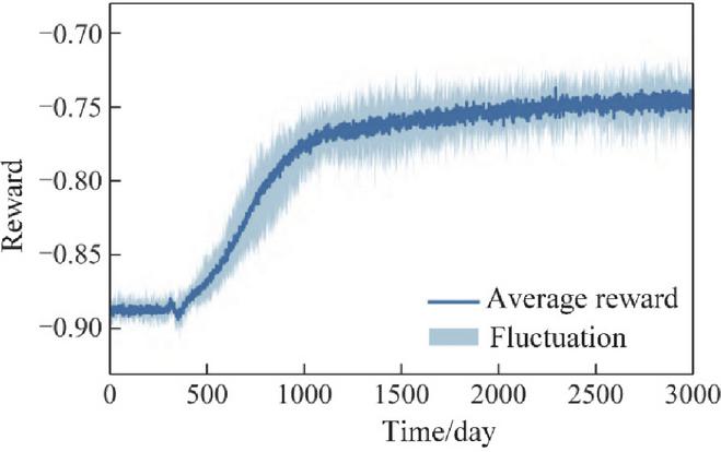
Figure 8 Convergence of the day-ahead agent: average reward and variation across ten training runs.
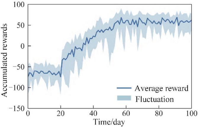
Figure 9 Convergence of the intraday agent: average reward and variation across ten training runs.
To evaluate the effectiveness of the proposed feature extraction network, its performance is compared with two alternative network structures: a fully connected (FC) network and an () convolutional network (CNN) [14]. The convergence results for these three network structures are illustrated in Figure 10.
When using the fully connected network, the network struggles to capture meaningful patterns due to the high redundancy in the distribution grid state matrix. This leads to poor fitting performance, causing the agent to learn data features inefficiently. The reward convergence curve exhibits noticeable oscillations, and the resulting optimization performance is suboptimal.
Using the () convolutional network improves feature extraction by capturing local spatial correlations in the state matrix. However, this network does not explicitly model the spatiotemporal relationships among variables across multiple stages. Consequently, while convergence and optimization performance are better than the FC network, the results still show considerable variability between independent experiments, indicating a degree of randomness in the optimization outcome.
In contrast, the proposed feature extraction network achieves rapid convergence to near-final reward values, with smaller variations across independent runs. This demonstrates both enhanced stability and superior optimization performance, confirming that the proposed network structure can effectively improve the convergence speed and overall effectiveness of the reinforcement learning-based coordinated dispatch algorithm.
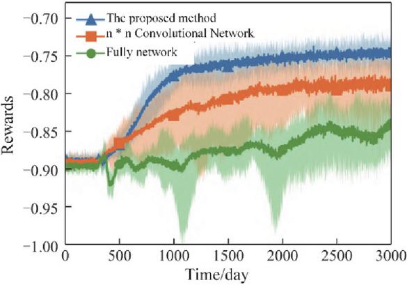
Figure 10 Comparison of convergence performance for different feature extraction networks: fully connected, convolutional, and proposed network.
To assess the effectiveness and superiority of the proposed method under uncertain operating conditions, the optimization results of the test dataset are compared across three approaches: the proposed deep reinforcement learning-based method, Method 1, and Method 3. Here, Method 3 does not account for source–load uncertainty and directly solves the day-ahead deterministic optimization model using a genetic algorithm, while Method 1 incorporates uncertainty through a scenario-based approach.
The distributions of the optimization objective values obtained by the three methods are presented in Figure 11.
From Figure 11, several observations can be made: Method 3 produces a highly irregular distribution of optimization values, with some values clustered near certain points but overall spread widely. This indicates that ignoring source–load uncertainty significantly degrades optimization performance in stochastic environments. Method 1 generates a more concentrated distribution by considering representative scenarios of source–load uncertainty. However, multiple peaks are still observed, reflecting potential mismatches between the reduced scenario set and the actual probability distribution of uncertainties. The proposed method achieves a distribution pattern similar to Method 1 but more concentrated around the optimal region, indicating that the reinforcement learning agent effectively learns the underlying uncertainty patterns from the dataset.
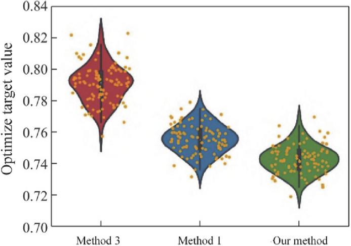
Figure 11 Comparison of optimization objective value distributions under uncertain source–load conditions for the proposed method, method 1 and method 3.
4.3 Analysis of Simulation Results
To verify the generalizability of the proposed multi-objective optimization approach, day-ahead scheduling is used as an example. The cumulative reward reflects the overall system performance by incorporating economic efficiency, stability, and flexibility, whereas SOC deviation measures the accuracy of energy storage management. Tie-line power MSE indicates the effectiveness of the system in smoothing power fluctuations, while operating costs provide insight into the economic feasibility of the scheduling strategy. These metrics collectively assess how well the system meets the objectives of cost reduction, power stability, and efficient energy storage management. By varying the weighting factors during training, a random day from the test set is selected to calculate the corresponding optimization objective values. The results before control and under different weighting factor settings are summarized in Table 3.
It can be observed that after day-ahead control, the total operational cost increases slightly. The major component remains the electricity procurement cost, while the proportion of energy storage control cost rises, reflecting the currently higher per-unit regulation cost of storage systems.
When the tie-line power smoothing weight is increased, the mean squared deviation of tie-line power decreases, indicating improved peak-shaving performance. However, the storage control cost rises accordingly, leading to a slight increase in total operational cost. The flexible load regulation cost shows no significant change, suggesting that flexible loads provide cost-effective peak-shaving under current cost parameters.
By appropriately adjusting network power flows throughout the day, the day-ahead control reduces network losses. For example, when and , the active power network loss cost decreases by 35.2%, and the tie-line power mean squared deviation decreases by 58.6%, demonstrating the effectiveness of multi-objective optimization.
Table 3 Day-ahead optimization results under different weighting factors
| Total | Electricity | Energy | Flexible | Tie-Line | Network | |
| Operational | Procurement | Storage | Load | Power | Loss | |
| Cost | Cost | Cost | Cost | MSE | Cost | |
| Scenario | (k$) | (k$) | (k$) | (k$) | (MW2) | (k$) |
| Before Control | 120.5 | 85.3 | 5.2 | 3.1 | 12.8 | 26.4 |
| 124.3 | 83.7 | 9.1 | 3.0 | 7.5 | 17.2 | |
| 126.1 | 82.5 | 11.3 | 3.1 | 5.3 | 16.1 | |
| 127.8 | 81.8 | 12.7 | 3.0 | 4.2 | 16.0 |
Figure 12 illustrates the tie-line power between the distribution network and the upstream grid before and after day-ahead control. It can be observed that during the 0–5 h period, the power exported from the distribution network to the upstream grid is significantly reduced. This is primarily because the energy storage system is charging at this time, absorbing a large portion of the wind generation output.
During the 15–21 h peak load period, the distribution network demand is effectively mitigated. Both energy storage and flexible loads work in coordination to reduce the peak power requirement. Within the controllable time windows of flexible loads, the agent redistributes part of the load originally scheduled between 15–19 h to the 9–14 h and 21–22 h intervals, achieving a peak-shaving and valley-filling effect.
Overall, the day-ahead control strategy smooths power fluctuations in the distribution network and alleviates the peak-shaving burden on the upstream grid. In practical operation, the weighting of different objectives can be adjusted based on the requirements of the distribution and upstream networks to achieve multi-objective optimization.
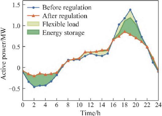
Figure 12 Day-ahead tie-line power profiles before and after coordinated control.
Figures 13 and 14 present the intraday regulation performance of three approaches: Method 4 (full smoothing), Method 5 (single-step optimization), and the proposed method. Figure 13 shows the tie-line power profiles before and after intraday control, while Figure 14 illustrates the energy storage day-ahead planned output, actual intraday output, planned SOC, and actual SOC for each method.
From Figure 14, it can be seen that during most periods, the proposed method and Method 5 generate energy storage power schedules similar to Method 4, indicating effective smoothing of power fluctuations. During periods of high variability, both the proposed method and Method 5 moderate the smoothing of tie-line power to prevent excessive deviations in storage SOC.
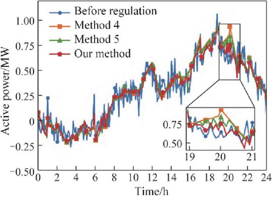
Figure 13 Intraday tie-line power profiles before and after control for method 4, method 5, and the proposed method.
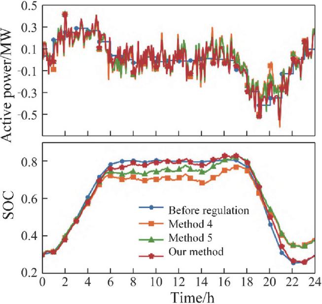
Figure 14 Energy storage day-ahead planned output, intraday actual output, planned SOC, and actual SOC for method 4, method 5, and the proposed method.
The key differences between the proposed method and the comparison approaches occur in the 6–8 h and 18–20 h periods. 6–8 h period: Tie-line power deviates from the day-ahead forecast. Methods 4 and 5 strictly track the scheduled power by aggressively adjusting storage output, resulting in significant SOC deviations. In contrast, the proposed method accounts for the impact of current control actions on subsequent periods, allowing for a partial relaxation of tie-line tracking. This reduces SOC deviations and preserves additional regulation capacity. 18–20 h period: Tie-line power again exhibits large deviations. Both the proposed method and Method 5 balance fluctuation suppression and SOC tracking, but Method 5 optimizes each time step independently and does not proactively correct SOC deviations, leading to residual discrepancies between initial and final SOC. The proposed method considers the full-period optimization effect, maintaining SOC deviations within a narrow range and significantly reducing the difference between initial and final SOC. During periods with rapid source–load fluctuations, storage power may frequently cross zero. This phenomenon can be managed by distributing control commands across multiple storage systems and units, which is not discussed in this study.
The intraday control performance of the three methods is summarized in Table 4. Before control: The energy storage system strictly follows the day-ahead schedule, resulting in zero SOC deviation. The tie-line power fluctuations fully reflect the source–load variability. Method 4 (full smoothing): Tie-line power fluctuations are completely suppressed, causing large deviations in storage SOC and a corresponding reduction in cumulative reward. Method 5 (single-step optimization): Optimizes tie-line power at each time step, balancing fluctuation suppression and SOC tracking, which improves the cumulative reward compared to Method 4. Proposed method: Considers both objectives and the impact of current actions on future periods, achieving a higher cumulative reward over the entire intraday control period.
Table 4 Intraday control performance metrics for different methods
| Tie-Line Power | Max SOC | Cumulative | |
| Method | MSE (MW2) | Deviation (%) | Reward |
| Before Control | 10.8 | 0 | 85.2 |
| Method 4 (Full Smoothing) | 2.1 | 15.4 | 72.5 |
| Method 5 (Single-Step) | 3.8 | 8.7 | 80.6 |
| Proposed Method | 3.5 | 4.2 | 88.1 |
To convert the system dispatch model into an MDP, the state space and action space must be defined. For the PPO algorithm: State space: Includes current time step (1 dimension), load forecasts (22 nodes), PV forecast (1 dimension), wind forecast (1 dimension), previous step outputs of thermal units (6 dimensions), actual PV output (1 dimension), actual wind output (1 dimension), curtailable load reductions (2 dimensions), and actual SOC of storage units (2 dimensions). The total state dimension is 36. Action space: Includes thermal unit outputs at time (6 dimensions), curtailable load adjustments (2 dimensions), and predicted SOC changes of storage units (2 dimensions), for a total action dimension of 10. The PPO algorithm parameters are set as follows: discount factor , clipping factor . The neural network is updated once every 120 scheduling cycles. The reward function parameters used in this case study are summarized in Table 5.
Table 5 Reward function parameters for IEEE 30-bus system
| Parameter | Value | Description |
| 0.45 | Day-ahead operating cost weight | |
| 0.35 | Tie-line power fluctuation penalty weight | |
| 0.25 | Storage SOC tracking weight | |
| 0.15 | Curtailable load regulation weight | |
| 0.50 | SOC correction coefficient | |
| 0.08 | SOC deviation penalty coefficient |
4.4 Case Study Results Analysis
In this study, three algorithms are applied for intraday optimization: PPO-clip, PPO with KL penalty (PPO-kl), and PPO-clip combined with KL penalty (PPO-clip-kl). The reward evolution curves during training are presented in Figure 15.
Each curve represents the reward obtained by the neural network before adjustment, evaluated over a randomly selected scheduling cycle. To account for stochastic effects, each environment is trained with 4 different random seeds, and the final curve is obtained by averaging the results across seeds. From Figure 15, it can be observed that all three algorithms show an overall increasing trend in reward values as training progresses, indicating effective learning of the intraday control policy. The PPO-clip-kl algorithm converges slightly faster and exhibits smoother reward curves compared to the other two, demonstrating improved stability and robustness. PPO-clip shows slightly larger fluctuations in the early training phase, while PPO-kl achieves moderate convergence speed but with occasional oscillations. These results indicate that combining clip constraints with KL penalty helps balance policy update stability and learning efficiency, making PPO-clip-kl more suitable for intraday optimization in complex, uncertain distribution systems.
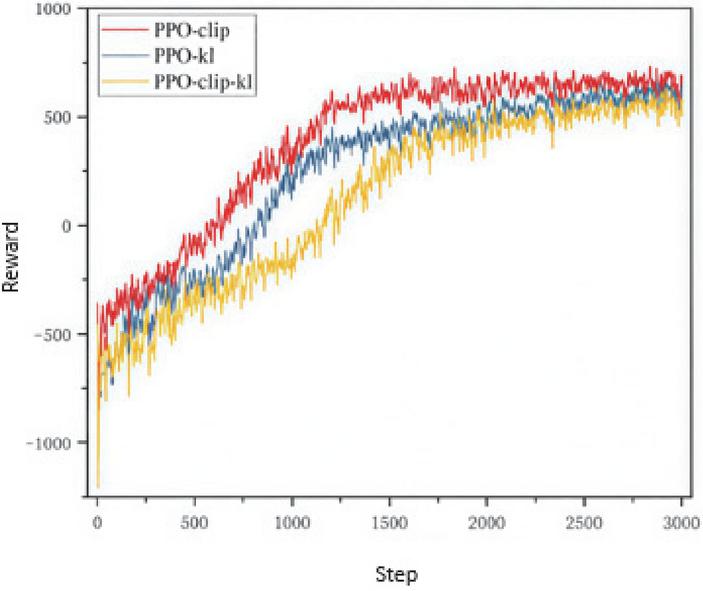
Figure 15 Training reward evolution for intraday optimization using PPO-clip, PPO-kl, and PPO-clip-kl algorithms.
Figure 15 presents the reward evolution curves of the three PPO variants used for intraday optimization. Overall, all algorithms demonstrate good convergence behavior.
During the initial training phase, the agent performs random exploration, and many actions violate the system’s operational constraints, particularly the power balance requirement, resulting in negative rewards. As training progresses, the policy network is updated continuously, reducing violations and gradually guiding the agent toward economically optimal scheduling.
In the later stages, minor fluctuations in the reward values occur due to variations in load and renewable generation across different scenarios, which affect the intraday optimization cost for each scheduling cycle. This variability is normal and expected in stochastic environments.
Since the reward function is designed based on system operational costs, it has an upper limit. After sufficient training cycles, the convergence values of the three algorithms are roughly similar. Among them, PPO-clip achieves the fastest convergence, as the clipping function constrains the update range of the advantage function, ensuring stable and efficient policy updates.
The PPO-clip-kl algorithm balances stability and learning speed but introduces higher computational complexity, resulting in slightly slower convergence. Each policy update requires calculating both the KL divergence penalty and the clipping adjustment, which increases computational overhead compared to algorithms using only one of these mechanisms.
This analysis indicates that PPO-clip provides a good trade-off between training efficiency and stability, making it suitable for rapid intraday optimization in uncertain distribution system scenarios.
After completing the offline training, the PPO-clip algorithm is applied to evaluate a representative scenario, as illustrated in Figure 16. This test assesses the algorithm’s ability to generate real-time intraday dispatch decisions under realistic load and renewable generation conditions, verifying the effectiveness of the learned policy in uncertain operational environments.
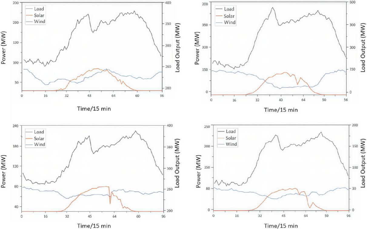
Figure 16 Representative scenario for intraday testing using the PPO-clip algorithm.
During the training process, to ensure adequate exploration of the environment and prevent the model from overfitting to the current experience replay, the action distribution is randomly sampled before mapping to the agent’s actual output range. Specifically, the Actor network computes the mean and variance of each controllable resource output, thermal unit generation, storage SOC, and curtailable load reduction, forming a normal distribution for each action. An action value is then sampled from this distribution, which promotes exploratory behavior and helps avoid local optima.
During testing, the agent selects the most probable action, corresponding to the mean of the distribution, which eliminates stochastic disturbances and ensures stable action execution. The test results on the validation dataset are shown in Figure 17, demonstrating the effectiveness and reliability of the trained PPO-clip policy in intraday dispatch under varying system conditions.
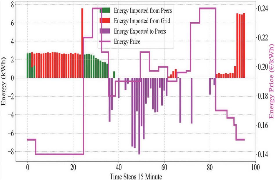
Figure 17 Test results of intraday dispatch using the PPO-clip algorithm.
After completing the offline training, a set of Actor network parameters is obtained. Using these parameters, online testing is conducted on four representative intraday scenarios. The dispatch plan for a typical day is illustrated in Figure 17.
By employing a rolling optimization approach, the agent determines the scheduling strategy for the entire day. The results demonstrate that the agent can adjust thermal unit outputs based on renewable generation forecasts, maximizing renewable energy utilization, accommodating output fluctuations, and ensuring system security.
From Figure 17, it can be observed that during 0:00–5:00, the load demand is generally lower than the minimum system supply, and the generation from renewables and thermal units exceeds demand. During this period, energy storage systems charge using surplus renewable generation. During peak load periods (19:00–22:00), the storage systems discharge, reducing peak load. By charging and discharging at different times, the storage system effectively shifts energy temporally, smoothing the load curve and achieving a peak shaving and valley filling effect. Additionally, during peak hours, curtailable loads actively participate in dispatch, alleviating pressure on the grid.
The economic cost comparison for testing scenario (a) using different algorithms is summarized in Table 6.
Table 6 Economic cost comparison for scenario (a) using different algorithms
| Algorithm | Day-Ahead Cost ($) | Intraday Cost ($) | Total Cost ($) |
| PPO-clip (Proposed) | 4,720 | 1,250 | 5,970 |
| PPO-kl | 4,750 | 1,280 | 6,030 |
| PPO-clip-kl | 4,730 | 1,260 | 5,990 |
| Method 4 (Full Smoothing) | 4,810 | 1,340 | 6,150 |
5 Conclusion
The proposed reinforcement learning and cooperative game-based method for coordinated regulation of generation, grid, load, and storage effectively enhances system economics, flexibility, and stability under high renewable energy penetration. By constructing a multi-dimensional state space and continuous action space MDP model, and employing the PPO algorithm for policy learning, the agent achieves dynamic optimal allocation of flexible resources in rolling daily scheduling. Simultaneously, the cooperative incentive mechanism incorporated into the reward function ensures coordinated benefits among all entities, preventing adverse behavior and enhancing overall system control efficiency. Extensive testing on IEEE 33-node and IEEE 30-node systems demonstrates superior performance compared to traditional optimization and other DRL strategies in convergence capability, operational costs, fluctuation suppression, and SOC management, showcasing strong generalization and robustness. Future work may further extend the multi-agent cooperative mechanism to practical power grid engineering scenarios, achieving higher-dimensional, multi-agent collaborative optimization.
Declaration
Funding Statement
Authors did not receive any funding.
Data Availability Statement
No datasets were generated or analyzed during the current study.
Conflict of Interest
There is no conflict of interests between the authors.
Declaration of Interests
The authors declare that they have no known competing financial interests or personal relationships that could have appeared to influence the work reported in this paper.
Ethics Approval
Not applicable.
Permission to Reproduce Material from Other Sources
Yes, you can reproduce.
Clinical Trial Registration
We have not harmed any human person with our research data collection, which was gathered from an already published article
Authors’ Contributions
All authors have made equal contributions to this article.
Author Disclosure Statement
The authors declare that they have no competing interests.
References
[1] Yang, H., Wei, X., Yang, Y., Li, Z., and Shen, S. (2024, September). Intelligent scheduling of source-grid-load-storage resources based on q-learning algorithm. In 2024 4th International Conference on Energy, Power and Electrical Engineering (EPEE) (pp. 1247–1251). IEEE.
[2] Ma, Y., Zhao, J., Yang, K., and Zeng, H. (2024, December). Research on Deep Learning-Based Collaborative Optimization Planning Strategy for Source-GridLoad-Storage Coordination. In 2024 4th International Conference on Intelligent Power and Systems (ICIPS) (pp. 633–636). IEEE.
[3] Zhou, D., Li, F., Zeng, P., Du, Z., and Jiao, K. (2024). Research on Key Technologies of “Source-Grid-Load-Storage” Collaborative Regulation and Interaction in the Park Based on Digital Twin Technology. In Mechatronics and Automation Technology (pp. 59–68). IOS Press.
[4] Zang, T., Wang, S., Wang, Z., Li, C., Liu, Y., Xiao, Y., and Zhou, B. (2024). Integrated planning and operation dispatching of source–grid–load–storage in a new power system: A coupled socio–cyber–physical perspective. Energies, 17(12), 3013.
[5] Cui, Z., Mo, C., Luo, Q., and Zhou, C. (2024). Integrated energy trading algorithm for source-grid-load-storage energy system based on distributed machine learning. Energy Informatics, 7(1), 149.
[6] Manas, M. (2018). Optimization of distributed generation-based hybrid renewable energy system for a DC micro-grid using particle swarm optimization. Distributed Generation & Alternative Energy Journal, 33(4), 7–25.
[7] Meydani, A., Shahinzadeh, H., Ramezani, A., Moazzami, M., Nafisi, H., and Askarian-Abyaneh, H. (2024, February). Comprehensive review of artificial intelligence applications in smart grid operations. In 2024 9th International Conference on Technology and Energy Management (ICTEM) (pp. 1–13). IEEE.
[8] Bai, F., and Zhang, K. (2025). The research progress on distributed generation and microgrid system stability: Progress, challenges, and frontier directions. Advances in Resources Research, 5(4), 2366–2408.
[9] Zhang, C., Roh, B. H., and Shan, G. (2024, June). Federated anomaly detection. In 2024 54th Annual IEEE/IFIP International Conference on Dependable Systems and Networks-Supplemental Volume (DSN-S) (pp. 148–149). IEEE.
[10] Li, Y., Zhou, T., and Jin, G. (2025). The research progress on multi-energy system integrated stability: Modeling methods, stability analysis, and coordinated control strategies. Advances in Resources Research, 5(4), 2409–2453.
[11] Kumar, P. M., Kamruzzaman, M. M., Alfurhood, B. S., Hossain, B., Nagarajan, H., and Sitaraman, S. R. (2024). Balanced performance merit on wind and solar energy contact with clean environment enrichment. IEEE Journal of the Electron Devices Society, 12, 808–823.
[12] Zhou, Y. (2024). Energy-Sharing Economy with Renewable Integration and Management in Communities – a State-of-the-Art Review. Advanced Energy and Sustainability Research, 5(12), 2400214.
[13] Ruiyi, C., Rui, G., Qisheng, L., Xingwang, J., Ling, S., Guanbao, Z., and Jia, H. (2025, April). Analysis of an IoT-Based Multi-Agent Relay Protection System and Cooperative Control Strategies. In 2025 10th Asia Conference on Power and Electrical Engineering (ACPEE) (pp. 1093–1097). IEEE.
[14] Li, Y., Li, Y., Song, Z., and Ma, Z. (2025). The research on resilient power system construction for high-proportion renewable energy: Responsiveness enhancement and intelligent development pathways. Advances in Resources Research, 5(3), 1381–1421.
[15] Yaoxin, W., Chun, Z., Lin, J., Houming, S., Qirui, W., and Zhuo, W. (2025, March). A Comprehensive Review on the Application of Artificial Intelligence in the Planning of the New-Type Power Systems. In 2025 7th Asia Energy and Electrical Engineering Symposium (AEEES) (pp. 1373–1382). IEEE.
[16] Miao, L., Zhou, N., Ma, J., Liu, H., Zhao, J., Wei, X., and Yin, J. (2025). Current Status, Challenges and Future Perspectives of Operation Optimization, Power Prediction and Virtual Synchronous Generator of Microgrids: A Comprehensive Review. Energies, 18(13), 3557.
[17] Deepak, K., Mandal, R. K., and Verma, V. (2023). Power Quality Improvement of a Hybrid Renewable Energy Sources Based Standalone System Using Neuro-Fuzzy Controllers. Distributed Generation & Alternative Energy Journal, 1815–1838.
[18] Gao, X., Zhang, J., Sun, H., Liang, Y., Wei, L., Yan, C., and Xie, Y. (2024). A review of voltage control studies on low voltage distribution networks containing high penetration distributed photovoltaics. Energies, 17(13), 3058.
[19] Mulevu, C. M., Okeyo, G. O., and Wafula, J. M. (2025). Data stream mining techniques for real-time monitoring and control of smart power grids in Kenya: challenges and opportunities. Discover Internet of Things, 5(1), 51.
[20] Wang, K., Huang, Y., Liu, Y., Huang, T., and Zang, S. (2025). A Review of Optimization Scheduling for Active Distribution Networks with High-Penetration Distributed Generation Access. Energies, 18(15), 4119.
[21] Zhu, L., Wu, X., Wang, Z., Li, Y., Song, L., and Yang, Y. (2025). A Study on the Environmental and Economic Benefits of Flexible Resources in Green Power Trading Markets Based on Cooperative Game Theory: A Case Study of China. Energies, 18(17), 4490.
[22] He, Y., Liu, T., Wang, Z., Ren, Q., and Chen, A. (2025). Adaptive and Collaborative Hierarchical Optimization Strategies for a Multi-Microgrid System Considering EV and Storage. World Electric Vehicle Journal, 16(7), 363.
[23] Gu, S., Qian, K., and Yang, Y. (2025). Optimization of Electric Vehicle Charging and Discharging Strategies Considering Battery Health State: A Safe Reinforcement Learning Approach. World Electric Vehicle Journal, 16(5), 286.
[24] Zhang, Z., Li, Y., Lai, D., Zhou, N., Zhan, Q., and Wang, W. (2025). Quantifying Weather’s Share in Dynamic Grid Emission Factors via SHAP: A Multi-Timescale Attribution Framework. Processes, 13(11), 3393.
[25] Wang, D., and Wu, S. (2025). Accurate Modeling of Carbon Emissions Under Urban Energy Consumption. Distributed Generation & Alternative Energy Journal, 1259–1280.
[26] Liu, C., Ye, C., Xu, J., Wang, Z., Wei, S., Yang, J., … and Liu, F. (2025, August). An Optimal Configuration Model For Photovoltaic And Energy Storage Access To The Distribution Network Considering Demand Response And EV Load. In 2025 3rd International Conference on Power, Grid and Energy Storage (pp. 283–288). IEEE.
[27] Liu, H., Yu, J., Wang, M., Zhou, M., and Wang, D. (2025). Source-load joint forecasting of office building electro-thermal integrated energy systems based on multi-task learning and dynamic optimal integration. International Journal of Green Energy, 1–19.
[28] Kulkarni, S. H., Jirage, B. J., and Anil, T. R. (2017). Alternative energy options for India – a multi-criteria decision analysis to rank energy alternatives using analytic hierarchy process and fuzzy logic with an emphasis to distributed generation. Distributed Generation & Alternative Energy Journal, 32(2), 29–55.
[29] Jiang, H., Tong, B., Yao, Z., and Zhao, Y. (2025). Hierarchical Distributed Low-Carbon Economic Dispatch Strategy for Regional Integrated Energy System Based on ADMM. Energies, 18(17), 4638.
[30] Shi, Z., Yan, L., Hu, Y., Wang, Y., Qin, W., Liang, Y., … and Zhang, Z. (2024). Optimization of operation strategy of multi-islanding microgrid based on double-layer objective. Energies, 17(18), 4614.
Biographies

Jinzhong Li received his Master’s degree from the University of Science and Technology of China in June 2015. He is currently a Faculty Member and serves as Professional Deputy Chief Engineer at the Electric Power Research Institute of State Grid Anhui Electric Power Co., Ltd., where he has been working since August 2015. His research interests focus on power system operation, dispatching technologies, and intelligent grid applications.

Yuguang Xie received his Ph.D. degree from Shanghai Jiao Tong University in June 2011. He is currently a Level 5 employee at the Electric Power Research Institute of State Grid Anhui Electric Power Co., Ltd., where he has been serving since August 2011. His main research interests include power system analysis, electricity markets, and advanced power grid control technologies.

Wei Ma obtained his Ph.D. degree from Beijing Jiaotong University in June 2021. He is currently the Person in Charge at the Electric Power Research Institute of State Grid Anhui Electric Power Co., Ltd., a position he has held since July 2021. His research interests include smart grid technologies, distributed energy systems, and data-driven power system optimization.

Kun Huang received his Bachelor’s degree from Nanjing University of Aeronautics and Astronautics in July 2015. He is currently the Person in Charge at Hefei Zhongke Brain Intelligence Technology Co., Ltd., where he has been working since July 2015. His research focuses on artificial intelligence applications, brain-inspired intelligence systems, and industrial intelligent technologies.
Distributed Generation & Alternative Energy Journal, Vol. 41_2, 387–432
doi: 10.13052/dgaej2156-3306.4126
© 2026 River Publishers