Research on Microgrid Power Dispatch Optimization Based on an Improved Parrot Optimization Algorithm in Cloud Environments
Yan Li
HeNan Technical College of Construction, Zhengzhou, HeNan, 450064, China
E-mail: hnly1981 @126.com
Received 05 December 2025; Accepted 11 January 2026
Abstract
To address the issues of high operational costs and load factors in microgrids under current renewable energy conditions, this study proposes a grid scheduling strategy based on a parrot optimization algorithm incorporating chaotic and adaptive weighting. First, a scheduling model based on power operation costs and load rates in cloud-based microgrids is constructed. Second, logistic chaos is employed during the initialization of the parameter optimization algorithm to increase population diversity, whereas an adaptive weight adjustment strategy balances global and local exploration capabilities. Finally, simulation experiments validate the algorithm’s performance. Compared with the ACO, PSO, and PO algorithms, it reduces costs and power load factors by 63.4%, 45.7%, 8.3%, and 6%, respectively, in scenarios with small numbers of users and by 37.4%, 34.4%, 23.6%, and 6%, respectively, in scenarios with large numbers of users. 23.6%, 9.51%, 9.51%, and 1.18%, respectively. This demonstrates its ability to effectively reduce operational costs and lower power load rates, indicating significant practical value.
Keywords: Cloud environment, microgrid, population initialization, adaptive weighting.
1 Introduction
In recent years, as humanity has placed greater emphasis on energy and deepened its understanding of the harmonious coexistence between humans and nature, enhancing resource utilization and reducing fossil fuel consumption have become focal points for the power industry. Microgrids, which utilize multiple distributed power sources as energy supply units, offer advantages such as environmental friendliness, flexibility, and ease of implementation. However, because these grids connect directly to users, their structure is more complex than traditional distribution networks. Consequently, improving the coordination between various power sources and loads while ensuring a reliable power supply to users and maximizing the utilization of clean energy presents a significant challenge in microgrid dispatch [1]. To achieve optimal microgrid dispatch outcomes, researchers have employed metaheuristic algorithms to reduce scheduling costs and time [2]. However, the inherent drawbacks of metaheuristic algorithms—rapid convergence and susceptibility to local optima—have somewhat diminished their effectiveness in microgrid scheduling [3]. Consequently, research has shifted toward employing improved traditional metaheuristic algorithms and newer metaheuristic approaches. Compared with enhanced traditional methods, newer metaheuristics demonstrate superior performance.
The Parrot Optimization Algorithm [4], proposed by Lian Junbo et al. in 2024, is a novel metaheuristic optimization algorithm. Inspired by the typical behaviors of domesticated parrots, its core simulates behavioral patterns such as foraging, perching, group communication, and fear responses to strangers, establishing an “exploration-exploitation” integrated optimization mechanism. As a tool for solving global optimization problems, its design effectively integrates the randomness and regularity of biological behaviors. This approach yields distinct advantages in initial solution space exploration, escaping local optima, and enhancing optimization accuracy. It has been applied to medical-related problems and offers novel solution strategies for engineering optimization and resource scheduling domains.
Building upon this, we apply the parrot optimization algorithm to microgrid task scheduling in cloud environments. First, we construct a scheduling model that is based on force-driven operational costs and power load factors. Second, we propose a Parrot behavior optimization for the PO algorithm, incorporating logistic chaos-inspired group initialization and adaptive weighting. Finally, we evaluate the algorithm’s performance through benchmark function tests, which achieve favorable results across scenarios with varying numbers of users and power consumption patterns.
2 Related Research
Scholars worldwide have achieved substantial progress in microgrid research. We organize this work into two areas: microgrid dispatch models and microgrid optimization strategies using metaheuristic algorithms.
(1) Microgrid Dispatch Models
Microgrid dispatch models aim to determine optimal operational plans for distributed power sources within a microgrid over a future time period, achieving objectives such as economic efficiency, reliability, or environmental benefits. Owing to their robust global search capabilities and advantages in handling nonlinear, nonconvex optimization problems, metaheuristic algorithms are widely applied to solve complex microgrid dispatch challenges. For example, Martinez-Rico et al. [5] proposed a multiobjective scheduling model for hybrid renewable energy systems, employing a particle swarm optimization algorithm to maximize profits while minimizing battery degradation. To address the more intricate coordination scheduling of multimicrogrid systems, Li et al. [6] introduced an enhanced marine predator algorithm to optimize the operational scheduling of interconnected microgrids, emphasizing intersystem coordination and energy exchange. Similarly, Dong et al. [7] focused on power interactions among multiple microgrids, optimizing operational scheduling strategies via an enhanced differential evolution algorithm to reduce overall operational costs. Additionally, researchers have actively explored the application of novel metaheuristic algorithms to microgrid economic dispatch. For example, Mazrae et al. [8] utilized the marine predator algorithm to optimize the economic dispatch of grid-connected microgrids, covering commercial building loads while minimizing operational costs. Yu et al. [9] proposed a hybrid scheduling strategy based on an improved marine predator optimizer to address complex scheduling problems in microgrids, enhancing the optimization efficiency and solution quality. With respect to power load considerations, Zhou et al. [10] introduced a microgrid scheduling model based on an improved walking optimizer algorithm, incorporating electric vehicles to improve system flexibility and economic efficiency by optimizing charging and discharging strategies. With respect to model fusion, Wen et al. [11] combined deep learning forecasting with genetic algorithm optimization to achieve optimal load scheduling for community microgrids, addressing renewable energy fluctuations. Ghorbal et al. [12] demonstrated the application potential of the Ninja metaheuristic optimization algorithm in microgrid economic dispatch to achieve dual environmental and economic objectives. Chen et al. [13] proposed a scheduling optimization model for cost reduction in the intelligent era. Pan et al. [14] introduced a distribution network scheduling strategy to enhance load-generation forecasting for new energy sources.
(2) Microgrid Optimization Strategies
Microgrid optimization strategies extend beyond short-term scheduling to encompass long-term capacity allocation, control parameter optimization, and protection coordination. These strategies form the foundation for ensuring the long-term stable and economical operation of microgrids. Metaheuristic algorithms play a pivotal role in solving these high-dimensional, multiconstraint complex optimization problems. With respect to capacity allocation, researchers have focused on the use of metaheuristics to determine the optimal component size that minimizes costs while maximizing reliability. Diab et al. [15] employed modern metaheuristic algorithms for capacity optimization in standalone microgrids, aiming to minimize total lifecycle costs and enhance power supply reliability. Bouaouda et al. [16] proposed an optimization framework for capacity allocation in hybrid photovoltaic-wind systems with hydrogen storage and employed metaheuristic algorithms while accounting for component lifespan and system reliability. Castellanos-Buitrago et al. [17] extended the optimization scope to multiple years, utilizing metaheuristic algorithms to address multiyear capacity optimization in microgrids, thereby enhancing power supply reliability and efficiency. Islam et al. [18] employed the marine predator algorithm to optimize robust composite controller parameters for DC–AC microgrids, enhancing power sharing and real-time voltage stability. Regarding protection, Abdi et al. [19] utilized a novel metaheuristic algorithm to optimize the setting parameters of directional overcurrent relays in microgrids, achieving fast and reliable fault protection coordination. Xiong et al. [20] proposed a collaborative control technology for digital power grid construction in a cloud computing environment.
The above research findings demonstrate the irreplaceable core value of metaheuristic algorithms in microgrid-related studies. Microgrid systems encompass distributed generation, energy storage devices, and diverse loads, presenting core challenges such as operational optimization and capacity allocation with complex characteristics, including multiobjective, multiconstraint, nonlinear, and high-dimensional features. Traditional mathematical programming methods are prone to local optima and exhibit low solution efficiency. Leveraging its strengths in robust global search capabilities and broad adaptability, metaheuristic algorithms efficiently handle dynamic constraints such as renewable energy output variability and load fluctuations. They precisely identify Pareto optimal solutions that balance economic efficiency, environmental sustainability, and reliability, providing intelligent technical support for microgrid planning, real-time dispatch, and operational optimization. These algorithms serve as critical tools for advancing the large-scale deployment of microgrids and driving the low-carbon transformation of energy systems.
3 Microgrid Dispatch Optimization Model
We developed a model centered on the collaborative optimization of “multiperiod loads and multiple power supply units,” focusing on the joint dispatch of photovoltaic power, wind power, energy storage, and grid-purchased electricity. This approach achieves a dual-objective balance of “minimum operating costs” and “maximum power supply reliability” while meeting load electricity demands and adhering to physical equipment constraints. Let the set of power supply units be denoted as , specifically , representing the four power units: photovoltaic, wind power, energy storage, and grid-purchased electricity. The parameters of each power source are denoted as , where represents the maximum output of power supply unit , denotes the unit operating cost of the power supply unit, indicates the minimum output of the power source, and signifies the corresponding efficiency of the power supply unit. Let denote 24 consumption periods, with the load parameter for each period. Here, represents the power demand for period , and denotes the duration of period .
3.1 Constraint Setting
To ensure the physical feasibility of this model’s implementation, it must satisfy two types of constraints. Specifically:
(1) Power Unit Output Constraint
This constraint ensures that for any time period , the actual power supply allocated to power unit satisfies . Here, represents the minimum effective power supply of the power unit, and represents the maximum effective power supply of the power unit.
(2) Load–supply logic Constraint
For any time period , when the actual power supply satisfies all demand, the power shortage is 0. Otherwise, , and the power shortage is .
3.2 Objective Function Construction
This model employs a “dual-objective weighted normalization” design, constructing the function primarily around two key objectives: reducing operating costs and lowering the load power shortage rate, ultimately yielding a comprehensive optimal solution.
(1) Total operating cost
The sum of the power supply costs across all the time periods is mathematically expressed as follows:
| (1) |
where denotes the power supply units allocated to time period .
(2) Load power shortage rate
This ratio of total power shortage to total power demand, which is expressed mathematically as:
| (2) |
where represents the total power shortage during a day’s time period, denotes the total power demand for a day, and is the power shortage rate.
(3) Comprehensive Fitness Function
On the basis of the two factors of cost and time, this model primarily pursues dual core objectives: “minimizing the total operating cost” and “minimizing the load power shortage rate.” Since the total operating cost and total power shortage rate are optimization targets with different dimensions, normalization processing and weight allocation are required to effectively integrate the dual objectives, forming the following expression:
| (3) |
where and represent the weights for operating costs and the load outage rate, respectively, and where and denote the preset maximum cost and maximum outage rate, respectively.
4 Parrot Optimization Algorithm
The Parrot Optimization Algorithm primarily exhibits four distinct behavioral characteristics: foraging behavior, resting behavior, communication behavior, and fear of strangers. These parrot behaviors form the core framework of the algorithm. Each behavior is described below.
(1) Population Initialization
The initial population size of the entire parrot algorithm is set to , the maximum iteration count is set to , and the search space constraints with lower bound and upper bound . Therefore, the individual initialization expression for this algorithm is as follows:
| (4) |
In the formula, represents a random number within the range [0,1], and denotes the initial position of the th parrot.
(2) Foraging Behavior
Parrots estimate the location of target food by observing either the food’s position or their owner’s position and then fly toward the food. The expression formula for parrot movement is as follows:
| (5) |
In the equation, denotes the position of the th individual in the th iteration, and denotes the position of the th individual in the th iteration. represents the average position of all individuals in the current population, and denotes the Levy distribution used to describe the parrot flight patterns. denotes the optimal position within the current population. denotes movement relative to the optimal population position, whereas represents the entire population’s position to further determine the food direction. Additionally, the average position of the current population is denoted by , expressed as follows:
| (6) |
The Levy distribution can be obtained according to the rules in the following formula, where is set to 1.5.
| (7) |
(3) Perching Behavior
Parrots are highly social creatures, and their perching behavior primarily involves suddenly appearing near optimal locations within the flock, thereby introducing randomness into the search process. This behavior manifests as follows:
| (8) |
In the formula, denotes a vector of dimension filled with ones. represents flying toward the current population’s optimal solution, whereas denotes randomly stopping at the position of the population’s optimal solution individual.
(4) Communication Behavior
Parrots are inherently social creatures, exhibiting behaviors that involve both approaching and avoiding other groups. In the algorithm, both behaviors are assumed to occur with equal probability, with the current population’s average position representing the flock’s center. This behavior is expressed as follows:
| (9) |
In the formula, the value of the random number is set to simulate the absence of communication between individuals. When the random number is less than or equal to 0.5, it represents the process of an individual joining the parrot group for communication; otherwise, it represents the process of an individual immediately flying away after communication.
(5) Fear-Based Behavior
In general, parrots and other birds exhibit natural fear toward strangers, and parrots are no exception. Consequently, they will distance themselves from unfamiliar individuals and seek protection from their owners. This behavior manifests as follows:
| (10) |
In the equation, represents the process of redirecting toward the owner, whereas represents the process of moving away from strangers.
5 Microgrid Dispatch via an Improved Parrot Optimization Algorithm
5.1 Improved Parrot Optimization Algorithm-LAPO
Like most metaheuristic algorithms, the Parrot algorithm suffers from slow convergence and susceptibility to local optima, particularly when handling high-dimensional problems where its global search capability is weak. To enhance algorithmic performance, we employ logistic chaos for population initialization to increase solution diversity while using adaptive weights for algorithmic optimization to balance global and local equilibrium.
(1) Population Initialization Based on Logistic Chaos Mapping
In metaheuristic algorithms, the quality of population initialization directly impacts the solution accuracy and convergence speed. While the current Parrot algorithm employs a basic population initialization method, this approach still leads to insufficient population diversity, potentially causing premature convergence or becoming stuck in local optima. The literature [21, 22] demonstrates that employing population initialization based on logistic chaotic mappings in metaheuristic algorithms generates initial individuals with more uniform distributions and broader coverage across the solution space. Accordingly, this paper adopts logistic chaotic mappings for population initialization, expressed as follows:
| (11) | |
| (14) |
In Equation (11), denotes the mapping function, and denotes the parameter.
(2) Adaptive weight optimization
Traditional parrot algorithms employ fixed or simple linearly adjusted weighting strategies for their four behaviors, making it difficult to dynamically balance global exploration and local exploitation capabilities. Previous studies [23, 24] have demonstrated that adaptive weights can significantly enhance the search trajectory of metaheuristic algorithms, prevent premature convergence, and lead to faster convergence speeds and higher solution accuracy in high-dimensional complex problems. On this basis, this paper introduces a nonlinear decreasing adaptive weighting scheme that dynamically adjusts the movement step size and direction of individuals. This enhances exploration diversity in the early stages and accelerates convergence stability in the later stages. The adaptive weighting expression is as follows:
| (15) |
In the formula, represents the maximum iteration count, denotes the current iteration count, and indicates the maximum value of the weight. From the equation, it is evident that during the initial iterations, a larger value (approaching the maximum) endows the algorithm with strong global exploration capabilities, aiding in escaping local optima and extensively searching the solution space. As the number of iterations increases, gradually decreases, shifting the algorithm’s search behavior toward local refinement optimization and thereby enhancing the convergence accuracy in later stages. This adaptive adjustment better balances global and local search, prevents premature convergence or excessive random exploration, and improves the algorithm’s overall optimization performance. Consequently, foraging, resting, communication, and fear behaviors are defined as follows:
| (16) | ||
| (17) | ||
| (20) | ||
| (22) |
5.2 Algorithm Complexity
The time complexity of the LAPO algorithm is primarily influenced by the number of objective function evaluations and the population size. Its main loop iterates times, with each iteration updating individuals and calculating their fitness. Each individual update involves random number generation, Levy flight calculations, and four strategy selections. The strategy operations include fixed-number operations on dimension , resulting in a total time complexity of . Regarding space complexity, the algorithm requires storing the population position matrix , the fitness array , and intermediate variables during iteration. Additionally, chaotic initialization occupies units of space, resulting in a total space complexity of .
5.3 Microgrid Dispatch Process Based on the LAPO
Step 1: Initialize the core parameters of the LAPO algorithm, set the population size and maximum iteration count, and define the microgrid core parameters.
Step 2: Develop the individual encoding scheme for the LAPO algorithm, mapping each parrot individual to a set of microgrid scheduling schemes. The individual dimension equals the total number of scheduling periods, with each dimension’s value representing the power allocation ratio of PV, wind, storage, and grid power for each period.
Step 3: Define the fitness function using the microgrid scheduling objective function as the LAPO fitness metric.
Step 4: Initialize the LAPO algorithm population via logistic chaotic mapping to ensure that the initial scheduling schemes cover a reasonable range of power allocations;
Step 5: Establish adaptive weights to optimize the parrot algorithm’s foraging, resting, social interaction, and fear behaviors, enhancing the algorithm’s adaptability to dynamic scenarios;
Step 6: After each iteration, update the fitness values of the individuals. Real-time load fluctuations are incorporated to adjust the fitness calculations. If an individual’s current fitness surpasses its historical best value, its optimal solution is updated. Simultaneously, compared with the population’s global optimal solution, if the individual’s fitness exceeds the global optimum, update the global optimal solution.
Step 7: Determine if the algorithm meets the termination conditions. If not met, return to Step 6 to continue iterating; if met, terminate the search.
Step 8: Output the globally optimal individual identified by the LAPO algorithm. The corresponding power allocation plan for each time period constitutes the optimal scheduling strategy.
6 Simulation Experiments
To better demonstrate the effectiveness of the proposed algorithm in microgrid scheduling, we select the following hardware configuration: a Core i5 CPU, 16 GB DDR4 memory, and a 1 TB hard drive. The software environment comprises MATLAB 2024a and the Windows 10 operating system. The experiments comprise two parts: one verifies the improved parrot optimization algorithm, while the other evaluates the scheduling performance of the proposed algorithm in cloud-based microgrids. For comparison, we selected ant colony optimization (ACO), particle swarm optimization (PSO), the whale optimization algorithm (WOA), and particle swarm evolution (PSE) as benchmark algorithms.
6.1 Algorithm Performance Comparison
To better demonstrate the performance of the LAPO algorithm, we select Sphere, Schwefel1.2, Schwefel2.2.1, Step, Ackley, and Griewank as the primary test functions. These functions cover multiple typical optimization scenarios, comprehensively evaluating the algorithms’ capabilities in global search, local optimization, disturbance resistance, and handling problems with varying complexity. This ensures objective and thorough performance assessment. Additionally, we select the maximum value, minimum value, average value, and variance as evaluation metrics. These four metrics provide a comprehensive assessment of algorithm performance: extremes reflect optimization limits, averages indicate overall capability, variance characterizes result stability, and combined evaluation offers greater scientific rigor. The expressions for the six benchmark functions are shown in Table 1. The population size for all five algorithms was set to 30, with 100 iterations. The key algorithm parameters are detailed in Table 2. Table 3 presents the comparative results across the four metrics for the six benchmark functions. Figures 1–6 display the fitness function comparisons for the five algorithms on the six benchmark functions at a dimension of 30.
Table 1 Benchmark functions
| Function Name | Function | Range |
| Sphere | ||
| Schwefel1.2 | ||
| Schwefel2.21 | ||
| Step | ||
| Ackley | ||
| Griewank |
Table 2 Main parameters of the five algorithms
| Algorithm | Parameter Name | Value |
| ACO | Pheromone | 0.1 |
| Disturbance Factor | 0.95 | |
| PSO | Inertia Weight | 0.9 |
| Individual Learning Factor | 2 | |
| Social Learning Factor | 2 | |
| WOA | Control Parameter | 2 |
| Fixed Probability | 0.5 | |
| PO | 0.5 | |
| Random number | 0.5 | |
| LAPO | 3.9 | |
| Maximum Weight | 0.9 |
Table 3 Comparison of the four indicators of the five algorithms under different functions
| Function | Algorithm | Dim | Maxvalue | Minvalue | Average value | Sdvalue |
| Sphere | ACO | 5 | 4.5661e-15 | 4.4829e-18 | 3.6795e-16 | 8.7863e-16 |
| 30 | 3.0231e+02 | 3.0142e+01 | 9.3416e+01 | 6.3688e+01 | ||
| PSO | 5 | 3.3630e-02 | 2.2637e-04 | 6.9286e-03 | 8.4933e-03 | |
| 30 | 1.6537e+04 | 3.6672e+03 | 1.0396e+04 | 3.8654e+03 | ||
| WOA | 5 | 2.6618e-13 | 1.7400e-19 | 1.1499e-14 | 4.9510e-14 | |
| 30 | 2.5971e-11 | 3.5038e-15 | 4.5582e-12 | 6.9099e-12 | ||
| PO | 5 | 9.7374e-08 | 9.7548e-21 | 5.5927e-09 | 1.9346e-08 | |
| 30 | 1.1599e-04 | 0.0000e+00 | 6.2594e-06 | 2.2674e-05 | ||
| LAPO | 5 | 2.2868e-09 | 0.0000e+00 | 2.2721e-10 | 5.3045e-10 | |
| 30 | 5.5648e-06 | 0.0000e+00 | 1.9376e-07 | 1.0151e-06 | ||
| Schwefel1.2 | ACO | 5 | 3.7647e-07 | 4.2587e-10 | 2.8630e-08 | 6.9816e-08 |
| 30 | 4.6764e+04 | 5.4021e+03 | 2.7948e+04 | 8.1502e+03 | ||
| PSO | 5 | 1.8212e+00 | 5.5955e-02 | 3.5242e-01 | 3.9658e-01 | |
| 30 | 7.1536e+04 | 3.3258e+04 | 5.4848e+04 | 9.0601e+03 | ||
| WOA | 5 | 3.4314e+02 | 3.2851e-01 | 8.9493e+01 | 9.8059e+01 | |
| 30 | 1.6999e+05 | 5.2715e+04 | 9.3465e+04 | 3.4219e+04 | ||
| PO | 5 | 8.2960e-06 | 3.0672e-16 | 7.3128e-07 | 2.0801e-06 | |
| 30 | 5.2753e-02 | 0.0000e+00 | 1.8518e-03 | 9.6225e-03 | ||
| LAPO | 5 | 1.8308e-09 | 0.0000e+00 | 1.4010e-10 | 4.1354e-10 | |
| 30 | 4.1265e-07 | 0.0000e+00 | 3.4235e-08 | 8.5260e-08 | ||
| Schwefel2.21 | ACO | 5 | 5.7663e-07 | 3.1934e-08 | 1.5022e-07 | 1.4335e-07 |
| 30 | 9.1932e+01 | 1.9377e+01 | 7.1513e+01 | 2.0621e+01 | ||
| PSO | 5 | 1.9525e-01 | 2.1475e-02 | 9.9597e-02 | 5.3766e-02 | |
| 30 | 8.4419e+01 | 5.6214e+01 | 7.3096e+01 | 7.0270e+00 | ||
| WOA | 5 | 1.6806e+01 | 1.2949e-02 | 2.4429e+00 | 3.9629e+00 | |
| 30 | 9.1123e+01 | 5.9414e+00 | 6.5377e+01 | 1.8265e+01 | ||
| PO | 5 | 9.6412e-04 | 0.0000e+00 | 1.0958e-04 | 2.4223e-04 | |
| 30 | 1.0417e-02 | 0.0000e+00 | 5.3219e-04 | 1.8975e-03 | ||
| LAPO | 5 | 6.0339e-05 | 0.0000e+00 | 4.7178e-06 | 1.2002e-05 | |
| 30 | 6.4018e-04 | 0.0000e+00 | 4.9988e-05 | 1.3622e-04 | ||
| Step | ACO | 5 | 1.0876e-15 | 5.8761e-18 | 1.7662e-16 | 2.6930e-16 |
| 30 | 3.4603e+02 | 1.8644e+01 | 1.2227e+02 | 9.1094e+01 | ||
| PSO | 5 | 2.5241e-02 | 1.0854e-04 | 3.7967e-03 | 5.2264e-03 | |
| 30 | 2.2405e+04 | 2.0145e+03 | 1.0313e+04 | 5.8652e+03 | ||
| WOA | 5 | 2.2970e-01 | 7.1404e-05 | 1.9487e-02 | 4.2560e-02 | |
| 30 | 3.8356e+00 | 1.3845e+00 | 2.1589e+00 | 6.0180e-01 | ||
| PO | 5 | 2.4713e-02 | 9.6495e-05 | 4.2882e-03 | 5.7306e-03 | |
| 30 | 2.4937e+00 | 2.8444e-02 | 7.1075e-01 | 5.9079e-01 | ||
| LAPO | 5 | 6.3150e-03 | 4.8940e-05 | 1.6115e-03 | 1.7969e-03 | |
| 30 | 1.6749e+00 | 8.5924e-03 | 3.1169e-01 | 3.9636e-01 | ||
| Ackley | ACO | 5 | 3.6320e-08 | 1.1968e-09 | 7.4533e-09 | 7.4242e-09 |
| 30 | 1.5569e+01 | 3.1252e+00 | 5.0342e+00 | 2.2012e+00 | ||
| PSO | 5 | 1.9594e-01 | 9.9917e-03 | 4.9347e-02 | 4.1625e-02 | |
| 30 | 2.0463e+01 | 1.2057e+01 | 1.8357e+01 | 2.1677e+00 | ||
| WOA | 5 | 1.2829e-05 | 4.1587e-10 | 5.0176e-07 | 2.3430e-06 | |
| 30 | 2.7930e-06 | 7.5539e-09 | 4.6845e-07 | 6.1804e-07 | ||
| PO | 5 | 2.1284e-04 | 3.4253e-12 | 3.8234e-05 | 5.0071e-05 | |
| 30 | 2.2400e-02 | 4.4409e-16 | 1.5848e-03 | 4.3566e-03 | ||
| LAPO | 5 | 1.3473e-05 | 4.4409e-16 | 1.6700e-06 | 2.8581e-06 | |
| 30 | 2.0365e-04 | 4.4409e-16 | 3.5593e-05 | 5.4745e-05 | ||
| Griewank | ACO | 5 | 3.6792e-01 | 8.5729e-02 | 2.3761e-01 | 7.1520e-02 |
| 30 | 4.0171e+00 | 1.1801e+00 | 1.8683e+00 | 5.5724e-01 | ||
| PSO | 5 | 5.2676e-01 | 1.0789e-01 | 2.6868e-01 | 1.0151e-01 | |
| 30 | 1.8922e+02 | 2.0600e+01 | 7.4055e+01 | 3.7100e+01 | ||
| WOA | 5 | 7.5326e-01 | 1.1102e-16 | 2.2293e-01 | 2.2310e-01 | |
| 30 | 8.2867e-01 | 4.7851e-14 | 2.7622e-02 | 1.5129e-01 | ||
| PO | 5 | 1.5451e-05 | 0.0000e+00 | 6.5442e-07 | 2.8726e-06 | |
| 30 | 5.3044e-06 | 0.0000e+00 | 2.5233e-07 | 1.0142e-06 | ||
| LAPO | 5 | 1.5323e-01 | 0.0000e+00 | 1.0230e-02 | 3.2197e-02 | |
| 30 | 1.1605e-07 | 0.0000e+00 | 5.3626e-09 | 2.1426e-08 |
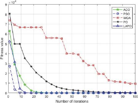
Figure 1 Sphere functions.
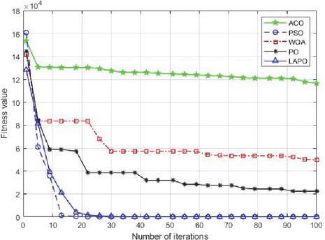
Figure 2 Schwefel1.2 function.
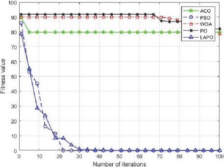
Figure 3 Schwefel2.21 functions.
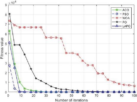
Figure 4 Step functions.
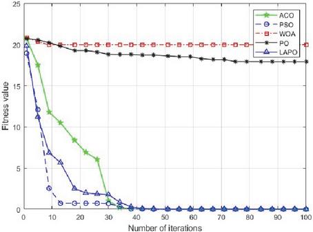
Figure 5 Ackley function.
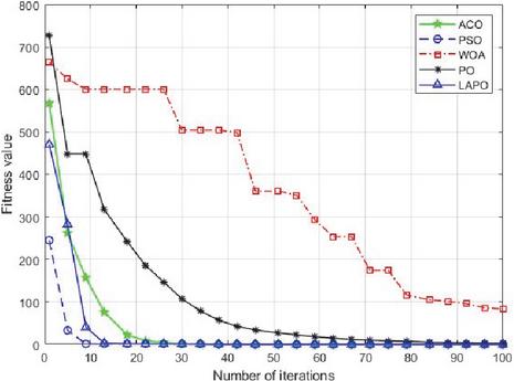
Figure 6 Griewank functions.
Table 3 presents the comparison results of the four indicators for the five algorithms under 5-dimensional and 30-dimensional conditions. The detailed analysis is as follows:
On the basis of the test results of the Sphere function, at a dimension of 5, the LAPO algorithm significantly outperforms the average values of ACO, PSO, WOA, and PO, with a minimum value of 0.0000e+00, an average value of 2.2721e–10, and a standard deviation of 5.3045e–10, demonstrating exceptional global optimal solution search capability. When the dimension reaches 30, most algorithms experience a significant decline in performance, whereas LAPO maintains a maximum value of 5.5648e-06, an average value of 1.9376e-07, and a minimum value of 0.
On the basis of the Schwefel 2.12 function test results, at a dimension of 5, LAPO achieves a minimum value of 0.0000e+00, an average of 1.4010e–10, and a standard deviation of 4.1354e–10, comprehensively outperforming the ACO and PSO averages. Even when the WOA reached a maximum of 3.4314e+02 and the PO averaged 7.3128e-07, LAPO maintained exceptional convergence accuracy. At 30 dimensions, LAPO achieved an average of 3.4235e-08 and a minimum of 0.
For the Schwefel 2.21 function, at dimension 5, LAPO achieves a minimum of 0, an average of 4.7178e-06, and a standard deviation of 1.2002e-05, outperforming all four comparison algorithms while demonstrating the best convergence precision and stability. At dimension 30, the mean values of ACO, PSO, and WOA all remained above 5e+01, whereas LAPO achieved a maximum of only 6.4018e-04, a mean of 4.9988e-05, and a minimum of 0.
On the basis of the step function test results, at dimension 5, LAPO outperforms the PSO, WOA, and PO averages, with a maximum of 6.3150e-03, an average of 1.6115e-03, and a standard deviation of 1.7969e-03. Only ACO approached the minimum value of LAPO, but LAPO exhibited lower overall volatility. At dimension 30, the ACO and PSO average values increased to 1.2227e+02 and 1.0313e+04, respectively, whereas the LAPO maintained a maximum of 1.6749e+00 and an average of 3.1169e-01, which were significantly lower than the averages of the WOA and PO.
On the basis of the Ackley function test results, at 5 dimensions, LAPO outperforms the average of the four algorithms, with a minimum value of 4.4409e-16, an average of 1.6700e-06, and a standard deviation of 2.8581e-06. At dimension 30, ACO and PSO achieve means of 5.0342e+00 and 1.8357e+01, respectively, but still fall short of the optimal solution. LAPO maintained a minimum of 4.4409e-16, with a mean of only 3.5593e-05 and a standard deviation of 5.4745e-05.
For the Griewank function test, at dimension 5, ACO and PSO had average values of 2.3761e-01 and 2.6868e-01, respectively, which were significantly higher than the LAPO values of 1.0230e-02. Although the WOA achieves a minimum value close to 0, its standard deviation of 2.2310e-01 indicates significantly lower stability than that of LAPO. While PO demonstrated higher accuracy, LAPO presented a clear advantage in convergence. At dimension 30, the ACO and PSO performances deteriorate significantly. Although the WOA achieved an average of 2.7622e-02, the LAPO recorded a maximum of only 1.1605e-07, an average of 5.3626e-09, and a minimum of 0.
On the basis of the results from the six benchmark functions above, the LAPO algorithm demonstrates excellent performance in both global search and local optimization. It exhibits particular stability under complex single-peak and high-dimensional multipeak conditions, showing outstanding capabilities.
Figures 1–6 present the fitness value analysis of the five algorithms across the six test functions. The convergence curves in Figure 1 show that ACO, PSO, and LAPO rapidly reduce fitness to near zero within the first 10 iterations, demonstrating significantly faster convergence than the WOA and PO. However, LAPO results in a smoother and more stable curve with no significant fluctuations. Its initial descent slope is steeper, retaining the rapid convergence characteristics of ACO and PSO while avoiding fluctuations in the WOA and the delayed acceleration of PO. This makes it superior in terms of speed, accuracy, and stability. As shown in Figure 2’s convergence curve, the LAPO algorithm rapidly reduces the fitness value from 1.6 104 to nearly 2 within the first 10 iterations, achieving convergence speeds far surpassing those of ACO, PSO, the WOA, and PO. Simultaneously, the curve of LAPO remains smooth and fluctuation-free throughout, making it the most balanced solution among these five algorithms. Figure 3’s convergence curve reveals that the LAPO algorithm rapidly reduces the fitness value from 100 to near 0 within the first 20 iterations, achieving convergence speeds far exceeding those of the comparison algorithms. This demonstrates LAPO’s superior comprehensive performance in terms of convergence speed, optimization accuracy, and stability. In the convergence curve of Figure 4, the LAPO algorithm rapidly reduces the fitness value from to near 0 within the first 10 iterations, converging significantly faster than the WOA and PO. Additionally, the LAPO curve exhibits greater smoothness and stability, demonstrating superior performance in terms of convergence speed, optimization accuracy, and stability. Figure 5 shows that the LAPO algorithm rapidly reduces the fitness from 25 to nearly zero within the first 20 iterations, achieving convergence speeds far exceeding those of ACO, PSO, the WOA, and PO. Simultaneously, the LAPO curve remains smooth and undulating throughout, achieving both initial rapid convergence and stable approximation to the optimal fitness value. As shown in the convergence curve in Figure 6, the LAPO algorithm rapidly reduces the fitness from 800 to nearly 0 within the first 20 iterations, achieving convergence speeds far exceeding those of the comparison algorithms. Simultaneously, the LAPO curve remains smooth throughout without fluctuations, demonstrating both rapid initial convergence and stable approximation of the optimal fitness value.
6.2 Microgrid Dispatch Comparison
To better validate the effectiveness of the proposed algorithm in microgrid dispatch, we applied four algorithms to compare electricity costs and power load factors across different user scenarios. Table 4 presents the load data for the small-user scenario, Table 5 shows the load data for the large-user scenario, and Table 6 lists the power supply unit parameters. The small-user scenario primarily represents a single residential building, typically divided into 6 time periods of 2 hours each, with a total peak load of 120 kW. The large-user scenario represents industrial parks or commercial complexes, comprising 24 time periods of 1 hour each, with loads ranging from 50 kW to 170 kW and a peak-to-valley difference of 120 kW. Figures 7–8 show the electricity costs and power load factors for the small-user scenario, whereas Figures 9–10 show the corresponding metrics for the large-user scenario.
Table 4 Electricity usage data for small users
| User | Load Power | Duration of | User | Load Power | Duration of |
| ID | Requirement | Time Slot | ID | Requirement | Time Slot |
| 1 | 90 | 2 | 2 | 105 | 2 |
| 3 | 110 | 2 | 4 | 120 | 2 |
| 5 | 100 | 2 | 6 | 95 | 2 |
Table 5 Electricity usage data for larger users
| User | Load Power | Duration of | User | Load Power | Duration of |
| ID | Requirement | Time Slot | ID | Requirement | Time Slot |
| 1 | 60 | 1 | 2 | 55 | 1 |
| 3 | 110 | 1 | 4 | 58 | 1 |
| 5 | 85 | 1 | 6 | 110 | 1 |
| 7 | 130 | 1 | 8 | 150 | 1 |
| 9 | 140 | 1 | 10 | 125 | 1 |
| 11 | 135 | 1 | 12 | 160 | 1 |
| 13 | 155 | 1 | 14 | 145 | 1 |
| 15 | 133 | 1 | 16 | 148 | 1 |
| 17 | 165 | 1 | 18 | 170 | 1 |
| 19 | 158 | 1 | 20 | 140 | 1 |
| 21 | 120 | 1 | 22 | 95 | 1 |
| 23 | 75 | 1 | 24 | 65 | 1 |
Table 6 Parameters of the power supply units
| Maximum | Unit | Minimum | Response | |
| Power | Operating Cost | Power | Efficiency | |
| Photovoltaic | 70 | 0.35 | 15 | 0.9 |
| Wind Power | 50 | 0.42 | 10 | 0.93 |
| Energy Storage | 40 | 0.28 | 5 | 0.85 |
| Grid Power Purchase | 80 | 0.65 | 20 | 0.95 |
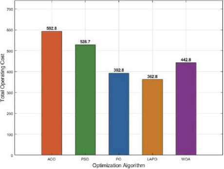
Figure 7 Electricity costs for small users.
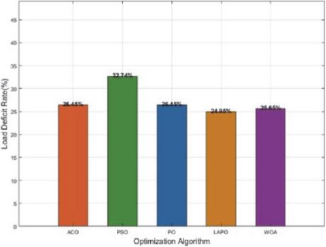
Figure 8 Load deficit rates for small users.
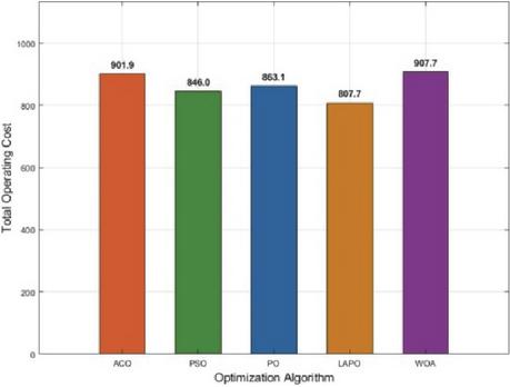
Figure 9 Electricity costs for larger users.
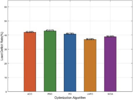
Figure 10 Load deficit rates for larger users.
In the small-user microgrid dispatch scenario depicted in Figure 7, the operational costs of the four optimization algorithms exhibit a significant gradient difference: the ACO algorithm incurs the highest cost, followed by the PSO algorithm. The PO algorithm reduces costs to 392.8 yuan, whereas the LAPO algorithm achieves the optimal cost of 362.8 yuan. Comparatively, the LAPO algorithm reduces costs by approximately 38.8% compared with ACO and by 7.6% compared with the second-best PO algorithm. Under small-user load fluctuation scenarios, it more precisely matches the output constraints of low-cost power sources such as PV and energy storage, reducing the reliance on high-cost grid electricity purchases.
In the small-user microgrid dispatch scenario depicted in Figure 8, the load-deficit rates of the four algorithms distinctly differ: the ACO algorithm results in the highest deficit rate, followed by the PSO algorithm. The PO algorithm reduces the deficit rate to 28.42%, whereas the LAPO algorithm achieves the lowest deficit rate at 24.45%. LAPO’s advantage lies in its precise adaptation to supply unit constraints: when confronting small users’ load fluctuations, it optimally schedules energy storage and grid power purchases. This approach maintains the lower limits of PV and wind power generation while minimizing supply gaps. Compared with ACO, LAPO reduces the power shortage rate by 13.97%. Even against the second-best PO algorithm, it further lowers the power shortage risk by 4%. This demonstrates LAPO’s superiority in achieving a low-cost power supply with high reliability assurance, making it better suited to small users’ demand for stable electricity.
In the large-user microgrid scheduling scenario shown in Figure 9, the operational costs of the four algorithms differ significantly: PO incurs the highest cost, followed by ACO. PSO reduces costs to 834.9 yuan, whereas LAPO achieves the optimal cost at 807.1 yuan. When the peak-to-valley load difference for large users reaches 120 kW, LAPO leverages its enhanced multitime-slot coordination optimization capability to precisely match the low-cost output from PV and energy storage with load fluctuations. Compared with the PO algorithm, it reduces costs by 19.1%, and compared with the PSO algorithm, it reduces costs by 3.3%. This advantage stems from LAPO’s precise control over high-cost grid power purchases. While ensuring large users’ electricity needs, it maximizes the utilization of distributed power sources’ low-carbon and low-cost characteristics, demonstrating its scheduling superiority in complex scenarios.
In the large-user microgrid dispatch scenario depicted in Figure 10, the load shortfall rates of the four algorithms exhibit a clear gradient: ACO shows the highest shortfall rate, followed by PSO. PO reduces the rate to 39.34%, whereas the LAPO algorithm achieves the lowest shortfall rate at 38.84%. When the large user’s peak load reached 170 kW, LAPO reduced the power shortage rate by 3.68% compared with ACO and by 0.5% compared with PO. This demonstrates LAPO’s superior alignment with large users’ core requirements for power stability in complex, extended-duration scenarios.
7 Conclusion
A scheduling method for microgrids based on the parrot optimization algorithm with chaotic and adaptive weighting has been proposed. This approach enhances population diversity by incorporating logistic chaos principles and balances global and local exploration capabilities through adaptive weight adjustment strategies, thereby effectively improving algorithm performance. Favorable results in microgrid scheduling have been demonstrated. Moving forward, we aim to construct more complex microgrid scheduling models while further optimizing algorithm performance.
References
[1] P. Arévalo, D. Benavides, D. Ochoa-Correa, et al., ‘Smart Microgrid Management and Optimization: A Systematic Review Towards the Proposal of Smart Management Models’, Algorithms, Vol. 18, No. 7, pp. 429. July, 2025.
[2] J. Vaish, A.K. Tiwari, K.M. Siddiqui, ‘Optimization of micro grid with distributed energy resources using physics based meta heuristic techniques’, IET Renewable Power Generation, Vol. 19, no. 1, pp. e12699. February, 2025.
[3] R. Rishabh, K.N. Das, ‘A critical review on metaheuristic algorithms based multi-criteria decision-making approaches and applications’, Archives of Computational Methods in Engineering, Vol. 32, No. 2, pp. 963–993, March, 2025.
[4] J. Lian, G. Hui, L. Ma, et al., ‘Parrot optimizer: Algorithm and applications to medical problems’, Computers in Biology and Medicine, Vol. 172, pp. 108064. April, 2024.
[5] J. Martinez-Rico, E. Zulueta, I.R. de Argandoña, et al., ‘Multi-objective optimization of production scheduling using particle swarm optimization algorithm for hybrid renewable power plants with battery energy storage system’, Journal of modern power systems and clean energy, Vol. 9, No. 2, pp. 285–294, March, 2021.
[6] L.L. Li, B.X. Ji, G. C. Liu, et al., ‘Grid-connected multi-microgrid system operational scheduling optimization: A hierarchical improved marine predators algorithm’, Energy, Vol. 294, pp. 130905, May, 2024.
[7] A. Dong, S. K. Lee, ‘The Study of Scheduling Optimization for Multi-Microgrid Systems Based on an Improved Differential Algorithm’, Electronics, Vol. 13, No. 22, pp. 4517, November, 2024.
[8] A. Kheiter, S. Souag, A. Chaouch, et al., ‘Energy management strategy based on marine predators algorithm for grid-connected microgrid’, International Journal of Renewable Energy Development, Vol. 11, No. 3, pp. 751–765, May, 2022.
[9] L. Yuwei, L. Li, L. Jiaqi, ‘Hybrid scheduling strategy and improved marine predator optimizer for energy scheduling in integrated energy system to enhance economic and environmental protection capability’, Renewable Energy, Vol. 228, pp. 120641, July, 2024.
[10] M. R. Zhou, M. Zhou, F. Hu, et al., ‘Optimization of Microgrid Scheduling with Electric Vehicles Based on Improved Hiking Optimization Algorithm’, The 10th Asia Conference on Power and Electrical Engineering (ACPEE). IEEE, pp. 710–714, April, 2025.
[11] L. Wen, K. Zhou, S. Yang, et al., ‘Optimal load dispatch of community microgrid with deep learning based solar power and load forecasting’, Energy, Vol. 171, pp. 1053–1065, March, 2019.
[12] A. B. Ghorbal, A. Grine, I. Elbatal, et al., ‘Predicting carbon dioxide emissions using deep learning and Ninja metaheuristic optimization algorithm’, Scientific Reports, Vol. 15, No. 1, pp. 4021–4048, February, 2025.
[13] J. Chen, N. Hu, ‘Distributed Optimization Model for Economic Dispatch of Smart Grid’, Distributed Generation & Alternative Energy Journal, Vol. 40, Issue 3, pp. 457–480, July, 2025.
[14] L. Pan, X. Yang, Y. Fu, et al., ‘Distribution Network Scheduling Model Taking Into Account Power Generation Prediction of New Energy and Flexible Loads’, Distributed Generation & Alternative Energy Journal, Vol. 40, Issue 2, pp. 401–426, April, 2025.
[15] A.A.Z. Diab, A.M. El-Rifaie, M. M. Zaky, et al., ‘Optimal sizing of stand-alone microgrids based on recent metaheuristic algorithms’, Mathematics, Vol. 10, No. 1, pp. 140. January, 2022.
[16] A. Bouaouda, Y. Sayouti, ‘An optimal sizing framework of a microgrid system with hydrogen storage considering component availability and system scalability by a novel approach based on quantum theory’, Journal of Energy Storage, Vol. 92, pp. 111894, July, 2024.
[17] S. F. Castellanos-Buitrago, P. Maya-Duque, W. M. Villa-Acevedo, et al., ‘Enhancing Energy Microgrid Sizing: A Multiyear Optimization Approach with Uncertainty Considerations for Optimal Design’, Algorithms, Vol. 18, No. 2, pp. 111, February, 2025.
[18] M. S. Islam, T. K. Roy, I. J. Bushra, ‘Marine predators algorithm-based robust composite controller for enhanced power sharing and real-time voltage stability in DC–AC microgrids’, Algorithms, Vol. 18, No. 8, pp. 531. August, 2025.
[19] G. Abdi, M.A. Jirdehi, H. Mehrjerdi, ‘Optimal coordination of overcurrent relays in microgrids using meta-heuristic algorithms NSGA-II and harmony search’, Sustainable Computing: Informatics and Systems, Vol. 43, pp. 101020. September, 2024.
[20] Z. Xiong, Z. Cai, Q. Lai, ‘Cloud-Edge Collaborative Control Technology for Power Grid Construction Based on Holographic Digitization’, Distributed Generation & Alternative Energy Journal, Vol. 40, Issue 5&6, pp. 947–972, December, 2025.
[21] P. Kasap, A. O. Faouri, ‘Comparison of the meta-heuristic algorithms for maximum likelihood estimation of the exponentially modified logistic distribution’, Symmetry, Vol. 16, No. 3, pp. 259, February, 2024.
[22] H.M. Saatchi, A.A. Khamseh, R. Tavakkoli-Moghaddam, ‘Solving a new bi-objective model for relief logistics in a humanitarian supply chain using bi-objective meta-heuristic algorithms’, Scientia Iranica. Transaction E, Industrial Engineering, Vol. 28, No. 5, pp. 2948–2971, January, 2021.
[23] P. S. Naulia, J. Watada, I.A. Aziz, ‘A mathematically inspired meta-heuristic approach to parameter (weight) optimization of deep convolution neural network’, IEEE Access, Vol. 12, pp. 83299–83322, June, 2024.
[24] P. Majumdar, S. Mitra, ‘Enhanced honey badger algorithm based on nonlinear adaptive weight and golden sine operator’, Neural Computing and Applications, Vol. 37, No. 1, pp. 367–386, January, 2025.
Biography

Yan Li received her bachelor’s degree in computer science and technology from Zhengzhou University in 2005 and her master’s degree in computer software and theory from Zhengzhou University in 2008. She is currently a lecturer in the Construction Information Engineering Department of HeNan Technical College of Construction, and her research interests are computer networks, computer applications, big data and cloud computing.
Distributed Generation & Alternative Energy Journal, Vol. 41_2, 327–354
doi: 10.13052/dgaej2156-3306.4124
© 2026 River Publishers