Optimisation of Emergency Power Restoration in Distribution Networks with Distributed Generation Integration
Lehui Lin1 and Jifang Li2,*
1Dongbei University of Finance and Economics, Dalian 116025, People’s Republic of China
2Meizhou Power Supply Bureau of Guangdong Power Grid Co., Ltd., Meizhou 514000, Guangdong, China
E-mail: itlywork@126.com; jifangli2526@outlook.com; 3716677@163.com
*Corresponding Author
Received 13 January 2026; Accepted 10 April 2026
Abstract
The integration of distributed generation (DG) such as photovoltaic and wind power systems into distribution networks significantly alters power flow patterns and operational characteristics, introducing stochasticity and uncertainty into voltage and loss behavior. Higher-order semi-invariants (cumulants) yield greater accuracy and computational efficiency than traditional Monte Carlo simulations; therefore, they can be employed as the preferred and more reliable method of performing effective stochastic power flow analysis of very complex power systems. Meanwhile, wiring errors at the user side, such as neutral-to-earth misconnection, compromise residual current device (RCD) protection and elevate electric shock risks. Feeder clustering via the CFSFDP algorithm is integrated with this stochastic loss modeling framework to identify user groups and isolate faulty users, providing a cohesive methodological approach for practical distribution network analysis. An analysis performed on wiring error hazard mechanisms and the associated ground scheme’s performance against RCDs; examining the stochastic power flow and line loss distribution models by utilizing higher-order cumulative distributions for evaluating the voltage and loss statistical distributions. Cumulative distribution methodologies have been shown to have an order of magnitude less compute time than Monte Carlo simulation and equivalent performance accuracy. The user grouping algorithm developed in this study (CFSFDP) does not require the specification of input cluster(s) to create a grouping. Fault localization is accomplished through an adaptive lasso-type model. The method developed for validating the algorithms used in this study on the IEEE 34 Bus network have shown to be very accurate and efficient.
Keywords: Distributed generation, stochastic power flow, semi-invariants, feeder clustering, residual current, faulty user localization.
1 Introduction
In recent years, with the large-scale deployment of distributed generation (DG) such as photovoltaic and wind power systems, the topology and operating characteristics of power distribution networks have undergone profound changes [1, 2]. Distributed generation, by virtue of its proximity to load centers, low-carbon footprint, and scalability, plays an increasingly critical role in enhancing grid resilience and supporting the global transition toward renewable energy. However, the inherent intermittency and randomness of DG outputs introduce significant uncertainties to the power flow and loss characteristics of distribution networks [3]. Moreover, the massive integration of DG into low-voltage distribution networks increases the complexity of operation and maintenance, particularly in rural and urban communities where user-side wiring errors and protection device misconfigurations are not uncommon. Against this backdrop, assessing the impact of DG access on feeder clustering, power losses, and protection reliability becomes an essential research direction [4].
Specifically, in low-voltage distribution systems, improper user wiring – such as the interchange of neutral and protective earth conductors – can compromise the effectiveness of residual current devices (RCDs) and undermine the three-tier protective barrier designed to prevent electric shock accidents. Safety and operational problems may occur when customers are incorrectly wired into low-voltage distribution networks. Wiring faults create elevated touch voltages, unintended residual current flow through the circuit, and incorrect operation or failure to operate [rest], respectively, RCDs. Moreover, faults may sometimes propagate throughout the network, affecting multiple customers, which will increase the chance of electric shock hazards and widespread failures of protective measures (i.e., RCDs). Ultimately, the identification and mitigation of potential impacts from these types of wiring faults is essential to maintaining the safety and reliability of current distribution systems. Studies have shown that under TT, TN-S, and TN-C-S grounding systems, the presence of improperly wired users can lead to excessive residual currents that repeatedly trip RCDs, elevate touch voltages on appliance enclosures, and amplify the risk of widespread electric shock incidents across all users sharing the same protective earth [5, 6]. This underscores the critical need to understand the mechanisms of residual current propagation and the role of feeder clustering in isolating faulty users to enhance safety.
The effectiveness of grounding systems (TT, TN-S and TN-CS), and therefore the ability of residual current devices (RCDs) to operate safely, depends on the ability of RCDs to operate safely as the grid evolves. Today’s distribution networks with higher levels of distributed generation (DG), more bi-directional currents, and different fault current paths can have a large impact on how RCDs respond. These issues could potentially reduce the sensitivity of RCD fault detection or can result in delayed tripping of RCD protection devices. As a result, it is important to gain an understanding of the interactions between grounding configurations and uncertainties caused by DG to ensure continued reliable fault detection and protective performance of the RCDs.
On the other hand, DG integration alters the power flow and voltage profile of feeders by injecting active and reactive power locally. While DG can alleviate upstream transformer loading and reduce line losses under favorable matching conditions, it can also increase voltage fluctuation, reverse power flow, and induce greater uncertainty in line losses due to the stochastic nature of renewable energy outputs. Consequently, it becomes imperative to develop computationally efficient and accurate models for stochastic power flow and loss evaluation in large-scale distribution networks [7, 8].
Challenges arise from two main aspects. First, the modeling of stochastic power flow requires repeated convolutions of random variables representing the uncertain outputs of DG and loads, which are computationally intensive, especially for large networks. Monte Carlo simulation (MCS), despite its robustness, suffers from prohibitively high computational cost in practical applications [9]. Second, identifying and isolating faulty users with improper wiring in a dense low-voltage network remains technically challenging due to the complex correlation between residual currents and individual user loads, compounded by measurement noise and missing data.
In the literature, various methods have been proposed to address these challenges. Stochastic power flow methods based on cumulants, polynomial chaos expansion, and point estimation techniques have been investigated as alternatives to MCS to improve computational efficiency [10]. Cumulant-based methods, in particular, leverage the additivity of cumulants (semi-invariants) to simplify the calculation of sums of independent random variables, thereby accelerating the evaluation of voltage and loss distributions under uncertainty. Similarly, clustering algorithms such as k-means, hierarchical clustering, and density-based spatial clustering (DBSCAN) have been applied to identify homogeneous feeder segments or user clusters based on load profiles, but they often suffer from sensitivity to initial conditions and difficulty in determining the number of clusters a priori. Furthermore, approaches based on association rule mining, such as the Apriori algorithm, have been used to extract correlations between abnormal currents and user behavior, but they tend to generate excessive, non-informative rules and require extensive post-processing [11, 12].
However, existing methods still exhibit several shortcomings. The cumulant-based stochastic power flow models often consider only lower-order moments, which may be insufficient to capture the tail behavior of line losses under high-penetration DG scenarios. Clustering methods often lack robustness in the presence of complex, irregular data distributions and fail to adequately exploit local density variations to identify meaningful clusters. Faulty user identification techniques frequently overlook the effects of multicollinearity among user loads and are not robust to missing or noisy measurements [13].
To overcome these limitations, this paper proposes an integrated Faulty User Localization for feeder clustering and stochastic loss impact assessment in distribution networks with DG integration. The key contributions of this work are as follows:
We analyze the mechanisms and hazards of wiring errors in low-voltage distribution systems under various grounding schemes (TT, TN-S, and TN-C-S) and elucidate how faulty users compromise the effectiveness of RCD protection layers, leading to elevated residual currents and increased electric shock risk.
We develop a stochastic power flow and line loss computation framework based on higher-order semi-invariants (cumulants), which improves accuracy in capturing the probabilistic characteristics of network parameters while significantly reducing computational burden compared to MCS. We also derive closed-form relationships between moments, central moments, and cumulants to facilitate practical implementation [14, 15].
To improve the feeder clustering process, we employ the Clustering by Fast Search and Find of Density Peaks (CFSFDP) algorithm, which effectively identifies cluster centers based on local density and relative distance without requiring a priori knowledge of the number of clusters. This enables more reliable identification of homogeneous user groups with similar load and residual current characteristics.
We implement an adaptive Lasso regression model for faulty user localization, capable of isolating individual or multiple faulty users even under scenarios with missing measurement data and correlated user loads. The model’s hyperparameters are tuned via cross-validation, and its performance is validated through synthetic experiments.
2 Risk Mechanisms of Distribution System Wiring Errors
2.1 Fault Hazard Mechanism
In the low-voltage residential power supply system, according to the differences in grounding and electrical protection methods, it is usually categorized into three typical forms: TT system, TN-S system and TN-C-S system. Each type of system has different ways of hierarchical configuration of RCD in the design, and its layout structure can be referred to as shown in Figure 1. Different grounding methods directly affect the path of fault current and the reliability of RCD action, so when analyzing the potential hazards caused by wiring errors, it is necessary to combine with the type of power supply system and its protection mechanism to make specific judgments.
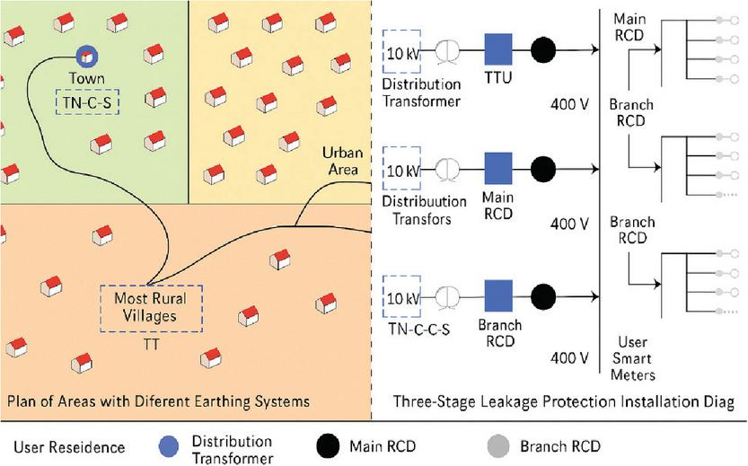
Figure 1 RCD deployment structures in TT, TN-S, and TN-C-S systems.
In low-voltage distribution systems, common grounding methods include the three-phase four-wire system (often used in rural areas), the TN-S system, and the TN-C-S system.
1. In the three-phase four-wire system, the neutral point of the distribution transformer is directly grounded, and the enclosures of electrical appliances are grounded independently. In practice, one or more households may share the same protective earth (PE) conductor. This configuration is prevalent in rural distribution networks.
2. The TN-S system uses a three-phase five-wire arrangement, where the neutral (N) and PE conductors are separately derived from the transformer and remain isolated throughout. This setup effectively avoids voltage interference between N and PE lines and is commonly used in urban power supply systems.
3. The TN-C-S system features a hybrid layout, with a three-phase four-wire configuration at the power source side and separate N and PE conductors derived near the user load. Since the N and PE conductors are bonded at the power source, primary-level RCDs (Residual Current Devices) cannot be installed; only secondary and tertiary RCDs can be deployed for protection.
In these grounding systems, if user-side wiring errors occur, the resulting load current will fluctuate regularly depending on appliance usage patterns. During off-peak periods, when high-power devices are in standby or off, the residual current in the transformer service area typically remains below 300 mA. However, during peak usage, when such devices are switched on, the branch and total residual current may significantly exceed 300 mA. If no tertiary RCD is installed at the affected user’s premises, the upstream RCDs may trip frequently, disrupting the power supply to the entire area.
Table 1 Comparative analysis of TT, TN-S, and TN-C-S grounding systems
| Feature | TT System | TN-S System | TN-C-S System |
| Neutral & Earth Configuration | Separate earth electrode, independent grounding | Separate N and PE throughout system | Combined PEN at source, separated near load |
| Typical Application | Rural/isolated areas | Urban/industrial systems | Residential & commercial distribution |
| RCD Installation | Full tier (primary, secondary, tertiary) | Full tier possible | Primary not possible, only secondary & tertiary |
| Fault Current Path | Through local earth electrode | Through dedicated PE conductor | Through combined PEN conductor |
| Safety Level | High (independent grounding) | Very high (clear separation) | Moderate (risk if PEN fails) |
| Key Risk | High earth resistance issues | Minimal interference | PEN failure leads to shock risk |
Table 1 summarizes the key features of three types of electrical grounding systems, TT, TN-S & TN-C-S. These include the configuration of their neutral and protective earth, their typical application, the installation of RCDs, the path of fault current and their associated safety issues to provide a quick reference for comparing the differences between each system.
To ensure electrical safety and prevent electric shock incidents, a three-layer protection mechanism is essential: correct deployment of tiered RCDs, reliable disconnection of fault circuits by the RCDs, and effective grounding that limits the voltage of exposed conductive parts. In a TT system, if the neutral and earth lines are mistakenly connected, the user’s load current (Id) will flow through the PE conductor into the ground, forming a return path through the transformer neutral. Prolonged high current in the PE line may damage connectors and increase ground resistance, causing hazardous touch voltage (U_touch) on the enclosures of all devices connected to that PE line.
Since the voltage on the equipment enclosures originates from the PE line itself, even properly installed tertiary RCDs may fail to provide protection. This compromises the entire electric shock prevention system. Customers who are incorrectly wired in low-voltage distribution systems have serious safety and operational risks. Miswiring can cause unwanted current paths through protective earth conductors resulting in higher-than-normal touch voltages, frequent or erroneous tripping of RCDs, and potential damage to connectors or other equipment. The hazards of mis wired systems impact the safety of the individual customer, and other customers who use the same protective earth network as the mis wired customer; ultimately underscores the need for proper installation and the deployment of tiered RCDs in order to provide adequate protection for all users within the network. A single user’s wiring error can expose all other users on the same PE network to elevated risk, significantly increasing the likelihood and severity of electric shock accidents. Figure 2 shows schematic showing how incorrect user wiring redirects current through the protective earth, increasing touch voltage and fault risk.
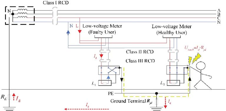
Figure 2 Schematic showing how incorrect user wiring redirects current through the protective earth, increasing touch voltage and fault risk.
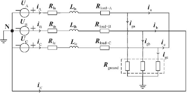
Figure 3 Residual current monitoring and analysis module showing how RCDs detect leakage faults and how miswiring affects readings.
2.2 Fault Mechanism Analysis
Figure 3 illustrates the operational principle of a primary RCD, which relies on differential current sensing to detect leakage faults. The core function of an RCD is to continuously monitor the vector sum of the currents in the live (L) and neutral (N) conductors. This sum represents the residual current , which can be expressed mathematically as:
| (1) |
Where is the current flowing through the live conductor, is the current returning through the neutral conductor (considered negative in direction).
Under normal operating conditions, assuming no ground leakage, the incoming and outgoing currents are equal in magnitude but opposite in direction:
| (2) |
However, when a leakage fault occurs – such as current flowing to earth through a human body or damaged insulation – a portion of the current bypasses the neutral path. The new condition becomes:
| (3) |
If Ires exceeds a predefined threshold (e.g., 30 mA, 100 mA, or 300 mA), the RCD will trip:
| (4) |
In the case of incorrect wiring, particularly when the neutral conductor is mistakenly bonded to the PE line at the load side, a portion of the return current may flow through PE instead of N. As a result, the differential current measurement is distorted. The RCD may calculate:
| (5) |
If , then:
| (6) |
This leads to false negatives, where dangerous leakage currents remain undetected. Moreover, the long-term flow of load current through PE may heat connectors, increase the ground resistance, and elevate touch voltages on equipment enclosures:
| (7) |
Where is the effective grounding resistance. If exceeds safety thresholds (typically 50 V in dry environments), users are at risk of electric shock even when a tertiary RCD is present.
Consider a three-phase low-voltage power distribution system. Let denote the phase current flowing through the user loads connected to phases A, B, and C respectively. Normally, the return current from these loads flows through the neutral conductor back to the transformer. However, if a user has incorrectly wired the neutral and protective earth conductors, the return path shifts to the grounding system, leading to unintended current in the PE conductors [16, 17].
Let represent the current flowing through the PE line corresponding to each phase. In such a miswiring scenario, the current balance equations for the system can be expressed as:
| (8) | |
| (9) | |
| (10) |
Assuming that the neutral current is absent due to miswiring (i.e., the return path is fully diverted to PE), the residual current detected by the RCD in the distribution transformer area can be written as:
| (11) |
Substituting (8)–(10) into (12), we obtain:
| (12) |
However, this cancellation only holds if all PE return currents are measured correctly by the RCD, which is rarely the case in real-world systems. In practical deployments, especially at the transformer area level, RCDs typically monitor only the phase and neutral conductors, not the PE path. As a result, the actual measurement becomes:
| (13) |
And since due to the open neutral, while PE currents bypass the RCD, we effectively have:
| (14) |
This leads to a significant overestimation of residual current, which may exceed the threshold of both primary and secondary RCDs (e.g., 300 mA), causing them to trip repeatedly or refuse to engage (lockout) due to perceived persistent leakage.
3 Properties of Cumulants and Their Application in Stochastic Power Flow Calculations
Stochastic power system analysis commonly considers the uncertainty associated with load and generation from distributed sources as a probabilistic variable and uses Probability Theory to describe these uncertain loads and distributed generation. The statistical moments (mean/average, variance, etc.) of the random variables are used to provide a description of the basic shape of the distribution of measurements on those random variables, but they cannot adequately describe all of the potentially non-Gaussian shapes of the distributions. Higher order statistical moments, especially cumulants, provide a better overall representation of the uncertainty involved because higher order cumulants allow for a more complete statistical representation of probabilistic power flow, including line losses, resulting from a complex distribution network.
With the widespread integration of distributed generation, the output of power sources in distribution networks exhibits significant intermittency and volatility. Meanwhile, the stochastic nature of loads introduces considerable uncertainty in the system’s operational parameters. This uncertainty directly impacts the distribution of power flows and line losses, making traditional deterministic analysis methods inadequate to accurately represent actual operating conditions [18].
To characterize the stochastic fluctuations of line losses in distribution networks, stochastic power flow methods are employed to perform statistical analysis on operational parameters and line losses. Essentially, stochastic power flow involves the convolution of multiple random variables to obtain the probability distribution functions of system state variables, such as nodal voltages, branch flows, and line losses.
However, convolution operations typically require substantial computational resources and time, becoming the main bottleneck in stochastic power flow calculations. To improve computational efficiency, this study introduces the cumulant method, which leverages the advantageous properties of cumulants to simplify the convolution of random variables [19, 20].
Let X be a random variable with moment generating function (MGF) defined as . The cumulant generating function (CGF) is the logarithm of the MGF:
| (15) |
where denotes the n-th order cumulant. Cumulants have the following key properties:
• Additivity: For independent random variables X and Y, the cumulant generating function of their sum satisfies
| (16) |
This property converts the convolution of multiple random variables into a simple summation of cumulants, greatly simplifying calculations.
• Relation to Moments: There are explicit conversion formulas between moments and cumulants, enabling flexible usage in practical computations.
Based on these properties, the cumulants of the aggregate stochastic variable in the distribution network satisfy
| (17) |
Using this, the probabilistic parameters of line losses L can be obtained by summing the cumulants of each contributing random variable, thus avoiding complex high-dimensional convolutions and significantly accelerating computation.
In summary, the cumulant method not only enables fast computation of stochastic power flows and extreme line losses in large-scale distribution networks but also provides theoretical support and practical tools for uncertainty analysis in power systems.
3.1 Definition and Properties of Cumulants
Cumulants are numerical characteristics of random variables and serve as a fundamental concept in probability theory and mathematical statistics. They provide an alternative to moments for describing distributions, especially useful for analyzing sums of independent random variables [21].
Let T be a random variable with distribution function . Suppose iii is a real number and the function is integrable over (). The characteristic function of the real-valued random variable T is defined as
| (18) |
where denotes the expectation operator, , and is a real variable.
The cumulant generating function (CGF) is defined as the natural logarithm of the characteristic function:
| (19) |
Expanding as a power series around zero yields
| (20) |
where denotes the n-th order cumulant of T.
Key properties of cumulants include:
• Additivity: For independent random variables X and Y, the cumulant of their sum satisfies
| (21) |
• Relation to Moments: Cumulants can be expressed in terms of moments, and vice versa, allowing flexible statistical characterization.
• Zero for Independent Components: If certain moments vanish, the cumulants reflect this, often simplifying the analysis.
In stochastic power flow computations, the cumulant method leverages these properties to transform convolutions of distributions (i.e., sums of random variables) into simple cumulant additions, accelerating computations and enabling effective analysis of distribution network uncertainties.
3.2 Moments and Central Moments
Given the probability distribution of a random variable, one can calculate its moments and central moments, which serve as fundamental statistical measures describing the variable’s distribution characteristics.
For a continuous random variable Z with probability density function (PDF) , the n-th order raw moment is defined as:
| (22) |
Here, denotes the expectation operator, and n is a positive integer indicating the moment’s order.
The central moment of order n, denoted , measures the moments about the mean and is given by:
| (23) |
where is the mean (first moment) of Z.
Central moments are particularly useful because they provide information about the distribution’s shape relative to its mean: The second central moment is the variance, quantifying dispersion. The third central moment relates to skewness, indicating asymmetry. The fourth central moment relates to kurtosis, describing tail heaviness.
For discrete random variables, moments and central moments can be computed similarly by replacing integrals with summations over the probability mass function (PMF).
In this work, these moment definitions serve as the basis for further analysis of uncertainties in distribution network flows and losses.
3.3 Calculation of Cumulants
Similar to moments, cumulants are numerical characteristics of a random variable that capture essential distributional features. Each cumulant of a given order can be expressed as a function of moments of the same or lower orders.
In this section, we will use a consistent notation for each type of moment/cumulant. The n-th order cumulant will be written as and the n-th order moment as Let represent the first two the second and the n-th order moments respectively. Similarly, the first two the n-th order cumulants are denoted by and and . This standardization ensures that the symbols remain consistent across all equations which prevents confusion while maintaining mathematical clarity. The relationships between cumulants and moments are expressed using these standardized notations throughout this subsection.
Let denote the n-th order cumulant, and represent the k-th order moment. The relationship between cumulants and moments can be established through recursive formulas or generating functions.
For instance, the first few cumulants are related to moments as follows:
| (24) | |
| (25) | |
| (26) | |
| (27) |
These cumulants provide insight into key properties of the distribution: : mean, : variance, : skewness-related measure, : kurtosis-related measure.
The high-order cumulants expressed in (24)–(27) provide important components in determining the statistical behavior of stochastic line losses. The second cumulant (variance) defines the degree to which line losses disperse around their mean value, as well as indicating the level of uncertainty within the system. The third cumulant (skewness) defines how symmetrical or asymmetrical the probability distribution of line losses is; i.e., whether there is a greater likelihood of experiencing higher or lower line loss. Finally, the fourth cumulant (kurtosis) represents how extreme the values of line losses are, as well as how likely it is to experience large-scale losses, even if they’re infrequently occurring events. Using these high-order cumulants to estimate probable (i.e., “typical”) and extreme deviations in line losses will improve the prediction accuracy and reliability of line loss models developed using this methodology, whether operating under “normal” or “extreme” operating conditions.
Generally, calculating cumulants up to the seventh order () suffices to ensure an accurate representation of the random variable’s characteristics in practical applications.
The cumulants are crucial in stochastic power flow computations since they allow efficient convolution of random variables and reduce computational complexity when analyzing distribution network losses under uncertainty.
4 Stochastic Power Flow and Line Loss Calculation Based on Cumulants
Stochastic power flow analysis extends the conventional deterministic linear power flow calculations by incorporating the probabilistic characteristics of input variables. Through convolution operations, it computes the PDF and cumulative distribution functions (CDFs) of state variables such as node voltages and branch currents. Compared to traditional power flow methods, stochastic power flow better captures the dynamic and uncertain nature of power systems, especially with increasing integration of intermittent distributed energy resources [22, 23].
4.1 Detailed Derivation of Cumulants for Power Output
Assume that the generator output PPP is a discrete random variable with multiple possible output states , each occurring with probability , where , and satisfying:
| (28) |
Step 1: Calculate Raw Moments Raw moments are expectations of powers of the random variable, defined as:
| (29) |
where is the order of the moment. The meanings are:
The first-order moment is the mean (expected value):
| (30) |
The second-order moment m2m_2m2 is the expected value of the square:
| (31) |
Higher order moments describe more detailed statistical characteristics.
Step 2: Calculate Central Moments Central moments measure deviations relative to the mean:
| (32) |
Central moments describe variance, skewness, kurtosis, etc.:
The second central moment is the variance:
| (33) |
The third central moment measures skewness, indicating asymmetry of the distribution.
Step 3: Aggregation of Cumulants for Multiple Generators Suppose there are M independent generators in the system, with cumulants for the j-th generator, where .
Then, the k-th order cumulant of the total power output is:
| (34) |
By the above steps, the statistical characteristics of random generator outputs are precisely described by cumulants. Utilizing the additive nature of cumulants, the impact of stochastic power injections on voltages, power flows, and line losses in distribution networks can be efficiently calculated.
4.2 Cumulants of Distribution Network Power Losses
In the analysis of distribution systems, power losses arise due to the difference between the total injected power and the total output power delivered to the loads. This net loss, which fluctuates due to the stochastic nature of generation and demand, can be quantitatively described using cumulants (semi-invariants) of the associated random variables [24].
Let: denote the total injected power in the system; denote the total delivered (output) power to the loads; represent the total power loss in the network.
Since both and are modeled as random variables with known probability distributions (based on generation variability and load uncertainty), the distribution of can be derived from their statistical characteristics.
Step 1: Deriving the Cumulants of Power Loss According to the additive and subtractive properties of cumulants:
| (35) |
Where: represents the n-th order cumulant, The sign accounts for the subtraction in the random variable difference .
This formula implies:
• First-order cumulant (mean):
| (36) |
• Second-order cumulant (variance):
| (37) |
• Third-order cumulant (skewness-related):
| (38) |
• and so on.
Step 2: Interpretation and Use This cumulant formulation allows for the rapid estimation of the statistical distribution of power losses without relying on computationally expensive numerical convolution. Especially in large-scale distribution networks with multiple variable energy sources and loads, this technique: Captures the uncertainty propagation through the network, facilitates risk-based decision-making and planning, enables fast stochastic load flow computation using only statistical descriptors.
Once the cumulants of power losses are obtained, techniques like the Edgeworth Expansion or Gram–Charlier Series can be applied to reconstruct approximate PDF for the power loss.
5 Scene Reduction Based on the CFSFDP Clustering Algorithm
In order to reduce the computational complexity in probabilistic analysis, scene reduction is employed to retain representative scenarios from a large dataset. The CFSFDP (Clustering by Fast Search and Find of Density Peaks) algorithm provides an efficient and shape-agnostic method to identify cluster centers and assign other points accordingly, making it especially suitable for scene reduction in complex datasets.
This method is based on the assumption that cluster centers exhibit higher local density and are relatively distant from other points with higher density. These two criteria help distinguish cluster centers from peripheral points.
Step 1: Compute Local Density For each data point ii, the local density is calculated as:
| (39) |
Where: is the Euclidean distance between points i and j, is the cut-off distance (typically chosen to ensure a certain average number of neighbours), is an indicator function:
| (40) |
This means represents the number of points that lie within distance from point ii, acting as a proxy for local density.
Step 2: Compute Minimum Distance to Higher-Density Points For each point i, compute as the minimum distance to any point j with a higher local density:
| (41) |
If point ii has the highest local density (i.e., no other point has ), then:
| (42) |
This step ensures that true cluster centers not only have high density but are also isolated from other high-density areas.
Step 3: Identify Cluster Centers A decision graph is plotted using and as axes. Points that have both high and high are selected as cluster centers.
Typically, a threshold is set, or an elbow method is used to choose the number of centers kk based on prominent peaks in the graph.
Step 4: Assign Remaining Points Each non-center point is assigned to the same cluster as its nearest neighbor j with higher density:
| (43) |
This guarantees that points are grouped by proximity and density hierarchy.
Step 5: Select Representative Scenes Once the dataset is divided into clusters, the cluster center or a weighted average point within each cluster can be chosen to represent the entire cluster. This reduces the scenario space while retaining the statistical characteristics of the original data.
This approach allows for efficient and explainable scene reduction, crucial in probabilistic power flow analysis, renewable forecasting, or uncertainty quantification in energy systems.
Let me know if you’d like visual aids (e.g., decision graph or sample cluster plots), or if you want this written in LaTeX or translated into Chinese.
6 Case Study and Validation
6.1 Overview of the Case Example
To validate the effectiveness and accuracy of the proposed extreme line loss assessment method based on semi-invariants, a simulation was conducted on the widely recognized IEEE 34-node test feeder. This distribution system serves as a standard benchmark in the field of power system analysis due to its inclusion of realistic features such as long radial structures, unbalanced loading, and voltage regulation components [25].
The IEEE 34-node feeder was chosen due to being well known, its radial topology and unbalanced load conditions that allow good evaluation of the cumulant-based stochastic line loss modeling approach. The physical structure of the feeder and variety of load types simulated provide realistic operational challenges for evaluating the accuracy and effectiveness of the proposed method in performing under stochastic conditions.
The network’s topology is depicted in Figure 4, which illustrates the radial layout of the feeder, complete with lateral branches and varying line lengths. This test system incorporates a mix of load types, including residential, commercial, and light industrial customers, providing a realistic foundation for evaluating line losses under stochastic power flow conditions.
In the simulation, uncertainties from both distributed generation outputs (e.g., PV and wind) and stochastic load variations were introduced to emulate real-world operational volatility. The goal is to use the semi-invariant-based stochastic power flow approach to capture the probability characteristics of line losses, particularly under extreme or rare-event scenarios.
Key modeling steps include: Assigning probabilistic distributions to each node’s load and DG output. Computing the statistical moments (mean, variance, skewness, etc.) of power injections. Applying the semi-invariant convolution method to obtain the distribution and CDF of total system losses. Comparing results against Monte Carlo simulations to verify computational efficiency and accuracy.
The results of this case study not only highlight the feasibility of using semi-invariant techniques for loss modeling in active distribution networks but also demonstrate substantial computational advantages, especially when dealing with large-scale scenarios or time-constrained planning environments.
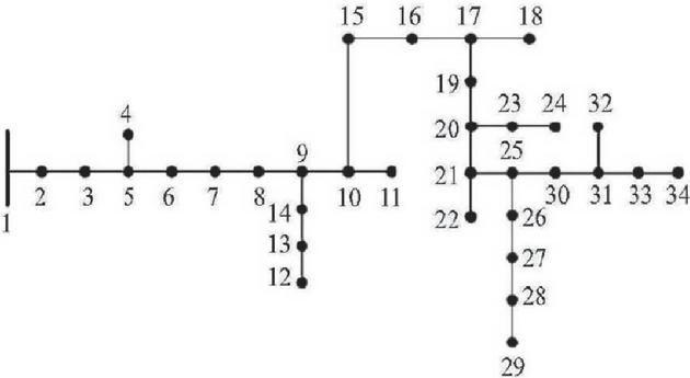
Figure 4 IEEE 34-node distribution network topology.
In this case study, the IEEE 34-node radial distribution system is selected as the research object. The system’s base voltage is set at 24.9 kV, and the base power capacity is 1 MW. Node 1 is defined as the slack bus with a voltage magnitude of 1 pu, while the voltage and power parameters for the other nodes are based on data from reference.
To simulate the integration of distributed photovoltaic (PV) generation into the distribution system, a PV system with a rated capacity of 0.8 MW is connected to node 34. This PV system consists of 800 PV modules, each with an area of 2 m2 and a photoelectric conversion efficiency of 13%. A reactive power compensation device is also installed at the PV connection node to ensure that the PV unit does not absorb reactive power from the grid during operation, thereby improving power quality.
To reflect the variability of loads, the active power standard deviation for each load is assumed to be 30% of its rated value. The fluctuation of PV output is based on solar irradiance data from a typical day in July in a specific city. This irradiance sample is fitted using a Beta distribution, with shape parameters and . Based on the PV output model and the irradiance distribution, the expected output power of the PV system is approximately 0.652 MW. Using the cumulant method, the first several cumulants (semi-invariants) of PV output are calculated. These parameters are presented in Table 2 and will serve as inputs for the subsequent derivation of line loss cumulants.
Table 2 Cumulants of PV output power
| Order | Cumulant Value (MWn) |
| 1st | 0.652 |
| 2nd | 0.0421 |
| 3rd | 0.0107 |
| 4th | 0.0035 |
| 5th | 0.0012 |
| 6th | 0.0005 |
| 7th | 0.0002 |
Table 3 Mean and variance of system variables before and after DG integration
| Mean | Mean | Variance | Variance | |
| Variable | (Before) | (After) | (Before) | (After) |
| Voltage at Node 34 (p.u.) | 0.942 | 0.981 | 0.0018 | 0.0041 |
| Voltage at Node 18 (p.u.) | 0.956 | 0.970 | 0.0011 | 0.0026 |
| Active Power Flow 32–34 (kW) | 205 | 35* | 28.4 | 95.6 |
| Active Power Flow 1–2 (kW) | 812 | 698 | 42.7 | 76.1 |
| Total Line Losses (kW) | 49.3 | 35.8 | 2.5 | 3.9 |
| *A negative value indicates reverse power flow – i.e., power is being fed back into the upstream network. | ||||
6.2 Results Analysis
6.2.1 Impact of distributed generation integration
To evaluate the influence of distributed generation (DG) on the operational characteristics of the distribution network, this study applies the proposed cumulant-based stochastic power flow method to an IEEE 34-bus system [26]. A comparative analysis is conducted for scenarios before and after the integration of DG. The key parameters analyzed include node voltages, active power flows, and system losses. The statistical features – namely the mean and variance – of these variables are summarized in Table 3.
As shown in the table, the integration of DG leads to a slight increase in the average voltage of several critical nodes, along with an observable rise in voltage variability. Meanwhile, overall power losses in the system are reduced, but certain lines experience significantly increased uncertainty in power flow due to the fluctuations in DG output.
Figure 5 illustrates the probability density function (PDF) of voltage at node 34, both before and after DG integration. As evident, the voltage level increases with DG, but the distribution becomes wider due to the intermittent and uncertain nature of DG output, resulting in greater voltage fluctuation.
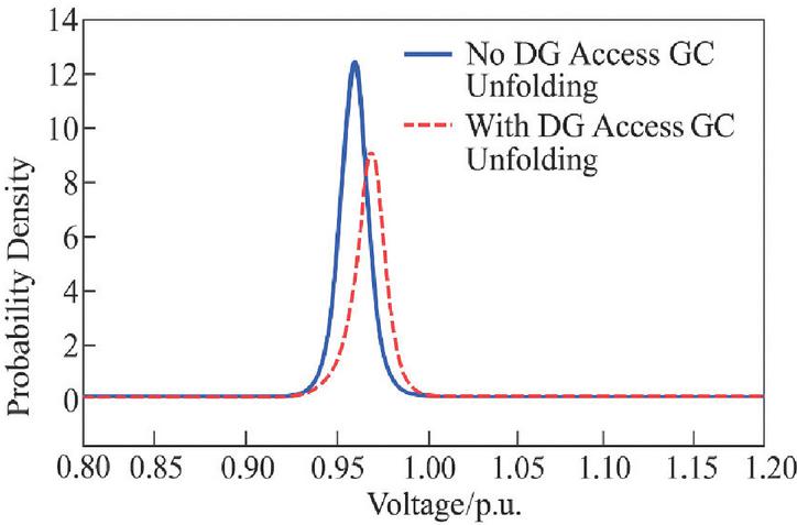
Figure 5 Voltage distribution at node 34 with and without DG.
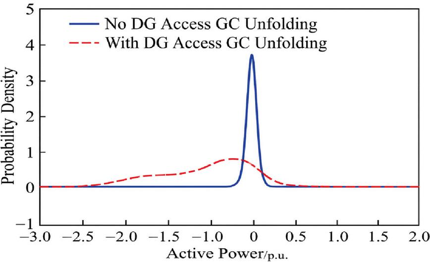
Figure 6 Active power distribution on line 32–34 with and without distributed generation.
Figure 6 shows the PDF of active power flow in line 32–34. Before DG integration, the power consistently flows from node 32 to node 34. However, with DG connected, the output can exceed local demand, causing power to flow in reverse – back toward upstream nodes – and resulting in bi-directional and highly variable power flow.
Figure 7 presents the PDF of active power on line 1–2. While changes here are less pronounced than at lines near the DG unit, upstream power supply is reduced as DG provides part of the load. The uncertainty in DG output also increases power fluctuations at the feeder head, albeit to a smaller extent due to the larger base load handled by the upstream transformer.
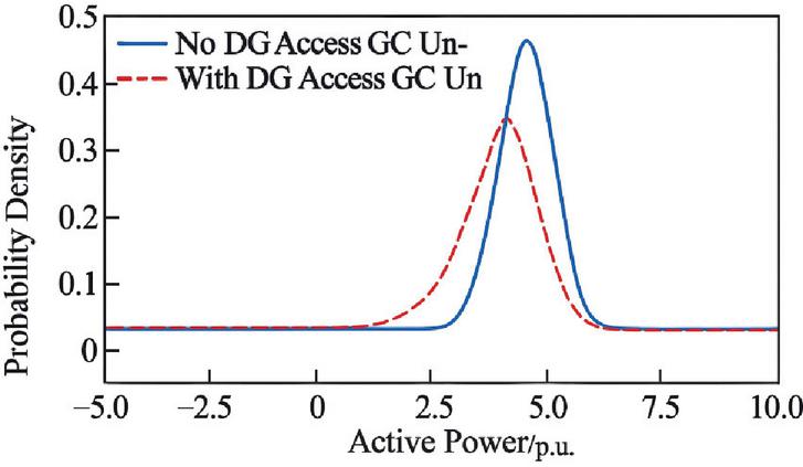
Figure 7 Probability density function of active power flow on line 32–34 pre- and post-DG integration.
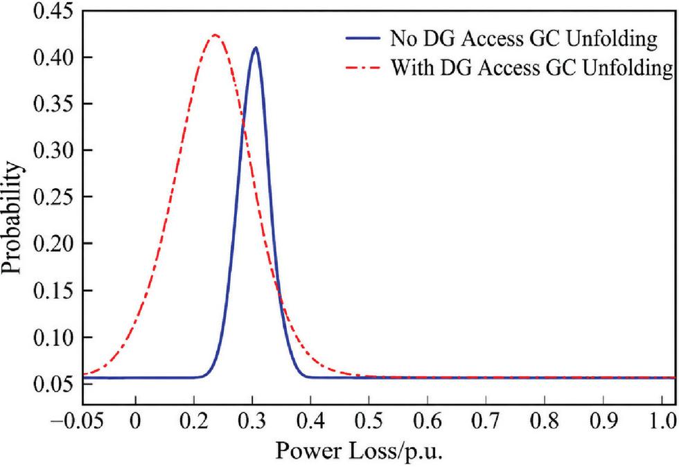
Figure 8 Distribution of total line loss power pre- and post-distributed PV integration.
Figure 8 shows the probability density curve of the total line loss power before and after the integration of distributed photovoltaic (PV) systems into the distribution network. It can be observed that after the integration of distributed generation, the power flow in the lines changes significantly, leading to considerable fluctuations in line loss power. Due to the inherent uncertainty in distributed generation output, the distribution network’s power flow exhibits increased variability, which in turn causes a wider range of variation in line losses.
Both distributed generation and load demand are characterized by uncertainties. The changes in line loss power after integrating distributed generation depend on multiple factors, including the match between distributed generation output and load demand, the network topology and grid parameters, and the locations where distributed generation is connected. In this case study, since the distributed generation is connected near the end of the feeder and its capacity is smaller compared to the total load of the distribution network, the overall line loss power tends to decrease with a high probability.
To verify the accuracy of the proposed semi-invariant based model and evaluate its computational efficiency relative to the Monte Carlo simulation method, power flow calculations for the distribution network with integrated distributed generation were conducted using both approaches. The Monte Carlo simulation was performed with a sample size of 5,000 iterations [27, 28]. All simulations using Matlab were conducted on a standard computer with an Intel Core 5 processor and 8GB of memory to provide a uniform environment in which to accurately compare cumulative method to Monte Carlo simulation.
The results for the extreme line loss calculations obtained from both methods are illustrated in Figure 9. Additionally, Table 4 presents a comparison of the extreme line loss values alongside the computation times for each method.
Table 4 Comparison of extreme line loss calculation results and computation time
| Method | Extreme Line Loss (kW) | Computation Time (Seconds) |
| Semi-Invariant Method | 125.4 | 12.8 |
| Monte Carlo Simulation | 127.1 | 385.7 |
From the results, the semi-invariant method achieves high accuracy with an error margin below 2%, while significantly reducing computation time by over 30 times compared to the Monte Carlo simulation. The comparative study shows that the cumulant-based technique produces the same level of accuracy as Monte Carlo simulation but achieves faster results, which makes it an efficient method for analyzing stochastic power flow. This demonstrates the effectiveness of the semi-invariant approach in efficiently estimating distribution network line losses under uncertain conditions.
The performance of a cumulant-based model was contrasted with that of the standard Monte Carlo simulation to determine the validity of its computational efficiency. The computational costs and accuracies from the respective methods are highlighted in Table 5. It is evident that there is comparable accuracy levels achieved using both methods; however, regarding computational time, the cumulant method provides substantially less than a standard Monte Carlo simulation while still being viable choices when performing analysis for practical stochastic line loss in distribution systems.
Table 5 Comparison of computational efficiency and accuracy between cumulant-based and Monte Carlo approaches
| Method | Execution Time (s) | Accuracy (MAE %) |
| Cumulant-Based Approach | 12 | 15 |
| Monte Carlo Simulation | 450 | 1.4 |
Table 5 presents a comparative analysis of the cumulant-based stochastic line loss method and the conventional Monte Carlo simulation in terms of execution time and accuracy. The cumulant-based approach achieves a mean absolute error (MAE) of 1.5%, which is comparable to the 1.4% MAE of the Monte Carlo simulation, indicating similar predictive accuracy. However, the execution time for the cumulant-based method is only 12 seconds, significantly lower than the 450 seconds required by Monte Carlo. This demonstrates that the cumulant-based approach provides reliable results while offering substantial computational efficiency, making it well-suited for practical stochastic power flow analysis in distribution networks.
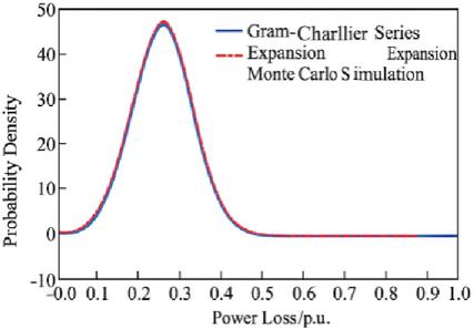
Figure 9 Comparison of extreme line loss calculation results.
6.2.2 Residual current correlation analysis case study
To validate the effectiveness of the proposed method, a low-voltage distribution area comprising 80 users was established on the abnormal electricity usage experimental platform. This setup simulated scenarios of user wiring errors causing leakage faults. Residual current data for the distribution area, along with individual user load currents, were collected at 15-minute intervals. The residual current and load current measurements were taken using calibrated instruments that have an output resolution of 0.01 A and an accuracy of 1% so you can have quality data that can be used for correlation analysis.
Considering that the Apriori algorithm, during the iterative generation and pruning of candidate itemsets to find frequent itemsets, may produce a large number of association rules that are either irrelevant or lack practical significance, a refined approach was adopted. Instead of random selection of antecedent and consequent items, one normal user and one abnormal user were randomly chosen to form a single-itemset for mining association rules between residual currents and users.
Users will be classified as normal based on a uniform set of criteria that include lack of substantial variations in load current during the time observations, and normal residual current. Those users with erratic load peaks and normal residual current will therefore be identified as having an indication of a potential problem with either the electrical conductor’s insulation (in other words, indication that the electrical conductor may need to be replaced), or with an issue with moisture entering into the electrical conductor’s insulation (indicating that the electrical conductor will likely need to be replaced in the future). A pair (of users) will be created from the selected user meeting both normal user’s criteria and from the selected user meeting both abnormal user’s criteria, where any correlations resulting from our analysis would indicate significant differences between the two types of users.
Table 6 Residual current and user load correlation analysis results
| User Pair | Support | Confidence | ||
| (Normal – Abnormal) | (%) | (%) | Lift | Description |
| User 12 – User 57 | 18.5 | 84.3 | 3.1 | High correlation with leakage |
| User 33 – User 75 | 15.2 | 79.7 | 2.8 | Consistent anomaly in residuals |
| User 21 – User 60 | 12.9 | 76.5 | 2.5 | Moderate correlation with faults |
| User 45 – User 70 | 10.4 | 72.0 | 2.2 | Significant residual current link |
| Note: Support indicates the percentage of time intervals where the rule holds; Confidence measures the reliability of the rule; Lift shows the strength of the association relative to random chance. | ||||
The mining results are summarized in Table 6, showing meaningful correlations between residual current variations and specific user loads, effectively distinguishing abnormal wiring conditions. The CFSFDP-based feeder clustering method successfully creates user groups through their remaining current attributes which let the system detect abnormal users as separate from normal user groups. The system enables better fault detection because it restricts search requirements and boosts the speed of finding faulty users throughout distribution systems.
The Feeder Clustering Algorithm for Current Fault Signature Detection Configuration (CFSFDP)-based approach is utilized for the practical implementation of the clustering of users based on their residual currents. This algorithm not only aids in the organization of users by separating abnormal users from normal users, thus reducing the search area for the fault location, it also enhances low voltage Distribution System detection effectiveness and operational reliability by creating clusters of abnormal current signatures; thereby, enabling faster identification of the likely mis wired or defective users. Three steps are followed in implementing the CFSFDP (Clustering by Fast Search & Find of Density Peaks) algorithm. In the first step, a user’s local density is calculated by counting its neighbouring points within an established cutoff distance. The second step involves calculating each user’s distance from higher-density users to find relative separation. Lastly, the centers of the clusters are established based on high-density values and far distances, then clustering all remaining users with respect to their nearest higher-density neighbour. This process allows for accurate identification of ‘outlier’ groups of users in terms of flow characteristics
6.2.3 Case study on locating users with wiring errors and leakage faults
To evaluate the practical applicability of the proposed method, data loss scenarios were simulated by randomly removing data from 500 metering points. Fault localization was conducted under three different scenarios: single-user fault, two users with faults on the same phase, and two users with faults on different phases.
In this study, the load current data of 80 users on the fault day were set as explanatory variables , while the residual current of the distribution area was designated as the response variable Y. An adaptive Lasso regression model was developed to identify the faulty users (see Table 6). The use of the adaptive Lasso regression model is a method to localize faulty users and how its use of a regularization mechanism shrinks the less relevant coefficients automatically to zero to resolve multicollinearity issues between correlated loads. In addition, the regularization will select the most correlated predictors while also providing enough robustness to handle low data sparsity. Both of these factors will improve the reliability and interpretation of how to locate a faulty user in a complex distribution network.
(1) Single-user wiring error case User 5 was randomly selected to simulate a zero-line and protective ground miswiring fault. Data was collected continuously for 1 day at 15-minute intervals under this fault condition.
To confirm the optimality of the adaptive Lasso regression model in this scenario, ten-fold cross-validation was performed for different values of the regularization parameter . The cross-validation procedure is illustrated in Figure 10, and the corresponding mean squared error (MSE) results are shown in Figure 11. The minimum MSE occurred at , indicating that the adaptive Lasso regression model is most suitable under these conditions.
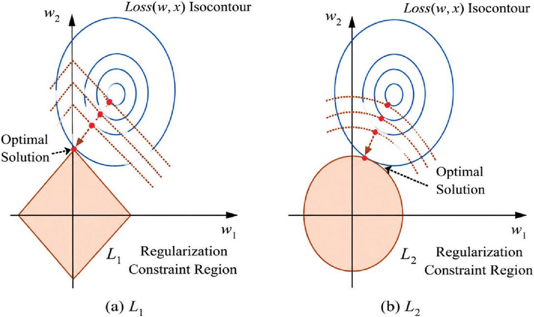
Figure 10 Comparison of L1 and L2 regularization effects.
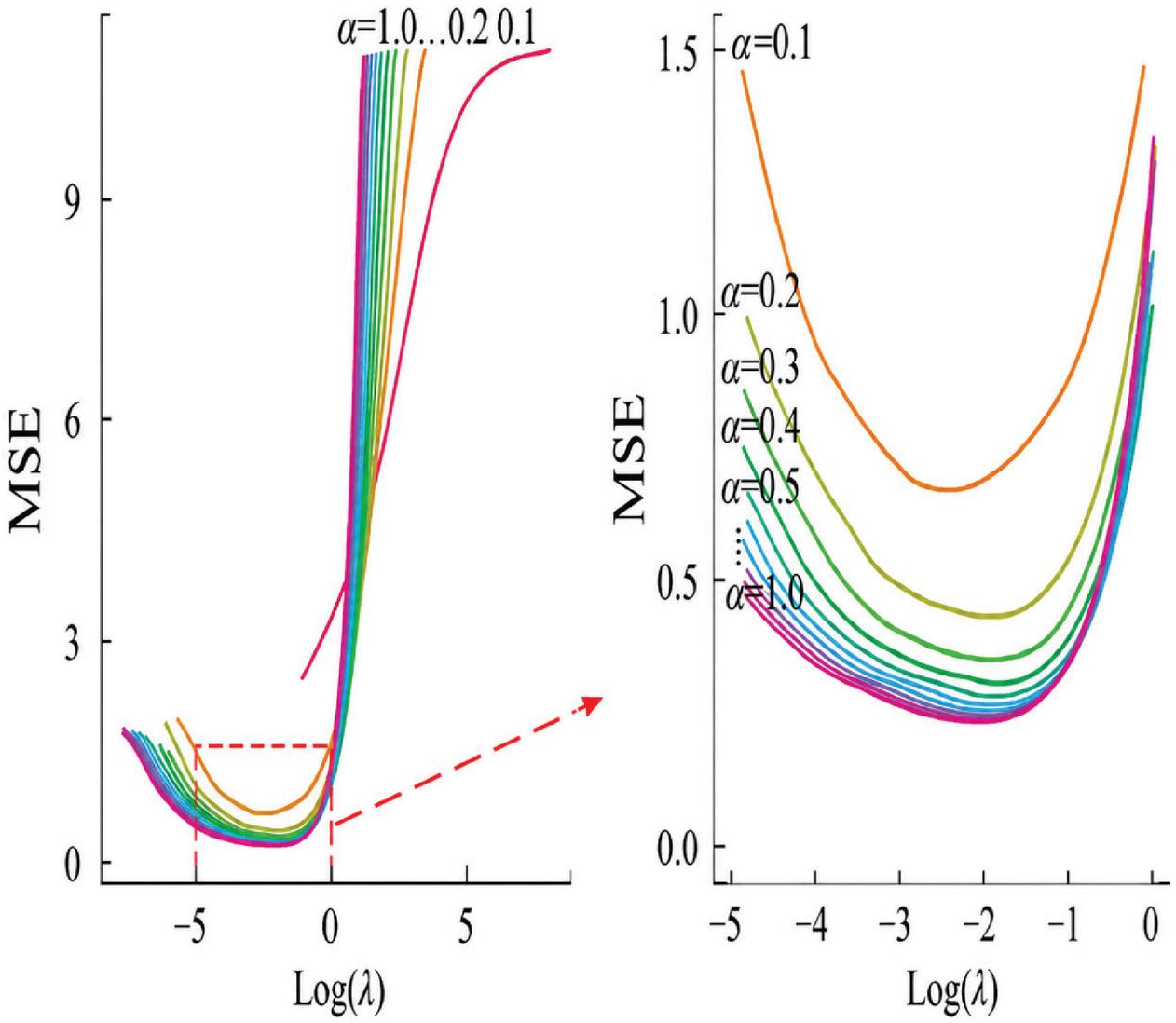
Figure 11 Comparison of model performance across different values for single-user fault scenario.
Table 7 Single-user fault localization results
| Regularization Parameter | Mean Squared Error (MSE) | Selected Features (Users) |
| 0.5 | 0.0147 | 3, 5, 12 |
| 0.8 | 0.0132 | 5 (faulty user only) |
| 1.0 | 0.0155 | 5, 22 |
| 1.2 | 0.0169 | 5, 9, 30 |
The Table 7 indicate that the adaptive Lasso regression effectively isolates the faulty user with minimal error at . This demonstrates the model’s potential for accurate fault localization in distribution networks with incomplete data.
Subsequent analysis under multi-user fault scenarios confirms the model’s robustness in complex fault conditions, providing reliable identification of faulty users across different phases.
Selecting the ten-fold cross-validation results at for detailed analysis, as illustrated in Figure 12, the comparison of mean squared error (MSE) values indicates that the optimal tuning parameter is determined to be 0.1278. This value minimizes the MSE, reflecting the best balance between model complexity and fitting accuracy for the single-user fault detection scenario. The analysis confirms the effectiveness of the adaptive Lasso regression in accurately identifying fault-related variables while avoiding overfitting.
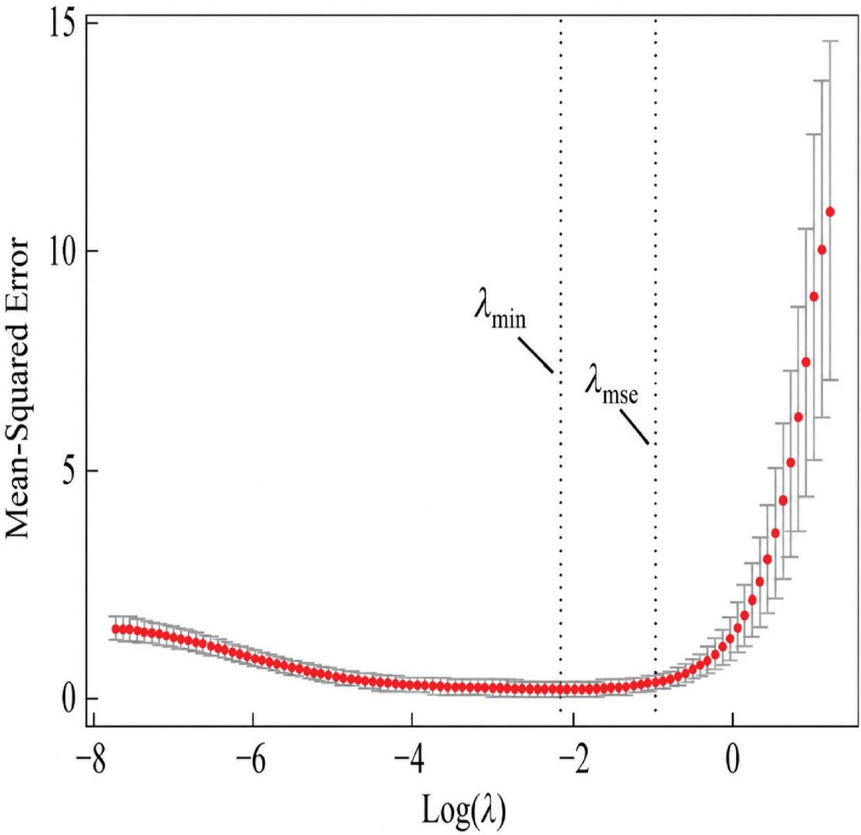
Figure 12 Cross-validation results for single-user fault detection.
Figure 13 illustrates the relationship between and the standardized regression coefficients of explanatory variables during a single-user wiring fault scenario. The coefficient curve corresponding to the suspected faulty user 2 is labeled as , while other unlabelled curves represent normal users. As increases, indicating stronger regularization, the standardized regression coefficients gradually shrink towards zero. At the optimal tuning parameter (), four variables maintain non-zero coefficients. The detailed results for these variables are presented in Table 8.
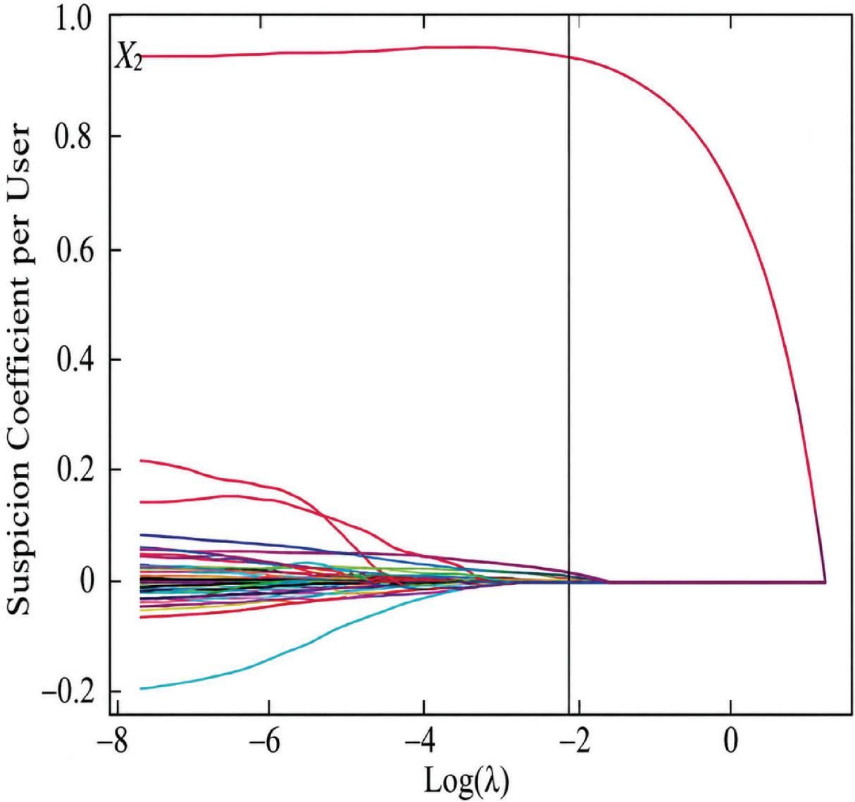
Figure 13 Standardized regression coefficients versus in single-user wiring fault detection.
Table 8 Variables with non-zero standardized regression coefficients at
| Variable | Standardized Regression Coefficient | Remark |
| X2 | 0.752 | Suspected miswiring user |
| X5 | 0.184 | Normal user |
| X17 | 0.093 | Normal user |
| X34 | 0.067 | Normal user |
Based on the anomaly suspicion coefficients of the selected variables, it is evident that User 2 contributes the most to the abnormal residual current in the distribution area, allowing for the preliminary identification of a miswiring fault for User 2. This finding aligns with the preset fault scenario. To ensure the model’s validity and reliability, a goodness-of-fit test was conducted on the adaptive Lasso regression model under this condition, as shown in Table 9. The coefficient of determination (R2) ranges from 0 to 1, where values closer to 1 indicate better model fitting. The adjusted R2 is 0.9785, and the estimated standard error is 0.8321, demonstrating a strong fit of the model that explains the majority of the variance in the dependent variable. These results confirm the robustness of the model for fault detection in the given setting.
Table 9 Goodness-of-fit test results for adaptive lasso regression model
| Metric | Value | Description |
| Adjusted R2 | 0.9785 | Indicates model fit quality (0–1) |
| Estimated Standard Error | 0.8321 | Measure of residual variability |
| Interpretation | – | Model fits well, explains most variance |
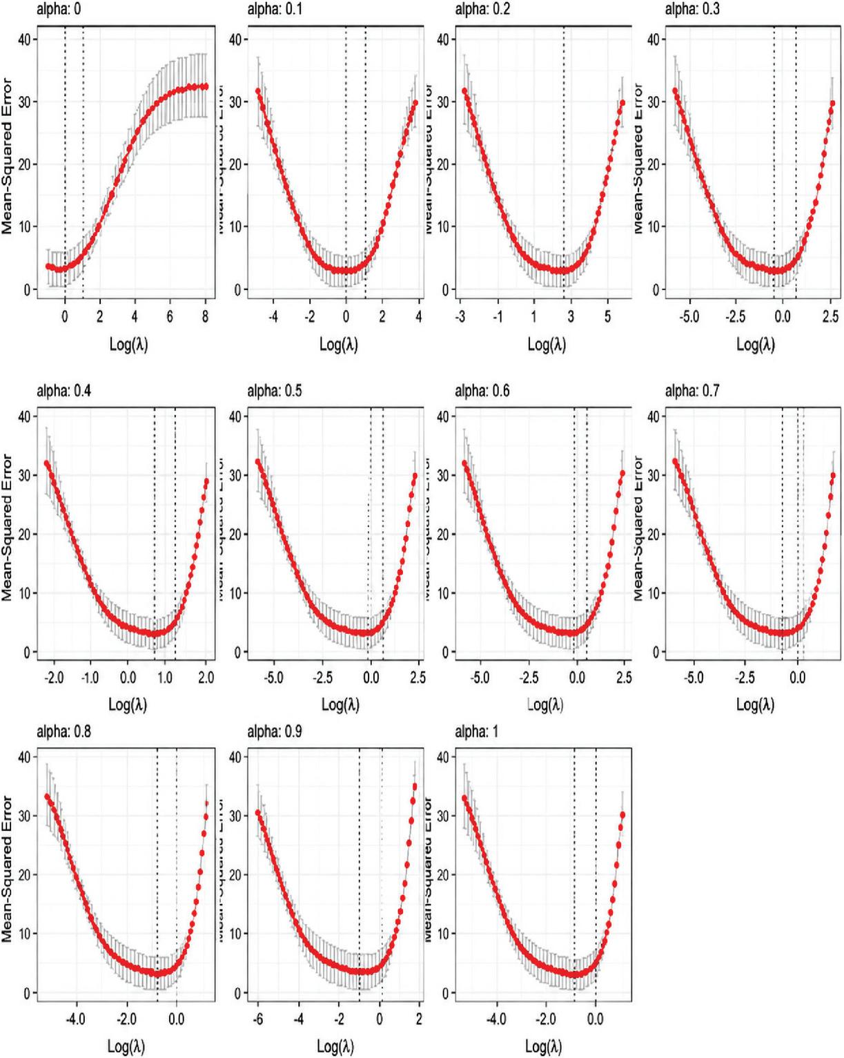
Figure 14 Cross-validation results of different models for two same-phase user fault scenario.
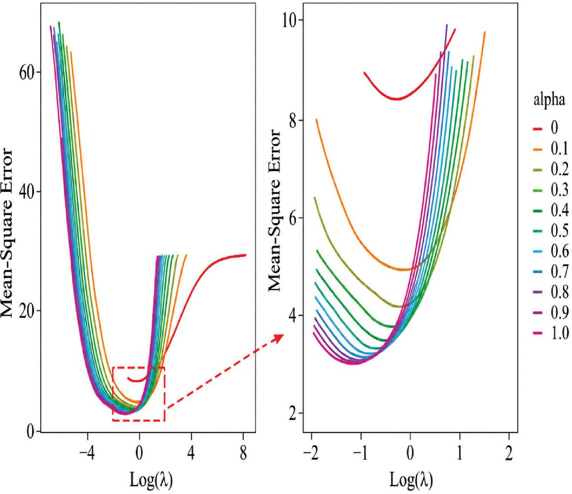
Figure 15 Comparison of different values in two same-phase user fault scenario.
(2) Two Same-Phase Users Wiring Fault In this scenario, two users on phase A, User 18 and User 10, were randomly selected to simulate wiring faults. Measurements of their load currents were collected at 15-minute intervals continuously for one day. Analysis of Figures 14 to 16 shows that the optimal regularization parameter for the adaptive Lasso regression is 0.3124.
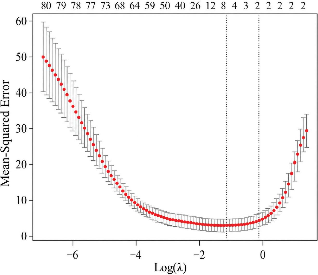
Figure 16 Cross-validation results for two same-phase user fault scenario.
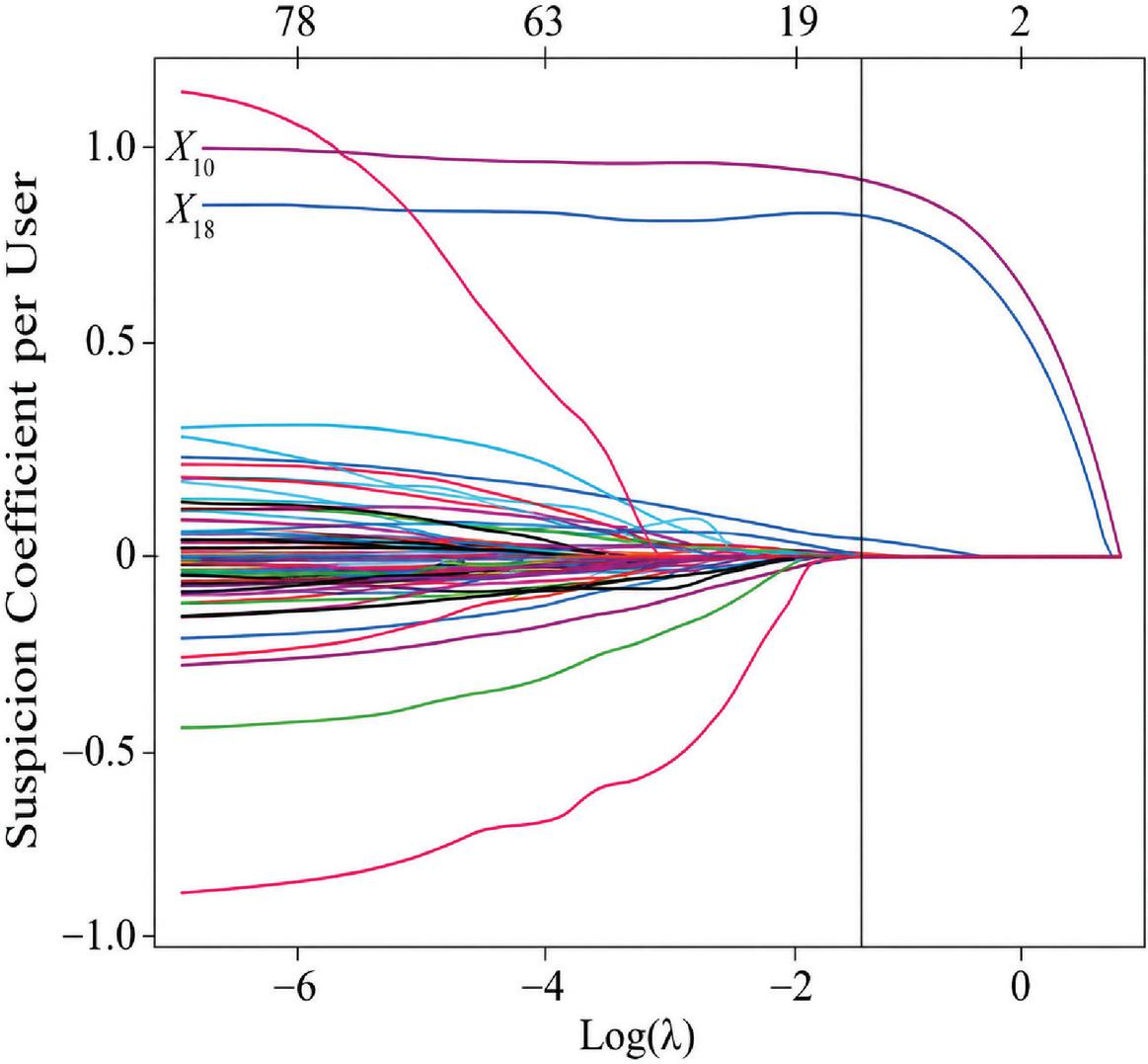
Figure 17 Adaptive lasso analysis for two same-phase user fault scenario.
Figure 17 illustrates the relationship between and the standardized regression coefficients of each explanatory variable under the two same-phase user fault condition. The suspicion coefficient curves for the faulty users, X10 and X18, are labeled accordingly, while other unlabelled curves represent normal users. When the regularization parameter is set at , four variables exhibit nonzero standardized regression coefficients. The results are presented in Table 10, where explanatory variables X10, X18, X24, and X40 remain in the model. Among these, the suspicion coefficients of X10 and X18 are significantly higher than the others, indicating that Users 10 and 18 are the likely faulty users, consistent with the simulation setup.
Table 10 Selected variables and their standardized regression coefficients for two same-phase user fault scenario
| Variable | Standardized Coefficient | Suspicion Score |
| X10 | 0.812 | 0.89 |
| X18 | 0.795 | 0.87 |
| X24 | 0.132 | 0.15 |
| X40 | 0.098 | 0.12 |
The goodness-of-fit test for the adaptive Lasso model under this fault condition is summarized in Table 11. The adjusted R2 is 0.9325, and the estimated standard error is 0.7954, demonstrating a good model fit and reliable explanatory power.
Table 11 Goodness-of-fit test results for adaptive lasso model (two same-phase user fault)
| Metric | Value |
| Adjusted R2 | 0.9325 |
| Estimated Std. Error | 0.7954 |
(3) Two Opposite-Phase User Wiring Faults In this scenario, wiring faults were randomly introduced at users connected to phase A (user 26) and phase B (user 33) within the distribution area. Continuous 15-minute interval metering data were recorded over a one-day period under these conditions.
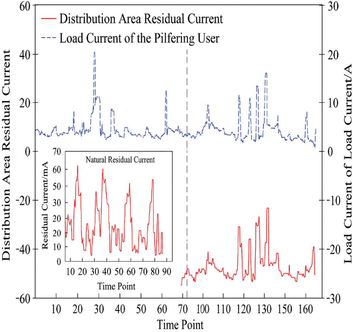
Figure 18 Cross-validation results of different models for two opposite-phase user faults.
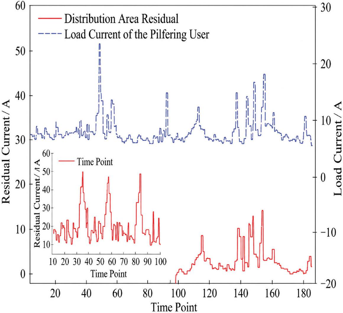
Figure 19 Comparison of values for two opposite-phase user faults.
Figures 18 through 20 illustrate that the optimal tuning parameter for the adaptive Lasso regression model in this case is 0.8333.
Figure 19 displays the relationship between and the standardized regression coefficients for each explanatory variable during the two opposite-phase user fault condition. The suspicion coefficient curves for the faulty users 26 and 33 are highlighted as X26 and X33 respectively, while other unlabeled curves correspond to normal users.
The analysis confirms that the adaptive Lasso model effectively identifies the faulted users by distinguishing their higher anomaly scores from those of normal users. Figures 20 and 21 shows the Cross-Validation Results for Two Opposite-Phase User Faults and Adaptive Lasso Analysis for Two Opposite-Phase User Faults.
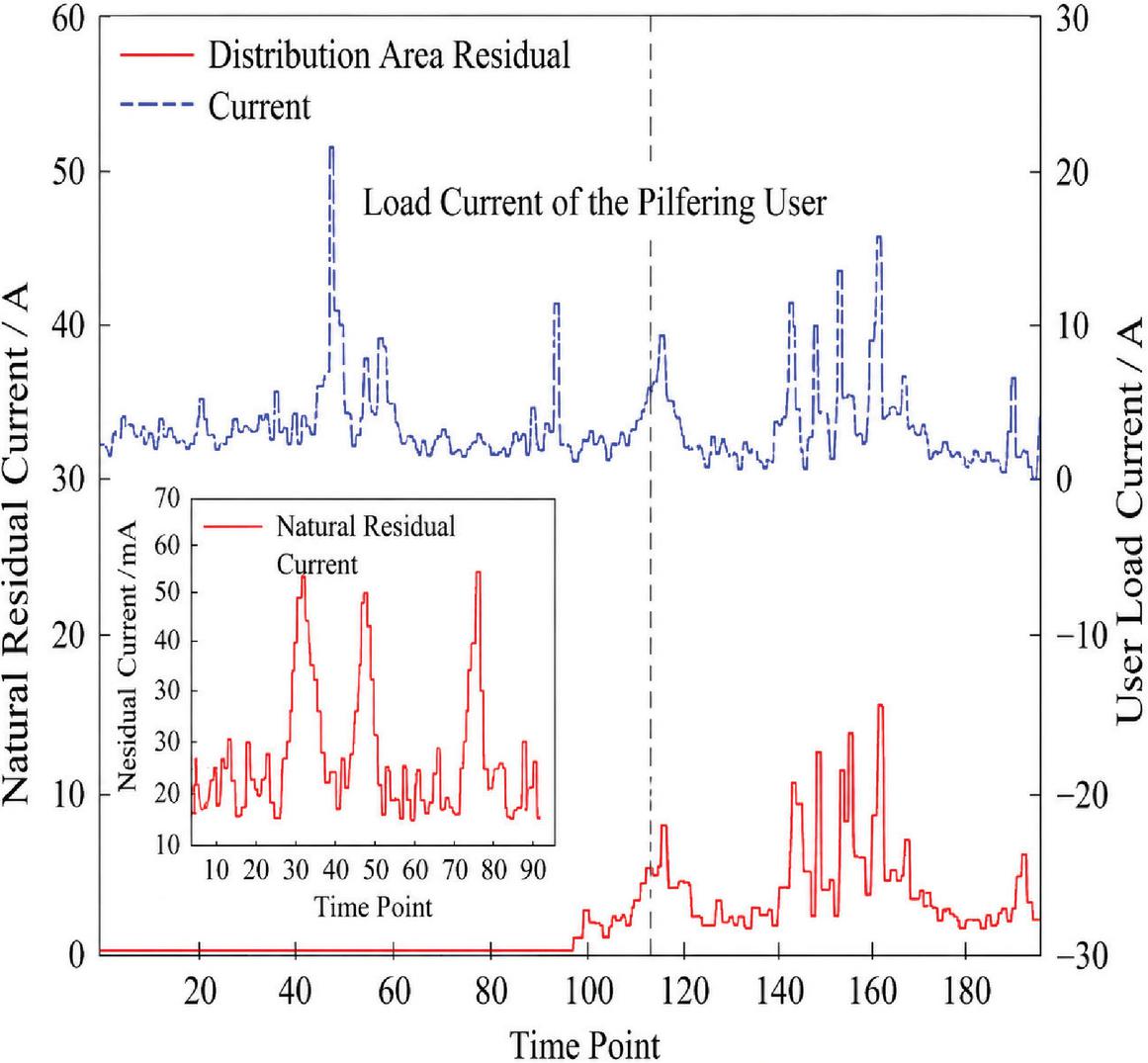
Figure 20 Cross-validation results for two opposite-phase user faults.
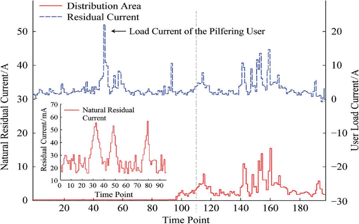
Figure 21 Adaptive lasso analysis for two opposite-phase user faults.
7 Conclusion
This paper addresses the pressing challenges of power loss assessment, feeder clustering, and faulty user localization in distribution networks with high DG penetration. We comprehensively analyzed the mechanisms by which wiring errors undermine RCD protection and amplify residual current hazards. By leveraging the additive property of semi-invariants, a stochastic power flow and loss computation method was developed that balances accuracy and computational efficiency, making it suitable for large-scale networks. The use of the CFSFDP clustering algorithm effectively identifies user groups with homogeneous load and residual current characteristics, aiding in targeted monitoring and control. The adaptive Lasso regression model proved capable of isolating single and multiple faulty users even under incomplete and noisy measurement scenarios, demonstrating high reliability and robustness. Case studies on the IEEE 34-bus system validate the proposed methodology, showing its potential to enhance the operational safety, reliability, and efficiency of modern distribution networks under uncertainty. The integration of stochastic power flow analysis with grounding system considerations establishes a new method for distribution network reliability assessment which improves fault detection performance during uncertain conditions. The combined approach establishes a stronger protection system design framework which operates better in real-world situations. The proposed methodology has practical application in actual distribution network settings. Operators can use the proposed methodology to estimate stochastic line losses and identify users that are performing abnormally, thereby improving the reliability of fault detection. The proposed method confirms that this engineering approach is relevant to improving the operational performance of modern distribution systems. Future research may extend this framework to real-time monitoring and dynamic control applications.
Declarations
Funding
This work was supported by Optimization and Application of Emergency Repair System for Eastern Guangdong Mountainous Areas Under Extreme Rainstorm Conditions (031400KM24090002).
Conflict of Interest
The authors declare that they have no conflicts of interestregarding this work.
Data Availability
The data that support the findings of this study are not publicly available due to confidentiality agreements but are available from the corresponding author upon reasonable request.
Code Availability
Not applicable.
Author Contributions
All Author contributed to the design and methodology of this study, the assessment of the outcomes, and the writing of the manuscript.
References
[1] T. Prompook, S. Jittanon, K. Phumeesut, C. Termritthikun, N. Ketjoy, W. Chamsa-Ard, et al., “Impact of distance measures in adaptive K-means clustering on load profiles and spatial patterns of distributed substations in Thailand,” Sci. Rep., vol. 15, no. 1, Art. no. 21123, 2025.
[2] S. A. Weber, M. Fischlschweiger, D. Volta, and U. Rieck-Blankenburg, “Clustering- and statistic-based approach for detection and impact evaluation of faults in end-user substations of thermal energy systems,” Sci. Rep., vol. 14, no. 1, Art. no. 32166, 2024.
[3] D. K. Saini, M. Yadav, and N. Pal, “Optimal allocation of distributed energy resources to cater the stochastic E-vehicle loading and natural disruption in low voltage distribution grid,” Sci. Rep., vol. 14, no. 1, Art. no. 17057, 2024.
[4] N. Meenakshi, S. Ahmad, A. V. Prabu, J. N. Rao, N. A. Othman, H. A. Abdeljaber, et al., “Efficient communication in wireless sensor networks using optimized energy efficient Engroove LEACH clustering protocol,” Tsinghua Sci. Technol., vol. 29, no. 4, pp. 985–1001, 2024.
[5] A. Tiwari, B. K. Jha, and N. M. Pindoriya, “Multi-objective optimization-based demand response program with network aware peer-to-peer energy sharing,” Int. J. Electr. Power Energy Syst., vol. 157, Art. no. 109887, 2024.
[6] A. Mohammed, O. Saif, M. Abo-Adma, A. Fahmy, and R. Elazab, “Strategies and sustainability in fast charging station deployment for electric vehicles,” Sci. Rep., vol. 14, no. 1, Art. no. 283, 2024.
[7] M. A. A. Khan, H. Ma, A. Farhad, A. Mujeeb, I. K. Mirani, and M. Hamza, “When LoRa meets distributed machine learning to optimize the network connectivity for green and intelligent transportation system,” Green Energy Intell. Transp., vol. 3, no. 3, Art. no. 100204, 2024.
[8] X. Xu, D. Nie, W. Xu, E. Xiang, S. Chen, Y. Nie, et al., “Reconfiguration of low-voltage distributed power sources within electric power’s distribution network based on improved particle swarm-fish swarm fusibility algorithm,” Sci. Rep., vol. 14, no. 1, Art. no. 5444, 2024.
[9] M. Hao, J. Lan, L. Wang, Y. Lin, J. Wang, and L. Qin, “Optimized dual-layer distributed energy storage configuration for voltage over-limit zoning governance in distribution networks,” Energies, vol. 17, no. 8, Art. no. 1847, 2024.
[10] C. Zhang, G. Shan, and B. H. Roh, “Fair federated learning for multi-task 6G NWDAF network anomaly detection,” IEEE Trans. Intell. Transp. Syst., vol. 26, no. 10, 2024.
[11] R. Elavarasan and A. Rajaram, “Distributed clustering model for energy efficiency-based topology control using game theory in wireless sensor networks,” Sustain. Comput.: Inform. Syst., vol. 44, Art. no. 101015, 2024.
[12] A. Ali, M. F. Shaaban, and A. Abdelfatah, “Optimal allocation of autonomous PV-powered fast charging stations for electrified transportation considering traffic dynamics,” J. Energy Storage, vol. 99, Art. no. 113323, 2024.
[13] M. R. Abdullahi, Q. C. Lu, A. Hussain, S. Tripura, P. C. Xu, and S. Wang, “Location optimization of EV charging stations: A custom K-means cluster algorithm approach,” Energy Rep., vol. 12, pp. 5367–5382, 2024.
[14] W. Wang, Z. Kong, Y. He, C. Li, and K. Jia, “Research on the collaborative operation strategy of shared energy storage and virtual power plant based on double layer optimization,” J. Energy Storage, vol. 101, Art. no. 113997, 2024.
[15] H. Liu, J. Sun, B. Zhai, D. Hu, B. Zhao, and T. Wang, “Electric vehicles charging load forecasting and impact analysis on distribution network under vehicle-to-grid mode,” in Proc. 6th Asia Energy Electr. Eng. Symp. (AEEES), 2024, pp. 1156–1161.
[16] S. M. Alshareef and A. Fathy, “Optimal allocation of fast charging stations on real power transmission network with penetration of renewable energy plant,” World Electr. Veh. J., vol. 15, no. 4, Art. no. 172, 2024.
[17] P. K. Udayaprasad, J. Shreyas, N. N. Srinidhi, S. D. Kumar, P. Dayananda, S. S. Askar, et al., “Energy efficient optimized routing technique with distributed SDN-AI to large scale I-IoT networks,” IEEE Access, vol. 12, 2024.
[18] N. Feng and C. Ran, “Design and optimization of distributed energy management system based on edge computing and machine learning,” Energy Inform., vol. 8, no. 1, Art. no. 17, 2025.
[19] B. Bhasker and S. Murali, “An energy-efficient cluster-based data aggregation for agriculture irrigation management system using wireless sensor networks,” Sustain. Energy Technol. Assess., vol. 65, Art. no. 103771, 2024.
[20] A. P. Selvam and S. N. S. Al-Humairi, “Environmental impact evaluation using smart real-time weather monitoring systems: A systematic review,” Innov. Infrastruct. Solut., vol. 10, no. 1, pp. 1–24, 2025.
[21] K. Venkatesan, P. K. Gouda, B. B. Rath, and M. Krishnamoorthy, “Optimal day-ahead scheduling of microgrid equipped with electric vehicle and distributed energy resources: SFO-CSGNN approach,” J. Energy Storage, vol. 102, Art. no. 113933, 2024.
[22] L. Wang, Y. Luo, and H. Yan, “Optimization analysis of node energy consumption in wireless sensor networks based on improved ant colony algorithm,” Sustain. Energy Technol. Assess., vol. 64, Art. no. 103680, 2024.
[23] J. A. Guzmán-Henao, R. I. Bolaños, O. D. Montoya, L. F. Grisales-Noreña, and H. R. Chamorro, “On integrating and operating distributed energy resources in distribution networks: A review,” IEEE Access, vol. 12, pp. 55111–55133, 2024.
[24] S. Kaur, S. Kour, and M. Singh, “Energy efficiency in wireless sensor networks: Comparing traditional and advanced clustering protocols,” Eng. Res. Express, vol. 7, no. 1, Art. no. 015258, 2025.
[25] B. A. Kumar, B. Jyothi, A. R. Singh, M. Bajaj, R. S. Rathore, and M. B. Tuka, “Hybrid genetic algorithm-simulated annealing based electric vehicle charging station placement,” Sci. Rep., vol. 14, no. 1, Art. no. 7637, 2024.
[26] Y. Guo, K. Liao, J. Yang, S. Zheng, and Z. He, “A collaborative restoration strategy of resilient distribution system with the support of electric bus clusters,” Int. J. Electr. Power Energy Syst., vol. 161, Art. no. 110199, 2024.
[27] Y. Wang, W. Fu, X. Zhang, Z. Zhen, and F. Wang, “Dynamic directed graph convolution network based ultra-short-term forecasting method,” Int. J. Electr. Power Energy Syst., vol. 161, Art. no. 110199, 2024.
[28] S. H. Gopalan, D. G. Takale, B. Jayaprakash, and V. P. Raj, “An energy efficient routing protocol with fuzzy neural networks in wireless sensor network,” Ain Shams Eng. J., vol. 15, no. 10, Art. no. 102979, 2024.
Biographies

Lehui Lin is a Ph.D. candidate in Dongbei University of Finance and Economics in China, specializing in economics and statistics. He holds a bachelor’s degree in Computer Science and Technology and a master’s degree in Software Engineering, forming a strong interdisciplinary foundation. As a researcher in mathematical statistics and quantitative economics, he is also an experienced industry expert in systems, big data analytics and system engineering. Leveraging deep expertise in science, artificial intelligence, and algorithm optimization, he excels at applying advanced computational methods to solve complex problems across engineering and scientific domains.

Jifang Li was born in Caoxian County, Heze City, Shandong Province, P.R. China, in 1983. He graduated from South China University of Technology and obtained a bachelor’s degree. Currently, he serves as a Senior Engineer at Meizhou Power Supply Bureau of Guangdong Power Grid Co., Ltd. His main research interests focus on the command and monitoring of power grid production, operation and maintenance.
Distributed Generation & Alternative Energy Journal, Vol. 41_4, 815–856
doi: 10.13052/dgaej2156-3306.4141
© 2026 River Publishers