MPC-Guided Deep Reinforcement Learning for Real-Time Scheduling of Microgrid with Uncertainty

Yilu Zhang^* and Xiaobing Kong

North China Electric Power University, Beijing, China
E-mail: zhangzhang00777@163.com
*Corresponding Author

Received 26 February 2026; Accepted 24 March 2026

Abstract

Microgrid energy management plays a critical role in ensuring the secure and economical operation of microgrids. To address the uncertainty of renewable energy generation, this paper proposes an MPC-guided deep reinforcement learning (DRL)–based intraday scheduling strategy for microgrids. The proposed approach integrates the advantages of model predictive control (MPC) and DRL, where the optimization results of the MPC module are provided as environmental inputs to the DRL agent, and the DRL module interacts with the real microgrid environment to generate compensation actions. This framework not only mitigates the performance degradation caused by uncertainties in model-based methods, but also reduces the search space of DRL, thereby accelerating training convergence and suppressing policy fluctuations. Comparative simulations are conducted against standalone MPC and standalone DRL controllers. The results demonstrate that the proposed strategy can significantly reduce both operational security cost and economic cost, while effectively improving the utilization of renewable energy. Therefore, it provides an innovative solution for the microgrid scheduling problem.

Keywords: Microgrid, real-time scheduling, model predictive control, deep reinforcement learning, deep deterministic policy gradient.

1 Introduction

With the continuous growth of global energy demand, the traditional fossil-fuel–dominated energy structure has led to increasingly prominent resource constraints and environmental problems. Driven by the global transition toward low-carbon and sustainable energy systems, renewable energy sources, such as solar and wind power, are gradually becoming an important alternative to conventional fossil-fuel-based power generation due to their clean and sustainable characteristics. In recent years, rapid technological progress and the continuous expansion of installed capacity have further strengthened the role of renewable energy in the global energy system. In 2025, Science magazine listed the rapid development of renewable energy among its top scientific breakthroughs of the year, highlighting its critical role in promoting energy transition and sustainable development [1].

Microgrids, as an important form of integrating Distributed Renewable Energy Sources (DREs), are typically composed of wind power, photovoltaic generation, diesel generators, and energy storage systems. It enables coordinated operation and flexible scheduling of energy resources within a localized area. Through appropriate energy management strategies, microgrids can not only improve the reliability of power supply and power quality, but also enhance the utilization of renewable energy while reducing system operating costs and environmental pollution [2]. Therefore, under the background of high penetration of renewable energy, the optimal scheduling of microgrids has become one of the major research topics both domestically and internationally. Essentially, the microgrid optimization problem aims to achieve the optimal allocation and management of internal energy resources through mathematical algorithms and intelligent control strategies, thereby maximizing the economic efficiency and operational reliability of the microgrid. Classical scheduling approaches mainly include Linear Programming (LP), Nonlinear Programming (NLP), and intelligent optimization algorithms [3, 4].

Traditional optimization techniques exhibit limitations when dealing with high-dimensional, complex, uncertain, and nonlinear microgrid scheduling problems. Consequently, learning-based optimization methods have attracted increasing attention in recent years. Deep Reinforcement Learning, which integrates the advantages of deep learning and reinforcement learning, is capable of effectively handling high-dimensional, nonlinear, and complex state–action spaces through deep neural networks. By continuously interacting with the environment, the DRL agent can autonomously learn optimal strategies based on reward signals, thereby maximizing long-term returns and providing a new technical approach for microgrid optimal scheduling.

Several studies have explored the application of DRL to microgrid energy management. Reference [5] developed a two-layer microgrid scheduling framework based on Deep Q-learning (DQN). Reference [6] proposed a dual-objective value network method based on the clipped double Q-learning concept to achieve real-time energy scheduling for grid-connected microgrids, where system operation strategies are optimized online through reinforcement learning. However, these methods belong to value-based reinforcement learning algorithms, in which the control variables are restricted to discrete actions. In contrast, many control variables in microgrids, such as power allocation, voltage regulation, and charging or discharging commands of energy storage systems, are inherently continuous. Therefore, policy-based algorithms have been introduced for microgrid scheduling, as they are more suitable for continuous control problems. Reference [7] proposed an energy management optimization method for a wind–solar–diesel–battery microgrid by combining stochastic programming with the Proximal Policy Optimization (PPO) algorithm. Reference [8] developed an improved multi-agent twin delayed deep deterministic policy gradient method, in which a Q-network integrating transaction results is employed to enhance the learning performance of agents without sharing policy information.

The above studies are primarily based on single-agent reinforcement learning frameworks. However, in microgrids containing multiple types of controllable devices, the overall scheduling performance is strongly influenced by the coupling relationships among different units. To address this issue, multi-agent reinforcement learning methods have been introduced. Reference [9] proposed a multi-agent deep reinforcement learning framework for energy management in multi-energy grid-connected microgrids, where distributed learning is adopted to minimize system operating costs while achieving coordinated energy optimization. Reference [10] presented a multi-agent-based bi-level active and reactive power coordinated optimization approach, enabling coordinated scheduling of active and reactive power in islanded microgrids to ensure system security and stability while improving economic performance.

Despite these advances, several challenges remain when applying DRL to microgrid scheduling. First, DRL training requires a large amount of interaction data, leading to relatively low learning efficiency. Second, the exploration process during the early training stage may generate unsafe control actions, which is undesirable for power systems with high reliability requirements. In addition, the training process of DRL may suffer from instability or convergence difficulties due to reward design and environmental uncertainties.

Model Predictive Control is a classical optimization method widely used in industrial process control. By relying on predictive models, rolling optimization, and feedback correction mechanisms, MPC can generate stable control strategies while satisfying system constraints [11]. In recent years, MPC has been increasingly applied to microgrid scheduling problems. Reference [12] proposed an enhanced hierarchical MPC strategy that achieves robust dynamic scheduling of integrated energy microgrids under multiple uncertainties through hierarchical coordination and rolling optimization. Reference [13] developed a hybrid economic MPC framework based on time-scale decomposition for microgrid scheduling. Introducing MPC as a guiding strategy for DRL can effectively alleviate the instability and exploration risks associated with DRL training. Existing studies have verified the feasibility of this framework in various domains. For example, Reference [14] applied the MPC-guided DRL framework to optimal charging control of lithium-ion batteries under uncertain environments, while Reference [15] employed it for real-time traffic flow regulation on highways. These studies demonstrate that MPC-guided DRL strategies exhibit significant advantages in systems characterized by high complexity, strong constraints, and dynamic operating conditions.

In this paper, an MPC-guided DRL strategy is developed for a wind–solar–diesel–battery microgrid system. The MPC module performs rolling optimization based on the system mathematical model to generate baseline scheduling commands. The DRL module then interacts with the real environment on this basis and outputs compensation power actions. Simulation results demonstrate that the proposed method achieves lower operational and economic costs while significantly improving renewable energy utilization.

2 Mathematical Model of Microgrid Optimal Dispatch

2.1 Structure of a Typical Microgrid

A microgrid is capable of operating in both islanded mode, where it functions independently of the main grid, and grid-connected mode, where it is synchronized with the utility grid. This paper focuses on a microgrid operating in a grid-connected state, as depicted in Figure 1, which consists of wind turbines (WTs), diesel engines (DEs), photovoltaic systems (PVs), an energy storage system (ESS), the main power grid and load. In this configuration, the PV array is treated as a non-dispatchable unit, while others are treated as dispatchable units. The ESS plays a key role in mitigating the fluctuations caused by renewable energy and managing the power imbalance within the microgrid. By adjusting the discharging or charging power of the battery, the proportion of wind power generation and the power of the diesel engine at each moment, the microgrid achieves economic optimization while meeting user needs. The constraints and costs of each part is introduced in the following text.

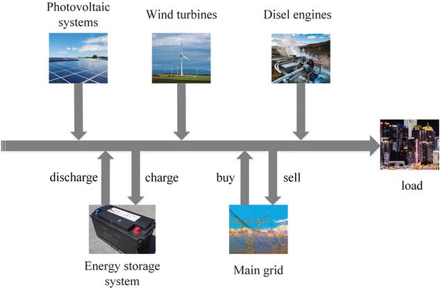
Figure 1 typical microgrid system.

2.2 Microgrid Optimization Problem Formulation

The real-time scheduling of a microgrid aims to adjust the output of distributed energy resources in real time while satisfying system security constraints. The objective is to minimize the deviation between the actual operation and the day-ahead schedule while optimizing operational economy, thereby achieving coordinated optimization between schedule tracking and economic performance:

$$J(t)={\lambda }_{1}C(t)+{\lambda }_{2}E(t)$$

(1)

where $C(t)$ represents the total cost of the microgrid at time $t$, $E(t)$ denotes the tracking deviation of the day-ahead scheduling, and ${\lambda }_1$ and ${\lambda }_2$ are weighting coefficients. Since economic operation is the primary objective of microgrid energy management, a larger weight is assigned to the cost term. Therefore, the weighting coefficients are set as ${\lambda }_1=0.7$ and ${\lambda }_2=0.3$.

The total cost $C(t)$ consists of the economic cost $C_1(t)$ and the security cost $C_2(t)$:

$$C(t)=C_1(t)+C_2(t)$$

(2)

where $C_1(t)=C_{\mathit{wind}}(t)+C_{\mathit{disel}}(t)+C_{\mathit{grid}}(t)$, $C_2(t)=C_{\mathit{exchange}}(t)+C_{\mathit{loss}}(t)$.

The generation cost of the wind turbine $C_{\mathit{wind}}$ is determined by the wind power output $P_{\mathit{wind}}$ and the initial operating cost of the wind turbine $C_{\mathit{initial}}$:

$$C_{\mathit{wind}}(t)=C_{\mathit{initial}}\cdot P_{\mathit{wind}}$$

(3)

The cost of the diesel generator $C_{\mathit{disel}}(t)$ can be expressed as:

$$C_{\mathit{disel}}(t)=a\cdot {(P_{\mathit{diesel}})}^2+b\cdot P_{\mathit{diesel}}+c$$

(4)

where $P_{\mathit{diesel}}$ represents the output power of the diesel generator.

The battery safety cost $C_{\mathit{loss}}(t)$ is given by:

$$C_{\mathit{loss}}(t)={\sigma }_1\ast {(\mathrm{\Delta }{P}_{\mathit{battery}})}^2-{\sigma }_2\ast \mathit{SOC}$$

(5)

where ${\sigma }_1$ and ${\sigma }_2$ denote the safety cost coefficients of the battery, and $\mathrm{\Delta }{P}_{\mathit{battery}}$ represents the variation in the battery charging power.

When energy surplus occurs in the microgrid (e.g., low load demand or high renewable energy output), the excess electricity can be sold to the main grid. Conversely, when the microgrid power supply is insufficient, electricity needs to be purchased from the main grid to meet the load demand. Generally, the selling price is lower than the purchasing price, and both adopt the time-of-use electricity price shown in Figure 2.

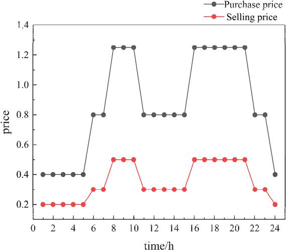
Figure 2 Time-of-Use pricing.

The economic cost of the power exchange between the microgrid and the main grid $C_{\mathit{grid}}(t)$ can be expressed as:

$$C_{\mathit{grid}}(t)=\{\begin{array}{cc}{\mathit{price}}_{\mathit{buy}}\ast P_{\mathit{grid}}\hfill & P_{\mathit{grid}}>0\hfill \\ {\mathit{price}}_{\mathit{sell}}\ast P_{\mathit{grid}}\hfill & P_{\mathit{grid}}<0\hfill \end{array}$$

(6)

where $P_{\mathit{grid}}>0$ indicates that electricity is purchased from the main grid, while $P_{\mathit{grid}}<0$ indicates that electricity is sold to the main grid. $C_{\mathit{grid}}$ represents the economic cost of the power transaction between the microgrid and the main grid.

To balance the economic performance and security of microgrid operation, the security cost associated with power exchange with the main grid is expressed as:

$$C_{\mathit{gridexchange}}(t)=\kappa \ast {(\mathrm{\Delta }{P}_{\mathit{grid}})}^2$$

(7)

where $\kappa$ denotes the cost coefficient of the grid security index.

Since photovoltaic power generation is almost zero during nighttime and its fluctuation is relatively small, the predicted photovoltaic power $P_{\mathit{solar}}^{\mathit{pred}}$ is directly regarded as the actual available power during modeling and simulation. Therefore, the photovoltaic cost is ignored.

The tracking deviation objective of the microgrid from the day-ahead scheduling $E(t)$ is defined as:

$E(t)$	$={\displaystyle \sum _{t=0}^T}{(P_{\mathit{wind}}(t)-P_{\mathit{wind}}^{\text{day–ahead}}(t))}^2+{(\mathit{SOC}(t)-{\mathit{SOC}}^{\text{day–ahead}}(t))}^2$
	$+{(P_{\mathit{disel}}(t)-P_{\mathit{diesel}}^{\text{day–ahead}}(t))}^2$	(8)

where $P_{\mathit{wind}}^{\text{day–ahead}}(t),{\mathit{SOC}}^{\text{day–ahead}}(t),P_{\mathit{diesel}}^{\text{day–ahead}}(t)$ represent the wind power output, battery state of charge, and diesel generator output obtained from the day-ahead scheduling, respectively.

2.3 Constraints of the Microgrid Optimization Problem

In the microgrid optimization problem, corresponding constraints must be satisfied to ensure stable and safe operation of the equipment.

The output power $P_{\mathit{wind}}$ of the wind turbine and its ramping power $\mathrm{\Delta }{P}_{\mathit{wind}}$ should satisfy the following constraints:

$$-\mathrm{\Delta }{P}_{\mathit{wind}\max }\le \mathrm{\Delta }{P}_{\mathit{wind}}\le \mathrm{\Delta }{P}_{\mathit{wind}\max }$$	(9)
$$P_{\mathit{wind}}^{\min }\le P_{\mathit{wind}}\le P_{\mathit{wind}\max }^{\mathit{pred}}$$	(10)

where $P_{\mathit{wind}}^{\min }$ denotes the minimum output power limit of the wind turbine, $P_{\mathit{wind}\max }^{\mathit{pred}}$ represents the maximum wind power predicted by the data-driven model, and $\mathrm{\Delta }{P}_{\mathit{wind}\max }$ denotes the maximum allowable power variation of the wind turbine within a single time step.

The output power $P_{\mathit{disel}}$ and ramping power $\mathrm{\Delta }{P}_{\mathit{disel}}$ of the diesel generator must satisfy the following constraints:

$$P_{\mathit{diesel}}^{\min }\le P_{\mathit{diesel}}\le P_{\mathit{diesel}}^{\max }$$	(11)
$$-\mathrm{\Delta }{P}_{\mathit{diesel}\max }\le \mathrm{\Delta }{P}_{\mathit{diesel}}\le \mathrm{\Delta }{P}_{\mathit{diesel}\max }$$	(12)

where $a$, $b$ and $c$ represent the fuel cost coefficients, $P_{\mathit{diesel}}^{\min }$ and $P_{\mathit{diesel}}^{\max }$ denote the minimum and maximum allowable output power of the diesel generator, and $\mathrm{\Delta }{P}_{\mathit{diesel}\max }$ represents the maximum allowable power change within a single time step.

To ensure safe battery operation and satisfy the battery state constraints:

$$-P_{\text{battery–discha}}\le P_{\mathit{battery}}\le P_{\text{battery–cha}}$$	(13)
$$-\mathrm{\Delta }{P}_{\mathit{battery}}^{\min }\le \mathrm{\Delta }{P}_{\mathit{battery}}\le \mathrm{\Delta }{P}_{\mathit{battery}}^{\max }$$	(14)
$$0.05\le \mathit{SOC}\le 0.95$$	(15)

where $P_{\text{battery–discha}}$ and $P_{\text{battery–cha}}$ denote the maximum allowable discharging power and maximum allowable charging power of the battery, respectively.

To ensure safe and stable power exchange between the microgrid and the main grid:

$$-P_{\text{grid–sell}}^{\max }\le P_{\mathit{grid}}\le P_{\text{grid–buy}}^{\max }$$

(16)

where $P_{\text{grid–sell}}^{\max }$ and $P_{\text{grid–buy}}^{\max }$ denote the maximum allowable selling and purchasing power between the microgrid and the main grid.

3 Real-time Scheduling Strategy for Microgrid

3.1 MPC-Guided DRL Real-Time Scheduling Framework

Figure 3 illustrates the overall framework of the proposed MPC-guided DRL algorithm. In this framework, the MPC module first formulates a rolling optimization problem to generate the power dispatch sequence for each generation unit. The dispatch command at the current time step, denoted as $u_t^m$, is taken as the baseline scheduling command.

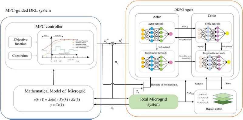
Figure 3 MPC-guided DRL algorithm.

Based on this baseline, the reinforcement learning module adopts the Deep Deterministic Policy Gradient algorithm to interact with the real microgrid environment and generate a compensatory dispatch command, denoted as $u_t^l$. Consequently, the final dispatch command can be expressed as:

$$u_t=u_t^m+u_t^l$$

(17)

This integration combines the global foresight optimization of model predictive control with the real-time decision-making advantages of deep reinforcement learning. Since the baseline command from MPC provides high-quality initial data points for DRL, it effectively narrows DRL’s exploration space and improves sample efficiency. To ensure synchronized collaboration between MPC and DRL, their control periods must be aligned.

3.2 MPC Module

Considering the charging and discharging efficiencies of the battery, the dynamic model of the energy storage charging and discharging process can be expressed as

$$\mathit{SOC}(t)=\{\begin{array}{cc}\mathit{SOC}(t-1)(1-\sigma )+\frac{P_{\mathit{battery}}(t)}{E_b{\eta }_{\mathit{dis}}}\mathrm{\Delta }\tau ,\hfill & P_{\mathit{battery}}(t)>0\hfill \\ \mathit{SOC}(t-1)(1-\sigma )+\frac{{\eta }_{ch}{P}_{\mathit{battery}}(t)}{E_b}\mathrm{\Delta }\tau ,\hfill & P_{\mathit{battery}}(t)\le 0\hfill \end{array}$$

(18)

where $\mathit{SOC}(t)$ and $\mathit{SOC}(t-1)$ represent the state of charge of the battery at time $t$ and time $t-1$, respectively. sigma denotes the self-discharge rate of the battery. $\mathrm{\Delta }\tau$ represents the time interval. $E_b$ denotes the rated capacity of the battery. ${\eta }_{\mathit{ch}}$ and ${\eta }_{\mathit{dis}}$ represent the charging efficiency and discharging efficiency of the battery, respectively. $P_{\mathit{battery}}(t)$ represents the charging or discharging power of the battery at time $t$. In this paper, $P_{\mathit{battery}}(t)<0$ indicates battery discharging, while $P_{\mathit{battery}}(t)>0$ indicates battery charging.

In the MPC model, the battery dynamics are simplified to a linear state update equation by neglecting charging/discharging efficiency, which reduces computational complexity and ensures real-time performance. Although this simplification introduces modeling errors, the subsequent DRL layer compensates for these inaccuracies through online adjustments. By learning from real-time data, the DRL agent corrects deviations caused by the simplified MPC model, ensuring scheduling accuracy without compromising computational efficiency. The simplified equation is as follows:

$$\mathit{SOC}(t)=\mathit{SOC}(t-1)(1-\sigma )+\frac{P_{\mathit{battery}}(t)}{E_b}\mathrm{\Delta }\tau$$

(19)

Selecting the state variable $x={[P_{\mathit{wind}},P_{\mathit{battery}},P_{\mathit{diesel}},\mathit{SOC}]}^T$, the input variable $u={[\mathrm{\Delta }{P}_{\mathit{wind}},\mathrm{\Delta }{P}_{\mathit{battery}},\mathrm{\Delta }{P}_{\mathit{diesel}},P_{\mathit{buy}},P_{\mathit{sell}}]}^T$; and the output variable $y={[P_{\mathit{wind}},P_{\mathit{deisel}},\mathit{SOC}]}^T$, the aforementioned model of the microgrid comprising wind power, photovoltaic power, diesel generator power, an energy storage system, and interaction with the main grid can be expressed in the following state-space form:

$$x(t+1)=Ax(t)+Bu(t)$$
$$y(t)=Cx(t)$$	(20)

where

$$A=\left[\begin{array}{cccc}1& 0& 0& 0\\ 0& 1& 0& 0\\ 0& 0& 1& 0\\ 0& \frac{-\mathrm{△}t}{E_{\mathit{bat}}}& 0& 1-\sigma \end{array}\right],B=\left[\begin{array}{ccccc}1& 0& 0& 0& 0\\ 0& 1& 0& 0& 0\\ 0& 0& 1& 0& 0\\ 0& 0& 0& 0& 0\end{array}\right],$$

$$C=\left[\begin{array}{cccc}1& 0& 0& 0\\ 0& 0& 1& 0\\ 0& 0& 0& 1\end{array}\right].$$

Defining:

$X=\left[\begin{array}{c}x(t+1)\\ \mathrm{⋮}\\ x(t+N)\end{array}\right],U=\left[\begin{array}{c}u(t)\\ \mathrm{⋮}\\ u(t+N-1)\end{array}\right],Y=\left[\begin{array}{c}y(t+1)\\ \mathrm{⋮}\\ y(t+N)\end{array}\right],$

the states within the prediction horizon can be obtained as:

$$X=\overline{A}x(t)+\overline{B}U$$

(21)

where

$\overline{A}=\left[\begin{array}{c}A\\ A^2\\ \mathrm{⋮}\\ A^N\end{array}\right],\overline{B}=\left[\begin{array}{cccc}B& 0& \mathrm{\cdots }& 0\\ \mathit{AB}& B& \mathrm{\cdots }& 0\\ \mathrm{⋮}& \mathrm{⋮}& \mathrm{\ddots }& \mathrm{⋮}\\ A^{N-1}B& \mathrm{\cdots }& \mathit{AB}& B\end{array}\right].$

The corresponding outputs are:

$$Y=\overline{C}x(t)+\mathrm{\Psi }U$$

(22)

where

$$\overline{C}=\left[\begin{array}{c}\mathit{CA}\\ {\mathit{CA}}^2\\ \mathrm{⋮}\\ {\mathit{CA}}^N\end{array}\right],\mathrm{\Psi }=\left[\begin{array}{cccc}\mathit{CB}& 0& \mathrm{\cdots }& 0\\ \mathit{CAB}& \mathit{CB}& \mathrm{\cdots }& 0\\ \mathrm{⋮}& \mathrm{⋮}& \mathrm{\ddots }& \mathrm{⋮}\\ {\mathit{CA}}^{N-1}B& \mathrm{\cdots }& \mathit{CAB}& \mathit{CB}\end{array}\right].$$

Extending the physical constraints of the control variables (3), (6), (10), and (14) over the entire control horizon $N$ yields:

$$A_{u}U\le \overline{U}$$

(23)

where

$$A_u=\left[\begin{array}{c}I\\ -I\end{array}\right],\overline{U}=\left[\begin{array}{c}{U}_{\max }\\ -U_{\min }\end{array}\right],U_{\min }=\left[\begin{array}{c}{u}_{\min }\\ \mathrm{⋮}\\ u_{\min }\end{array}\right],U_{\max }=\left[\begin{array}{c}{u}_{\max }\\ \mathrm{⋮}\\ u_{\max }\end{array}\right].$$

$I$ is the $5N\times 5N$ identity matrix.

Extending the physical constraints of the state variables (2), (5), (9), and (11) over the entire control horizon $N$ yields:

$$A_{x}X\le \overline{X}$$

(24)

where

$$A_x=\left[\begin{array}{c}\hfill M\\ \hfill -M\end{array}\right],A_x=\left[\begin{array}{c}\hfill M\\ \hfill -M\end{array}\right],$$

$$x_{\min }={[P_{\mathit{wind}}^{\min },P_{\mathit{battery}}^{\min },P_{\mathit{diesel}}^{\min },0.05]}^T,$$

$$x_{\max }={[P_{\mathit{wind}\max }^{\mathit{predict}},P_{\mathit{battery}}^{\max },P_{\mathit{diesel}}^{\max },0.95]}^T,$$

$M$ is the $4N\times 4N$ identity matrix.

Substituting Equation (24) into Equation (27) and rearranging gives:

$$\left[\begin{array}{c}\hfill \overline{B}\\ \hfill -\overline{B}\end{array}\right]U\le \left[\begin{array}{c}\hfill X_{\max }-\overline{A}x(t)\\ \hfill -X_{\min }+\overline{A}x(t)\end{array}\right]$$

(25)

The constraints on $X$ and $U$ can described above can be expressed as:

$$\mathit{GU}\le h$$

(26)

where

$$G=\left[\begin{array}{c}I\\ -I\\ \overline{B}\\ -\overline{B}\end{array}\right],h=\left[\begin{array}{c}{U}_{\max }\\ -U_{\min }\\ X_{\max }-\overline{A}x(t)\\ -X_{\min }+\overline{A}x(t)\end{array}\right].$$

The microgrid must satisfy the power balance equation $P_{\mathit{wind}}+P_{\mathit{solar}}^{\mathit{predict}}+P_{\mathit{buy}}-P_{\mathit{sell}}+P_{\mathit{diesel}}+P_{\mathit{battery}}=P_{\mathit{load}}$, Extending this over the prediction horizon gives:

$${\overline{C}}_{\mathit{balance}}X+{\overline{D}}_{\mathit{balance}}U={\overline{d}}_{\mathit{balance}}$$

(27)

where

$${\overline{C}}_{\mathit{balance}}=\mathit{diag}(C_{\mathit{balance}},\mathrm{\dots },C_{\mathit{balance}}),$$

$${\overline{D}}_{\mathit{balance}}=\mathit{diag}(D_{\mathit{balance}},\mathrm{\dots },D_{\mathit{balance}}),$$

$$C_{\mathit{balance}}=[-1,-1,-1,0],$$

$${\overline{D}}_{\mathit{balance}}=diag(D_{\mathit{balance}},\mathrm{\dots },D_{\mathit{balance}}),$$

$$C_{\mathit{balance}}=[-1,-1,-1,0],D_{\mathit{balance}}=[0,0,0,1,-1],$$

$${\overline{d}}_{\mathit{balance}}=\left[\begin{array}{c}{P}_{\mathit{load}}(t+1)-P_{\mathit{solar}}(t+1)\\ \mathrm{⋮}\\ P_{\mathit{load}}(t+N)-P_{\mathit{solar}}(t+N)\end{array}\right].$$

Substituting Equation (25) into Equation (30) yields the equality constraint for $U$:

$$({\overline{C}}_{\mathit{balance}}\overline{B}+{\overline{D}}_{\mathit{balance}})U={\overline{d}}_{\mathit{balance}}-{\overline{C}}_{\mathit{balance}}\overline{A}x(t)$$

(28)

The economic cost $C_1(t)$ defined in Equation (17) can be expanded over the prediction horizon as:

$$\sum _{i=1}^N{C}_1(t+i)=U^T{H}_{C_1}U+f_{C_1}^{T}U$$

(29)

where

$$f_{C_1}=2{\mathrm{\Psi }}^T{Q}_{\mathit{disel}}^T\overline{C}x(t)+{\mathrm{\Psi }}^T{r}_{\mathit{disel}}+{\mathrm{\Psi }}^T{\alpha }_{\mathit{wind}}+f_{\mathit{grid}},$$

$$H_{C_1}={\mathrm{\Psi }}^T{Q}_{\mathit{disel}}\mathrm{\Psi },{\alpha }_{\mathit{wind}}^T=C_{\mathit{inital}}\cdot e^T{S}_{\mathit{wind}},$$

$$Q_{\mathit{disel}}=S_{\mathit{disel}}^{T}a{I}_N{S}_{\mathit{disel}},r_{\mathit{dissel}}^T=b\cdot e^T{S}_{\mathit{disel}},$$

$$f_{\mathit{grid}}={\mathit{price}}_{\mathit{buy}}\cdot S_{\mathit{buy}}^{T}e+{\mathit{price}}_{\mathit{sell}}\cdot S_{\mathit{sell}}^{T}e,$$

$S_{\mathit{wind}}$ is an $N\times 4N$ matrix where each row has a value of 1 at the $4(k-1)+1$ column, $(k=1,\mathrm{\dots },N)$ and zeros elsewhere. Similarly, $S_{\mathit{disel}}$ is an $N\times 4N$ matrix with a value of 1 at the $4(k-1)+3$ column in each row. Furthermore, $S_{\mathit{buy}}$ and $S_{\mathit{sell}}$ are $N\times 5N$ matrices with a value of 1 at the $5(k-1)+4$ and $5(k-1)+5$ column in each row, respectively. The vector $e$ is an N-dimensional column vector.

The safety cost $C_2(t)$ defined in Equation (18), is expanded over the prediction horizon as follows:

$$\sum _{i=1}^N{C}_2(t+i)=U^T{H}_{C_2}U+f_{C_2}^{T}U$$

(30)

where

$$H_{C_2}={\sigma }_1{S}_{\mathrm{\Delta }}^T{S}_{\mathrm{\Delta }}+\kappa S_{\mathit{grid}}^T{D}^{T}D{S}_{\mathit{grid}},$$

$$f_{C_2}=-{\sigma }_2{\mathrm{\Psi }}_{\mathit{SOC}}^{T}e+2\kappa S_{\mathit{grid}}^T{D}^T{d}_0,S_{\mathit{grid}}=S_{\mathit{buy}}-S_{\mathit{sell}},$$

$S_{\mathrm{\Delta }}$ is an $N\times 5N$ matrix with a value of 1 at the $5(k-1)+2$ column in each row.

$$D=\left[\begin{array}{ccccc}1& 0& 0& \mathrm{\cdots }& 0\\ -1& 1& 0& \mathrm{\cdots }& 0\\ 0& -1& 1& \mathrm{\cdots }& 0\\ \mathrm{⋮}& \mathrm{⋮}& \mathrm{\ddots }& \mathrm{\ddots }& \mathrm{⋮}\\ 0& 0& \mathrm{\cdots }& -1& 1\end{array}\right],d_0=\left[\begin{array}{c}-P_{\mathit{grid}}(t-1)\\ 0\\ 0\\ \mathrm{⋮}\\ 0\end{array}\right].$$

$E(t)$ can be expanded over the prediction horizon as:

$$\underset{U}{\min }\sum _{i=1}^{N}E(t+i)=U^T{H}_{E}U+f_E^{T}U$$

(31)

where

$$H_E={\mathrm{\Psi }}^T\mathrm{\Psi },f_E=2{\mathrm{\Psi }}^T(\overline{C}x(t)-Y_{\text{day–ahead}}),$$

$$Y_{\text{day–ahead}}=\left[\begin{array}{c}{y}_{\mathit{day}}(t+1)\\ y_{\mathit{day}}(t+2)\\ \mathrm{⋮}\\ y_{\mathit{day}}(t+N)\end{array}\right],y_{\mathit{day}}(t+k)=\left[\begin{array}{c}{P}_{\mathit{wind}}^{\mathit{day}}(t+k)\\ P_{\mathit{disel}}^{\mathit{day}}(t+k)\\ {\mathit{SOC}}^{\mathit{day}}(t+k)\end{array}\right],$$

$$P_{\mathit{wind}}^{\mathit{day}}(t+k),P_{\mathit{disel}}^{\mathit{day}}(t+k),{\mathit{SOC}}^{\mathit{day}}(t+k)$$

represent the day-ahead dispatch reference power for the diesel generator and the state of charge, respectively, at time step $t+k$.

In summary, the MPC optimization problem can be formulated as the following quadratic programming problem:

$$\underset{U}{\min }\sum _{i=1}^{N}J(t+i)=U^{T}HU+f^{T}U$$
$$s.t.(\text{31}),(\text{34})$$	(32)

where

$$H={\lambda }_1(H_{C_1}+H_{C_2})+{\lambda }_2{H}_E,f={\lambda }_1(f_{C_1}+f_{C_2})+{\lambda }_2{f}_E.$$

The quadratic programming problem described above is solved directly. At each time step, the solver derives the optimal control sequence for the next N steps based on the predictive model and constraints. Using the control variables at the current time step, $u(t)$, defined as $\mathrm{\Delta }{P}_{\mathit{wind}},\mathrm{\Delta }{P}_{\mathit{battery}},\mathrm{\Delta }{P}_{\mathit{diesel}}$, the corresponding predicted values $P_{\mathit{wind}}^m,P_{\mathit{battery}}^m,P_{\mathit{diesel}}^m$ at time $t+1$ can be calculated as follows:

$$P_{\mathit{wind}}^m=P_{\mathit{wind}}(t)+\mathrm{\Delta }{P}_{\mathit{wind}}$$	(33)
$$P_{\mathit{battery}}^m=P_{\mathit{battery}}(t)+\mathrm{\Delta }{P}_{\mathit{battery}}$$	(34)
$$P_{\mathit{diesel}}^m=P_{\mathit{diesel}}(t)+\mathrm{\Delta }{P}_{\mathit{diesel}}$$	(35)

The MPC module then delivers the computed output from the previous step $u_t^m=[P_{\mathit{wind}}^m,P_{\mathit{battery}}^m,P_{\mathit{diesel}}^m]$ to the DRL module. The DRL module receives this input and simultaneously reads real-time measurements from the physical microgrid system, including $P_{\mathit{wind}\max }^{\mathit{real}},\mathit{SOC},P_{\mathit{load}},P_{\mathit{solar}}^{\mathit{real}},t$, these elements form the environment for reinforcement learning. In this way, MPC provides baseline guidance for the agent’s optimization process, which not only narrows the exploration space but also enhances the training efficiency of the reinforcement learning algorithm.

3.3 DRL Module

Since the control variables in microgrid scheduling are all continuous values, the DDPG algorithm suitable for continuous action spaces is adopted. Building upon the baseline scheduling commands provided by MPC module, the DRL module constructs a reinforcement learning environment for the microgrid. Using the Actor-Critic framework for policy training, it ultimately obtains an Actor network capable of outputting real-time compensation values, which then delivers these compensation values online.

3.3.1 Microgrid environment construction

The state of the microgrid at the next time step depends solely on the current state and the decisions made at that time, making its scheduling process a typical Markov Decision Process (MDP). This can be represented by a quintuple $(s,a,P,\gamma ,r)$, where $s$ denotes the environmental state vector, $a$ denotes the action vector, $P$ is the state transition function determined by the environment, $r$ denotes the reward function, and $\gamma$ denotes the discount factor [16–19].

The environment for the DRL module is composed of the $u_t^m$ passed from the MPC module and the actual system information read from the real microgrid environment. It is defined as follows:

$$s_t=(P_{\mathit{wind}}^m,P_{\mathit{battery}}^m,P_{\mathit{diesel}}^m,P_{\mathit{solar}}^{real},\mathit{SOC},P_{\mathit{load}},P_{\mathit{wind}\max }^{\mathit{real}},t)$$

(36)

where $P_{\mathit{wind}\max }^{\mathit{pred}}$ and $P_{\mathit{solar}}^{\mathit{real}}$ represent the actual maximum wind power and photovoltaic power, respectively. Since prediction errors typically follow a zero-mean normal distribution [20, 21], $P_{\mathit{wind}\max }^{\mathit{pred}}$ and $P_{\mathit{solar}}^{\mathit{real}}$ can be expressed as:

$$P_{\mathit{wind}\max }^{\mathit{real}}=\max (0,P_{\mathit{wind}\max }^{\mathit{pred}}[1+{\epsilon }_w])$$	(37)
$$P_{\mathit{solar}}^{\mathit{real}}=\max (0,P_{\mathit{solar}}^{\mathit{pred}}[1+{\epsilon }_s])$$	(38)

where the prediction errors ${\epsilon }_w$ and ${\epsilon }_s$ both follow a normal distribution $N(0,0.1)$.

After reading the environmental information, the agent chooses the appropriate action based on its policy. The action at time step $t$ is defined as:

$$a_t=(P_{\mathit{wind}}^l,P_{\mathit{diesel}}^l,P_{\mathit{battery}}^l)$$

(39)

where $P_{\mathit{wind}}^l,P_{\mathit{diesel}}^l$ and $P_{\mathit{battery}}^l$ are the compensation values for wind turbine power, diesel generator power, and battery power, respectively. The output of the DRL module is the compensation value for microgrid scheduling, i.e.:

$$u_t^l=a_t$$

(40)

According to Formula ((19)), the actual scheduled power of the microgrid is:

$$\{\begin{array}{c}{P}_{\mathit{wind}}=P_{\mathit{wind}}^m+P_{\mathit{wind}}^l\hfill \\ P_{\mathit{diesel}}=P_{\mathit{diesel}}^m+P_{\mathit{disel}}^l\hfill \\ P_{\mathit{battery}}=P_{\mathit{battery}}^m+P_{\mathit{battery}}^l\hfill \\ P_{\mathit{solar}}=P_{\mathit{solar}}^{real}\hfill \\ P_{\mathit{grid}}=P_{\mathit{load}}-P_{\mathit{wind}}-P_{\mathit{desel}}-P_{\mathit{battery}}-P_{\mathit{solar}}\hfill \end{array}$$

(41)

The reward function reflects the objective described by Formula (15) and must also ensure the optimized policy satisfies all operational constraints of the microgrid. The reward is defined as:

$$r_t=-J(t)+H$$	(42)
$$H=\{\begin{array}{cc}500\hfill & g\ge 0\hfill \\ 0\hfill & g<0\hfill \end{array}$$	(45)

Here, $J(t)$ represents the system cost calculated at time $t$ according to Formula (16). $H$ is the reward for actions and states satisfying inequality constraints during operation, where $g\ge 0$ indicates the action and state satisfy the constraints.

3.3.2 Training process

The main DDPG network consists of two deep neural networks, namely the value network (Critic network) $Q(s_t,a_t|{\theta }_Q)$ and the policy network (Actor network) $\mu (s_t|{\theta }_{\mu })$, which are represented by the parameters ${\theta }_Q$ and ${\theta }_{\mu }$ respectively. Aiming to stabilize the training phase, target networks $Q^{\prime }(s_t,a_t|{\theta }_Q^{\prime })$ and ${\mu }^{\prime }(s_t|{\theta }_{\mu }^{\prime })$ are introduced to slowly track the main networks $Q$ and $\mu$.

Critic Network Training: The role of the Critic network is to evaluate the value of taking action $a_t$ in state $s_t$. During training, random noise $\eta$ is added to promote exploration. The action actually executed is:

$$a_t=\mu (s_t|{\theta }_{\mu })+\eta$$

(46)

where $\eta$ employs Gaussian noise and is used only during the training phase.

The Critic network is updated by sampling $N_s$ data tuples $(s_t,a_t,r_t,s_{t+1})$ from the experience replay buffer and minimizing the loss function for parameter updates:

$$L({\theta }_Q)=\frac{1}{N_s}\sum _{t=1}^{N_s}{(y_t-Q(s_t,a_t|{\theta }_Q))}^2$$	(47)
$$L({\theta }_Q)=\frac{1}{N_s}\sum _{t=1}^{N_s}{(y_t-Q(s_t,a_t|{\theta }_Q))}^2$$	(48)

where $y_t=r_t+\gamma Q^{\prime }(s_{t+1},{\mu }^{\prime }(s_{t+1}|{\theta }_{\mu }^{\prime }|{\theta }_Q^{\prime })$ signifies the temporal-difference target, as computed by the target networks. The term $k$ indicates the count of gradient descent iterations, ${\eta }_Q$ denoting the learning rate for the Critic network.

Actor Network Training: The optimal action $a_t$ for a given state $s_t$ is produced by the Actor network. Parameter updates are performed to maximize the anticipated cumulative reward, where the policy gradient is approximated by sampling as:

$${\nabla }_{{\theta }_{\mu }}J({\theta }_{\mu })\approx \frac{1}{N_s}\sum _{t=1}^{N_s}[{\nabla }_{{\theta }_{\mu }}\mu (s_t|{\theta }_{\mu }){\nabla }_{a}Q(s_t,a|{\theta }_Q)]$$

(49)

The update formula for the network parameters is:

$${\theta }_{\mu }^{k+1}={\theta }_{\mu }^k+{\eta }_{\mu }{\nabla }_{{\theta }_{\mu }}J({\theta }_{\mu })$$

(50)

where ${\eta }_{\mu }$ is the learning rate of the Actor network.

Target Network Soft Update: Following the update of the Critic and Actor networks, the parameters of their respective target networks, $Q^{\prime }$ and ${\mu }^{\prime }$ are also softly updated:

$${\theta }_Q^{\prime }\leftarrow \tau {\theta }_Q+(1-\tau ){\theta }_Q^{\prime }$$	(51)
$${\theta }_{\mu }^{\prime }\leftarrow \tau {\theta }_{\mu }+(1-\tau ){\theta }_{\mu }^{\prime }$$	(52)

where $\tau \in [0,1]$ is the soft update coefficient.

3.4 Module Coupling

At time $t-1$, the MPC module calculates $u(k-1)$ based on the current state $x_{t-1}$ to obtain $u_t^m=[P_{\mathit{wind}}^m,P_{\mathit{battery}}^m,P_{\mathit{diesel}}^m]$, which serves as part of the environment input for the DRL module at time $t$. After interacting with the real system, the DRL agent outputs the power compensation amount $u_t^l=[P_{\mathit{wind}}^l,P_{\mathit{diesel}}^l,P_{\mathit{battery}}^l]$. The final execution is $u_t=u_t^m+u_t^l$. The reinforcement learning module then calculates the actual $P_{\mathit{wind}},P_{\mathit{diesel}},P_{\mathit{battery}},\mathit{SOC}$ at time $t$, which is returned to the MPC module as $x_t$ for a new round of optimization. This process can be represented by the following pseudocode.

Algorithm: MPC-guided DRL Strategy

1: Initialization: Initialize system state $x_0$

2: for time step$t=1,2,\mathrm{\dots },Tdo$

3:   The MPC module obtains the reference dispatch command

$u_t^m=[P_{\mathit{wind}}^m,P_{\mathit{battery}}^m,P_{\mathit{diesel}}^m]$ based on the system state at the previous time

step $x_{t-1}$.

4:   The DRL agent interacts with the real system and outputs the power

compensation amount $u_t^l=[P_{\mathit{wind}}^l,P_{\mathit{diesel}}^l,P_{\mathit{battery}}^l]$.

5:   Calculate and execute the final control command : $u_t=u_t^m+u_t^l$.

6:   The DRL module calculates the actual $P_{\mathit{wind}},P_{\mathit{diesel}},P_{\mathit{battery}},\mathit{SOC}$ of the

system at time $t$ and returns them to the MPC module as $x_t$.

7: end for

4 Simulation Results and Discussion

The simulation data is sourced from a 2021 annual operation dataset of an open-access microgrid in Europe. This dataset was acquired using the Supervisory Control and Data Acquisition (SCADA) system and includes electricity prices, meteorological data, load, wind power output, photovoltaic (PV) output, and the power capacity of each microgrid unit. The power capacities and relevant parameters of these units are listed in Table 1.

Table 1 Parameters of each microgrid device

Parameter	Value
$P_{\text{battery–cha}}/P_{\text{battery–discha}}$	120 kW/120 kW
$C_{\mathit{battery}}$	300 kWh
$\mathrm{\Delta }{P}_{\mathit{battery}\max }$	50 kW
$\mathrm{\Delta }{P}_{\mathit{wind}\max }$	50 kW
$P_{\mathit{diesel}}^{\max }$	200 kW
$a/b/c$	0.04/0.94/0.157
$\mathrm{\Delta }{P}_{\mathit{disel}\max }$	40 kW
$P_{\text{grid–sell}}^{\max }/P_{\text{grid–buy}}^{\max }$	200 kW/200 kW
$\beta$	0.6
${\sigma }_1/{\sigma }_2$	0.02/0.6
$\kappa$	0.05
$C_{\mathit{initial}}$	0.05
$P_{\mathit{wind}}^{\max }$	500 kW

In the design of the MPC module, the sampling interval is set to $T_s=15$ min. The prediction horizon is defined as $N=8$ steps, corresponding to a total prediction duration of $T_s\cdot N=2$ hour. This setup ensures that the controller can perform rolling optimization within a reasonable timeframe and output the optimal control command $u_t^m=[P_{\mathit{wind}}^m,P_{\mathit{battery}}^m,P_{\mathit{disel}}^m]$ at each time step, which is then transmitted to the DRL module as environmental information.

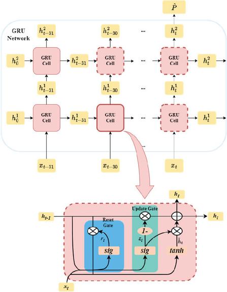
Figure 4 GRU network and cell structure.

Accurate short-term forecasting of renewable generation is essential for microgrid scheduling, as it provides the necessary future information for real-time decision-making. A joint Wind-Solar GRU power prediction model, as illustrated in Figure 4, is constructed to simultaneously predict short-term wind and PV power [22, 23]. To maintain consistency with the MPC optimization requirements, the joint prediction model outputs a combined wind-solar power sequence for the next 2 hours. Historical power data from the previous 8 hours is selected as the model input, corresponding to 32 time steps.

At time $t$, the input sequence for the GRU network consists of 32 time steps, where the input vector for each time step is defined as:

$$x_{t-k}=[P_{\mathit{wind}}(t-k),P_{\mathit{soalr}}(t-k)],k=0,1,\mathrm{\dots },31$$

(53)

The full input sequence for the GRU network is:

$$X_t=[x_{t-31},x_{t-30},\mathrm{\dots },x_t]$$

(54)

The GRU network outputs the predicted wind-solar joint power sequence for the following 8 time steps through a non-linear mapping function $f(\cdot )$:

$$\widehat{P}=[\widehat{P}(t+1),\widehat{P}(t+2),\mathrm{\dots },\widehat{P}(t+8)]$$

(55)

where $\widehat{P}(t+i)=[{\widehat{P}}_{\mathit{wind}}(t+i),{\widehat{P}}_{\mathit{solar}}(t+i)],i=1,2,\mathrm{\dots }8$.

The output sequence of the GRU network is temporally aligned with the MPC controller and serves as a known input within the MPC prediction horizon. As illustrated, the network architecture comprises two hidden layers, with the first and second layers consisting of 128 and 256 neurons, respectively. To mitigate overfitting, a dropout mechanism is implemented after each hidden layer, with dropout rates configured at 0.3 and 0.4. The training batch size for the model is set to 64.

4.1 DRL Training

The Actor-Critic networks within the DRL module both utilize a Multi-Layer Perceptron (MLP) structure with three hidden layers. Specifically, these three hidden layers contain 225, 180, and 160 neurons, respectively. The Rectified Linear Unit (ReLU) is adopted to activate the hidden layers, with the Softmax function being applied to the policy network’s output layer. The specific hyperparameter configurations are detailed in Table 2.

Table 2 Hyperparameters of deep reinforcement learning

Hyperparameter	Value
Experience replay buffer	${10}^5$
Mini-batch size $N_s$	64
Discount factor $\gamma$	0.99
Critic network learning rate ${\theta }_Q$	0.001
Actor network learning rate ${\theta }_{\mu }$	0.0001
Soft update coefficient $\tau$	0.001
Training episodes	1500

To validate the superiority of the proposed algorithm, a standalone MPC controller and a DRL controller were designed to perform intraday scheduling optimization on the same microgrid system. The parameter settings for the standalone MPC are identical to those of the MPC module in the MPC-guided DRL controller. The standalone DRL module interacts directly with the microgrid system to output the final execution power. The state of the environment is defined as: $s_t=(P_{\mathit{load}},\mathit{SOC},P_{\mathit{wind}\max }^{\mathit{pred}},P_{\mathit{solar}}^{\mathit{pred}},t)$, The action is defined as: $a_t=(P_{\mathit{wind}},P_{\mathit{disel}},P_{\mathit{battery}})$. To ensure a fair comparison, the Actor-Critic network structure is identical to that in Equation (42).

The simulation code is implemented in a Python 3.10 environment based on the PyTorch framework. All simulation tests were conducted on a Windows system with a 2.5 GHz Intel Core-i5 processor and 16 GB of RAM.

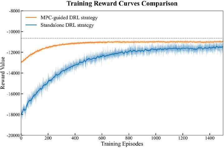
Figure 5 Training reward.

Using 297 days of microgrid operational data from January 1 to October 24, the Actor–Critic network was trained, and the reward trajectories of the standalone DRL strategy and the proposed MPC-guided DRL strategy are presented in Figure 5. As shown in the figure, the MPC-guided DRL strategy achieves higher rewards than the standalone DRL strategy at the very beginning of the training process. With the increase in training episodes, the reward of the MPC–guided DRL strategy rises rapidly and stabilizes at approximately 200 episodes, exhibiting only minor fluctuations thereafter. In contrast, the standalone DRL strategy demonstrates a slower reward improvement and undergoes pronounced oscillations over a considerably longer training period. This behavior is attributed to the fact that, within the MPC-guided DRL framework, the MPC module provides reliable baseline references for the power outputs of the wind turbine, diesel generator, and battery energy storage system. The DRL agent therefore only needs to perform compensatory adjustments on top of this baseline, which significantly narrows the exploration space. Such guidance effectively reduces the stochasticity of policy updates and mitigates ineffective exploration and policy instability.

In the later stages of training, although both methods eventually converge, it is evident that the MPC-guided DRL strategy attains a higher steady-state reward. This is because the MPC module enables the DRL agent to explore efficiently around a high-quality initial policy, thereby facilitating further performance improvement. Conversely, the standalone DRL strategy lacks such prior knowledge and relies predominantly on random trial-and-error exploration, making it more susceptible to convergence to suboptimal local minima and resulting in a lower final reward.

After completing the training of the Actor network, it is deployed in the practical microgrid scheduling system to evaluate its operational performance under real-world conditions.

4.2 Real-time Scheduling Results

The intraday scheduling is performed based on the microgrid data from October 25, utilizing the joint prediction results of wind and solar power from the aforementioned GRU network, as shown in Figure 6. These results serve as known information input for the MPC module to construct the optimization problem within the prediction horizon. To maintain consistency with the control period of the MPC, the day-ahead scheduling results, as illustrated in Figure 7, are expanded in the time dimension to function as reference tracking targets for the intraday scheduling.

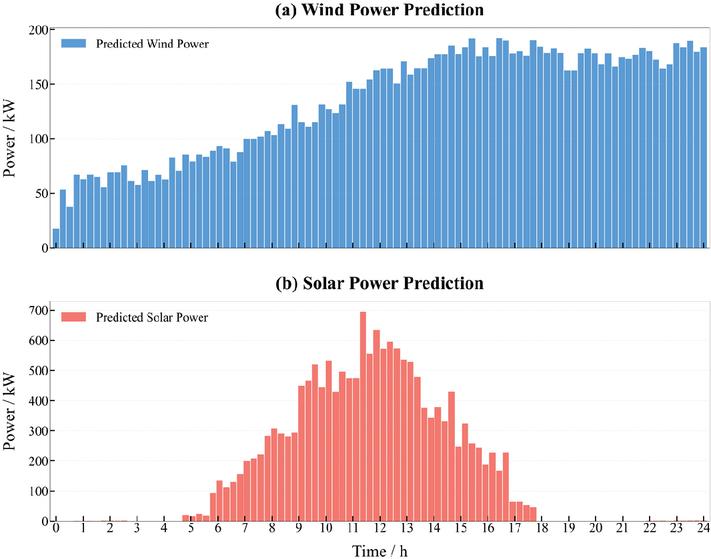
Figure 6 Joint prediction results of wind and solar power.

The intraday scheduling results of the MPC strategy, the DRL strategy, and the MPC-guided DRL strategy are shown in Figures 7, 8, and 9, respectively.

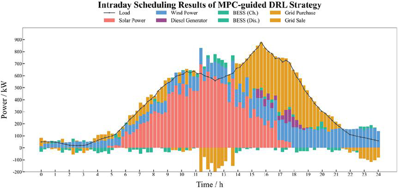
Figure 7 Intraday scheduling results of the MPC strategy.

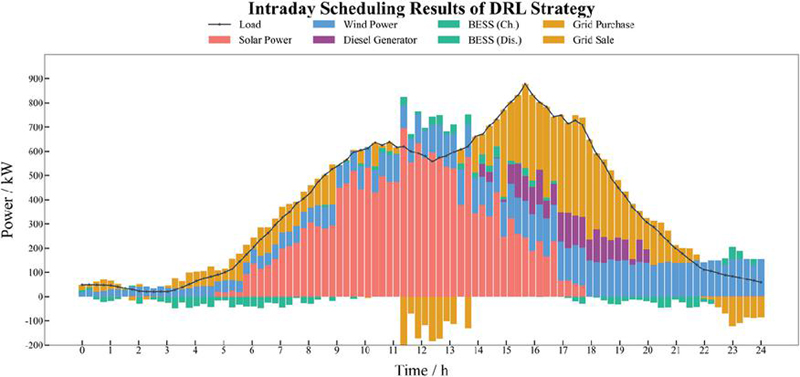
Figure 8 Intraday scheduling results of the standalone DRL strategy.

Figure 9 Intraday scheduling results of the MPC guided DRL strategy.

Figures 7–9 indicate that all three strategies achieve reasonable scheduling performance. When the load demand exceeds the microgrid’s supply capability, the microgrid purchases electricity. While renewable energy generation significantly surpasses the load demand and the electricity price is high (08:00–13:00), the battery charges to increase renewable energy utilization, and the surplus power is sold to the main grid. As wind and photovoltaic generation decline at 14:00, the battery switches to discharge mode to compensate for the supply deficit. During the peak price period (15:00–20:00), the diesel generator increases its output to reduce grid-purchasing costs.

Compared with the standalone MPC strategy, the MPC-guided DRL method shows more flexible adjustment of battery charging and discharging, leading to improved utilization of renewable energy. In contrast, the standalone DRL strategy tends to dispatch the diesel generator and battery more frequently, resulting in relatively larger power fluctuations. By integrating the stability of MPC with the adaptive capability of DRL, the MPC-guided DRL strategy achieves a more balanced power allocation among renewable generation, storage, and conventional generation. To comprehensively evaluate the performance of different optimization strategies, Table 3 lists the key metrics under the MPC, DRL, and MPC-guided DRL methods. This table includes wind power utilization, average diesel generation, average battery charging/discharging power, and total cost.

Table 3 Comparison of key metrics

Metric	MPC	MPC $+$ DRL	DRL
Wind Power Utilization (%)	76.31	86.92	78.0
Avg. Diesel Power (kW)	10.34	8.61	22.13
Avg. Battery Power (kW)	20.94	10.71	22.40
Total Cost	12450	11209	11505

As shown in Table 3, the MPC-guided DRL method achieves the best performance across all evaluation metrics. Compared with the standalone MPC strategy, this method increases wind power utilization by 10.61% and reduces the total operating cost by 11.42%. In addition, the average battery power is maintained at a moderate level, indicating that the proposed strategy can effectively coordinate the charging and discharging behavior of the battery while avoiding excessive cycling. Although the standalone MPC strategy can theoretically obtain an optimal solution based on the system model, it relies on a simplified linear model during practical implementation, and forecasting errors in wind and solar generation are unavoidable. Consequently, its scheduling results often deviate from the true optimal solution in real operating conditions, leading to insufficient utilization of renewable energy. In contrast, within the MPC-guided DRL framework, the DRL agent serves as a compensation module that performs online corrections to the MPC outputs. By continuously interacting with the real environment, the DRL agent mitigates the limited adaptability of standalone MPC, thereby significantly improving the utilization of renewable resources and overall economic performance.

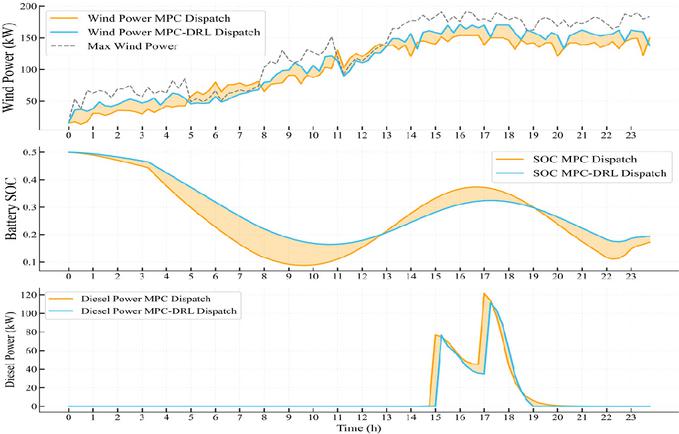
Figure 10 Comparison between MPC strategy and MPC-guided DRL strategy.

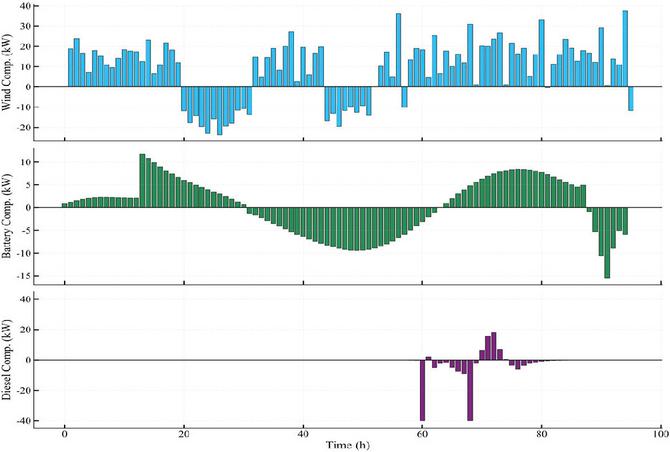
Figure 11 Compensation amount of DRL module.

Compared with the standalone DRL strategy, the MPC-guided DRL method also demonstrates clear advantages, with wind power utilization increased by 8.92% and total operating cost reduced by 4.14%. This improvement can be attributed to the limited policy quality of standalone DRL when no high-quality initialization is provided by MPC. As illustrated in Figure 5, the cumulative reward obtained by standalone DRL is significantly lower than that of the MPC-guided DRL strategy. In practical scheduling, due to the lack of effective guidance from MPC, standalone DRL struggles to achieve an optimal trade-off under complex operational constraints. As a result, it tends to perform more frequent control actions, including excessive dispatch of the diesel generator and battery storage system. This not only increases operating costs but also introduces additional risks to system safety and stability.

Figure 10 presents the wind power generation, battery state of charge, and diesel generation power under the MPC policy and the MPC-guided DRL policy. Figure 11 illustrates the compensation power provided by the DRL module at each time step.

Figure 10 demonstrates that, compared to the MPC method which relies solely on predictive models, the MPC-guided DRL strategy effectively mitigates the impact of deviations between actual wind power output and predicted values on scheduling performance. This leads to a more comprehensive and rational utilization of wind power resources.

Between 14:00 and 23:00, when actual wind power exceeds the MPC predicted levels, the DRL module further increases wind power output based on the MPC baseline schedule, bringing it closer to the maximum available level and improving the wind power curtailment rate. Conversely, when actual wind power is lower than the MPC predictions, the DRL module reduces the wind power output accordingly, restricting it within a feasible range to avoid scheduling infeasibility or system operational risks caused by strictly tracking inaccurate predictions.

Furthermore, by incorporating a penalty term for battery power fluctuations in the DRL reward function, the agent effectively suppresses frequent charging and discharging of the energy storage system while optimizing wind power utilization. This results in a smoother change in the battery’s State of Charge. Overall, the MPC-guided DRL strategy enhances renewable energy integration while reducing the frequency of energy storage cycles, thereby achieving more stable and economical operation.

5 Conclusion

This paper proposes an MPC-guided DRL scheduling strategy for microgrids, which integrates the predictive capability of model predictive control with the adaptability of deep reinforcement learning to address the uncertainty associated with wind and solar power in energy management. A microgrid model composed of wind power, photovoltaic generation, energy storage, a diesel generator, and the main grid is established, and three strategies – MPC-guided DRL, standalone MPC, and standalone DRL – are employed for day-ahead scheduling simulations. The experimental results demonstrate that the proposed MPC-guided DRL strategy effectively reduces operating costs, mitigates fluctuations in the battery state of charge, and enhances the utilization of renewable energy. In addition, the strategy is evaluated under various environmental conditions, showing good robustness and environmental adaptability. Therefore, the proposed algorithm provides a highly promising intelligent optimization approach for microgrids.

References

1. T. Appenzeller, 2025 Breakthrough of the Year, J. Science, 2025.

2. Li, G., Ji, S., Wang, M., et al. Research on Optimization and Scheduling Control Strategy of Renewable Energy Grid-Connection Based on Intelligent Control. J. Distributed Generation & Alternative Energy Journal, 41(01) 83–100.

3. Zhang Z, Guo L, Wu J, et al. Optimization of microgrid dispatching by integrating photovoltaic power generation forecast. J. Sustainability, 2025, 17(2) 648.

4. Xu, H. B., Yue B., and Zhang F. 2026. Optimal configuration of hybrid energy storage capacity for wind power fluctuation smoothing based on GSWOA-VMD. J. Distributed Generation and Alternative Energy. 41(01) 167–192..

5. Kumar K, Kwon S, Bae S. Deep reinforcement learning-based control strategy for integration of a hybrid energy storage system in microgrids. J. Journal of Energy Storage, 2025, 108: 114936

6. Shu, Y. K., W. Z. Bi, W. Dong, et al. Dueling Double Q-learning based Real-time Energy Dispatch in Grid-connected Microgrids. C. 2020 19th International Symposium on Distributed Computing and Applications for Business Engineering and Science (DCABES). IEEE, 2020.

7. Kuang, Y. J., D. H. Zhou, Z. W. Shen, et al. Proximal Policy Optimization-Based Reinforcement Learning Control of Single-Stage Multiport Inverter in Islanded Microgrids. J. IEEE Transactions on Industrial Electronics, 2026, 73(4) 5663–5674

8. Liu, Y. L., T. H. Qie, Y. Yu, et al. A Novel Integral Reinforcement Learning-Based Control Method Assisted by Twin Delayed Deep Deterministic Policy Gradient for Solid Oxide Fuel Cell in DC Microgrid. J. IEEE Transactions on Sustainable Energy, 2023, 14(1) 688–703.

9. Li Y, He S, Li Y, et al. Federated multiagent deep reinforcement learning approach via physics-informed reward for multi-microgrid energy management. J. IEEE Transactions on Neural Networks and Learning Systems, 2024, 35(5) 5902–5914.

10. Mo, S. Y., W. H. Chen, W. X. Zheng, et al. Distributed Hybrid Control for Heterogeneous Multiagent Systems With Variable Communication Delays and Its Application to DC Microgrids. J. IEEE Transactions on Systems, Man, and Cybernetics: Systems, 2023, 53(12) 7501–7512.

11. X. Kong, X. Liu, L. Ma, and K. Y. Lee, Hierarchical distributed model predictive control of standalone wind/solar/battery power system. J. IEEE Trans. Syst. Man Cybern. Syst., vol. 49, no. 8: 1570–1581, Aug. 2019.

12. Z. Zhao, J. Xu, Y. Lei, C. Liu, et al. Robust dynamic dispatch strategy for multi-uncertainties integrated energy microgrids based on enhanced hierarchical model predictive control. J. Applied Energy, 2025, 381: 125141.

13. Wu L, Yin X, Pan L, Liu J. Economic model predictive control of integrated energy systems: A multi-time-scale framework. J. Applied Energy, 2022, 328: 120187

14. Zhu Z, Dong G, Lou Y, et al. MPC-guided deep reinforcement learning for optimal charging of lithium-ion battery with uncertainty. J. IEEE Transactions on Transportation Electrification, 2025.

15. Sun D, Jamshidnejad A, De Schutter B. A novel framework combining MPC and deep reinforcement learning with application to freeway traffic control. J. IEEE Transactions on Intelligent Transportation Systems, 2024, 25(7) 6756–6769.

16. E.H. Sumiea, S.J. Abdulkadir, H.S. Alhussian, S.M. Al-Selwi, A. Alqushaibi, M.G. Ragab, S.M. Fati, Deep deterministic policy gradient algorithm: A systematic review, J. HELIYON, 10 (2024): 30697.

17. Ko, M. S., H. Zhu, and K. Hur. Deterministic and Probabilistic Forecasting of Wind Power Generation and Ramp Rate With Expectation-Implemented Deep Learning. J. IEEE Transactions on Sustainable Energy, 2026, 17(1) 338–350.

18. Lee S, Seon J, Sun Y G, et al. Novel architecture of energy management systems based on deep reinforcement learning in microgrid. J. IEEE Transactions on Smart Grid, 2024, 15(2) 1646–1658.

19. Wu J, Wei Z, Li W, et al. Battery thermal-and health-constrained energy management for hybrid electric bus based on soft actor-critic DRL Algorithm. J. IEEE Transactions on Industrial Informatics, 2021, 17(6) 3751–3761.

20. Zhang, Z. S., Y. Z. Sun, D. W. Gao, et al. A Versatile Probability Distribution Model for Wind Power Forecast Errors and Its Application in Economic Dispatch. J. IEEE Transactions on Power Systems, 2013, 28(3) 3114–3125.

21. Meijie Liu, Peng Qiu, Kai Wei. Research on Wind Speed Prediction of Wind Power System Based on GRU Deep Learning. Preprints of the 3rd IEEE Conference on Energy Internet and Energy System Integration. C. Changsha, China: IEEE, 2019.

22. Lu, C. Q., J. Li, G. D. Zhang, et al. A GRU-based short-term multi-energy loads forecast approach for integrated energy system. Proceedings of the 4th Asia Energy and Electrical Engineering Symposium. C. Chengdu, China, 2022.

23. Yidi, W., Xiaotian, M., Mengyu, L., et al. A New Representative Power Station Selection Method in Distributed Photovoltaic Cluster Power Forecasting. J. Distributed Generation & Alternative Energy Journal, 40(05-06): 1183–1208.

Biographies

Yilu Zhang, female, born in May 2000. She pursued her Bachelor’s degree in Automation at North China Electric Power University from 2019 to 2023 and has been studying for a Master’s degree at the same university since 2023. During her master’s studies, she primarily participated as a researcher in the China-Egypt government joint research project on power grid frequency regulation and in an industry-collaborative project on model predictive control for wind turbines. Her main research focus is on deep learning-based microgrid energy management.

Xiaobing Kong, female, was born in February 1987. She received her bachelor’s, master’s, and doctoral degrees from North China Electric Power University in 2008, 2011, and 2014, respectively, and served as a visiting scholar at Baylor University from 2013 to 2014. She was appointed as a lecturer in 2014, promoted to associate professor in 2020, and has been a master’s supervisor since 2017. She is a member of the IEEE Power & Energy Society and a committee member of the Chinese Association of Automation Youth Committee.

Distributed Generation & Alternative Energy Journal, Vol. 41_3, 655–686
doi: 10.13052/dgaej2156-3306.4136
© 2026 River Publishers