Harmonic Disturbance Identification and Suppression Method Under Compound Power Quality Disturbance
Zhiquan Liu1, Jun Su1, 2,*, Chaolong Tang1 and Yaoyi Wu1
1School of Electrical Engineering and Automation, Xiamen University of Technology, Xiamen, Fujian Province, China, 361012
2Xiamen Key Laboratory of Frontier Electric Power Equipment and Intelligent Control, Xiamen, Fujian Province, China, 361012
E-mail: junsu1989@163.com
*Corresponding Author
Received 07 March 2026; Accepted 17 July 2026
Abstract
High photovoltaic penetration introduces coupled power-quality disturbances whose overlapping RMS, harmonic, and transient signatures are difficult to distinguish under noise. This study develops a field-calibrated diagnosis-and-mitigation workflow for distributed photovoltaic systems. A balanced 17-class dataset is synthesized within IEEE Std 1159-2019 phenomenon ranges. The 50 Hz signals are sampled at 2 kHz for 0.2 s, and additive white Gaussian noise is applied. Magnitude and signed S-transform maps form complementary inputs to a two-channel convolutional neural network. Its learned representation and posterior vector are fused with physically interpretable time, frequency, and time-frequency descriptors. A Logistic-map chaos search then tunes a decision-tree ensemble and probability-fusion weights. Under the unified main condition of 20 dB SNR, 200 samples per class, and stratified source-isolated five-fold cross-validation, the method achieves 97.59% 0.38% accuracy. Ablation and benchmark tests distinguish the contributions of CNN feature learning, conventional ensemble classification, and chaos-optimized fusion. The diagnostic output is mapped to a harmonic-bearing decision and an order-resolved spectrum descriptor, which guide passive target orders and active-current sharing in an equivalent hybrid active power filter (HAPF) model. Using the same field-calibrated PCC waveform, the HAPF reduces current THD from 6.550% to 0.973% and lowers active-converter RMS current from 60.18 A for APF-only operation to 26.40 A, a 56.1% reduction. The source-isolation rule also prevents leakage between training and testing operating conditions. The workflow therefore links reproducible compound-disturbance diagnosis with lower-capacity harmonic mitigation and is directly relevant to power-quality management in distributed photovoltaic generation.
Keywords: Power quality disturbance, harmonic identification, S-transform, convolutional neural network, chaos-optimized ensemble decision tree, hybrid active power filter.
1 Introduction
With the widespread integration of nonlinear loads and distributed energy resources into modern power systems, power quality (PQ) issues in distribution networks have become increasingly complex [1], presenting unprecedented challenges for traditional grids. Distributed generation technologies – primarily based on solar and wind energy – exhibit stochastic fluctuations and nonlinear output characteristics, which have a growing impact on power quality. These impacts manifest in the persistent deterioration of voltage transients, frequency deviations, and harmonic interference [2]. Such PQ disturbances not only compromise the safety and reliability of electrical equipment but also threaten the stable operation of power systems [3].
As modern power network topologies grow more intricate, a disturbance occurring at any location can propagate and couple through the grid, potentially affecting other areas and giving rise to novel disturbance forms [4]. PQ disturbances within the system increasingly manifest not as isolated events but as composite disturbances – simultaneous superpositions of different types of singular events – thus significantly escalating the difficulty of detection and classification [5, 6]. Therefore, it is essential to upgrade traditional PQ disturbance recognition methods to enable accurate and efficient identification, thereby enhancing the power grid’s resilience against disturbances, ensuring the safe and stable operation of electrical equipment, and reducing economic losses caused by power quality issues [7].
The identification of PQ disturbances typically involves two critical steps: feature extraction and signal classification [8].
In feature extraction: Accurate extraction of signal features forms the foundation for effective PQD recognition and classification. Meanwhile, recent studies have shown that a key evolution in feature extraction is the movement from deterministic, hand-crafted metrics to adaptive representations that are learned or optimized from data itself. Ren and Ye [9] proposed a classification framework based on multi-domain parallel feature extraction combined with an optimization strategy. By fusing diverse features and selecting an optimal subset using mutual information and Fisher score, the method enhances representation completeness while mitigating feature redundancy. He et al. [10] developed a PQD feature extraction method based on variational mode decomposition (VMD) optimized through particle swarm optimization (PSO), with improvements including mirror extension to reduce endpoint effects and feature construction via peak value and power spectrum entropy of intrinsic mode functions. Shao et al. [11] introduced a data-driven approach for automatic PQD feature extraction using fast iterative filtering (FIF), which decomposes non-stationary signals without prior knowledge. By incorporating fast Fourier transform (FFT) for efficiency, the method enables real-time PQD recognition and provides interpretable latent representations, demonstrating strong performance across synthetic signals compliant with IEEE 1159-2019. Zhang et al. [12] proposed a power quality disturbance identification method combining the Markov Transition Field (MTF) and deep residual network (ResNet), where the MTF encodes one-dimensional time series into two-dimensional visual representations, and ResNet performs feature extraction and classification. Sampurna et al. [13] conducted a comparative analysis of feature extraction methods for power quality classification using a MATLAB-generated dataset with added noise. Both Stockwell Transform and FFT were evaluated in combination with machine learning classifiers such as k-Nearest Neighbors, Decision Trees, and Bagged Trees. The study offers detailed insights into the performance differences of these techniques in noisy environments, highlighting their applicability to practical PQ disturbance classification. Wang et al. [14] proposed an enhanced feature extraction algorithm for substation equipment image alignment by optimizing the Super Point framework. The method incorporates edge feature fusion via the Canny operator and employs K-means segmentation to guide extraction toward salient target regions, reducing background interference. Experimental results on the CAO-C2F dataset demonstrated a 12.04% improvement in alignment accuracy and reduced processing time, confirming the method’s robustness and efficiency in complex substation scenarios. Meena et al. [15] presented a PQD classification method that employs discrete wavelet transform (DWT) for extracting features from both simple and compound disturbances. Support Vector Machines (SVM) were used for classification, and various feature vector configurations were tested to improve accuracy. The results demonstrated high precision in detection and classification, validating the effectiveness of the DWT-SVM combination for PQ analysis.
In signal classification: Traditional classification approaches typically involve feature extraction via signal processing techniques followed by classification using machine learning models. However, these methods often exhibit limited accuracy when dealing with complex or mixed-type disturbances [16]. In recent years, deep learning methods have attracted significant attention due to their superior ability to automatically extract relevant features. Yong et al. [17] developed a power quality disturbance identification approach combining wavelet transform (WT) and multi-level local density clustering (LDC). The method extracts wavelet energy-based features and utilizes LDC to construct a classification model capable of identifying both single and composite disturbances. Experimental validation demonstrated that the proposed method offers high recognition accuracy with low computational complexity and time consumption. Liao and Liu [18] proposed a disturbance identification method that integrates an optimized VMD with a CNN-BiGRU architecture enhanced by a multi-head attention mechanism. The chaotic Crayfish Optimization Algorithm (COA) was employed to fine-tune VMD parameters, enabling effective extraction of time-domain features from intrinsic mode functions. Kumar et al. [19] addressed the detection of multiple and multistage power quality disturbances by employing a standard S-Transform technique with optimally tuned Gaussian window parameters. By generating synthetic signals based on IEEE-1159 standards, the method effectively distinguishes between complex disturbance types, demonstrating strong performance in the identification of overlapping and sequential PQ events. Guo et al. [20] introduced a transient power quality disturbance classification method based on digital image processing techniques, including gamma correction, edge detection, and local extremum analysis. By converting disturbance signals into grayscale images through normalization and extracting their morphological features, the method enables accurate and efficient classification of transient events, showing improved accuracy over traditional approaches.
Above studies reveal a tension between representation capacity and interpretability: while deep neural networks offer superior performance in feature learning, their outputs are often opaque; conversely, classical classifiers like decision trees are more interpretable but limited in adaptability. At the same time, effective model optimization under nonconvex, noisy, and multidimensional conditions remains an open challenge. Therefore, this paper proposes to combine the feature learning ability of deep learning with the ability of ensemble learning to enhance the adaptability of models to nonlinear disturbances. The key contributions of this paper are outlined below:
• A two-channel CNN is used to learn complementary magnitude and signed S-transform representations. Its 128-dimensional deep representation and 17-dimensional posterior vector are fused with 97 physically interpretable features, after which a Logistic-map chaos search optimizes the decision-tree ensemble and probability-fusion parameters.
• The recognition output is organized into a harmonic-bearing decision and an order-resolved spectrum descriptor. These outputs guide the selection of passive target orders and the rating of the active compensation branch, thereby connecting compound-disturbance diagnosis with a field-calibrated HAPF mitigation study.
2 Harmonic and Disturbance Model Generation
2.1 Field-Measured Harmonic Characteristics
Photovoltaic (PV) grid-connected inverters, functioning as essential power electronic interfaces, inevitably induce voltage fluctuations and harmonic distortions at the point of common coupling (PCC) due to impedance interactions with the power grid. This study investigates an industrial rooftop distributed PV generation system comprising 1,120 optimally configured 660 Wp PV modules. The architecture adopts a modular string design, integrating multiple strings into eight identical 100 kW grid-connected inverter units. The aggregated AC output is centralized and subsequently elevated from 0.4 kV to 10 kV via existing step-up transformers for integration into the distribution network. The corresponding ETAP simulation model is illustrated in Figure 1.
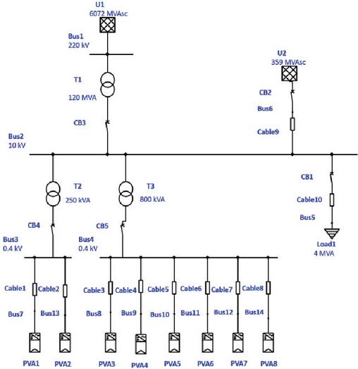
Figure 1 ETAP model of the field-measured grid-connected PV system.
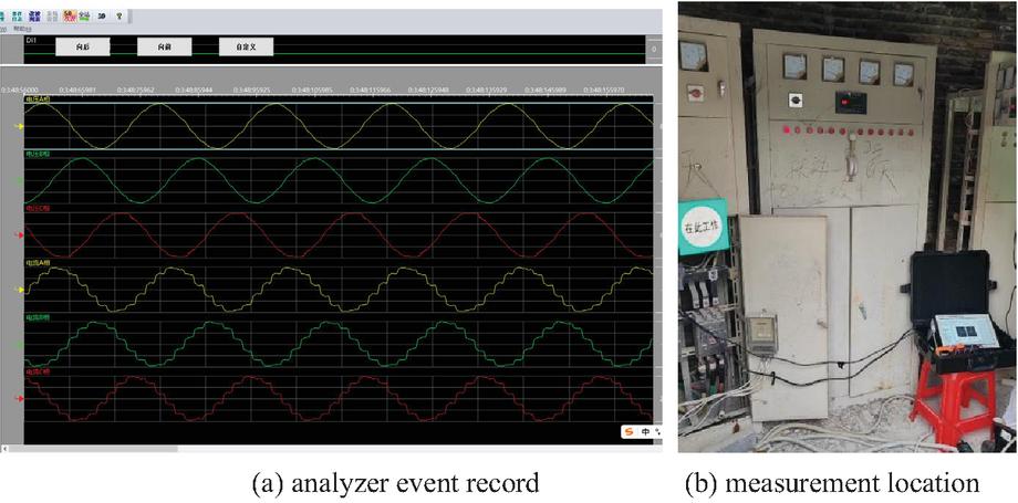
Figure 2 Field measurement at the Cable9 PCC.
Field measurements were acquired at Cable9, the 10 kV incoming feeder at the point of common coupling (PCC). The power-quality analyzer reports a current THD of 6.59%, with 5th, 7th, 11th, and 13th harmonic ratios of 2.0249%, 2.0615%, 4.8523%, and 3.0745%, respectively. The total harmonic distortion rate of the current at the 10kV public connection point is limited to 5%, which has exceeded the standard allowable range. Figure 2 documents the on-site analyzer record and measurement location. The Cable9 current waveform exported by the analyzer was then imported into MATLAB for a 50 Hz-window FFT analysis; the resulting field-data post-processing is presented in Figure 3 and is distinct from the ETAP network model shown in Figure 1. Resampling the exported waveform and applying the common 2nd-25th-order estimator gives a reproducible THD of 6.550%, which is used as the initial condition for all mitigation comparisons in Section 4.2.
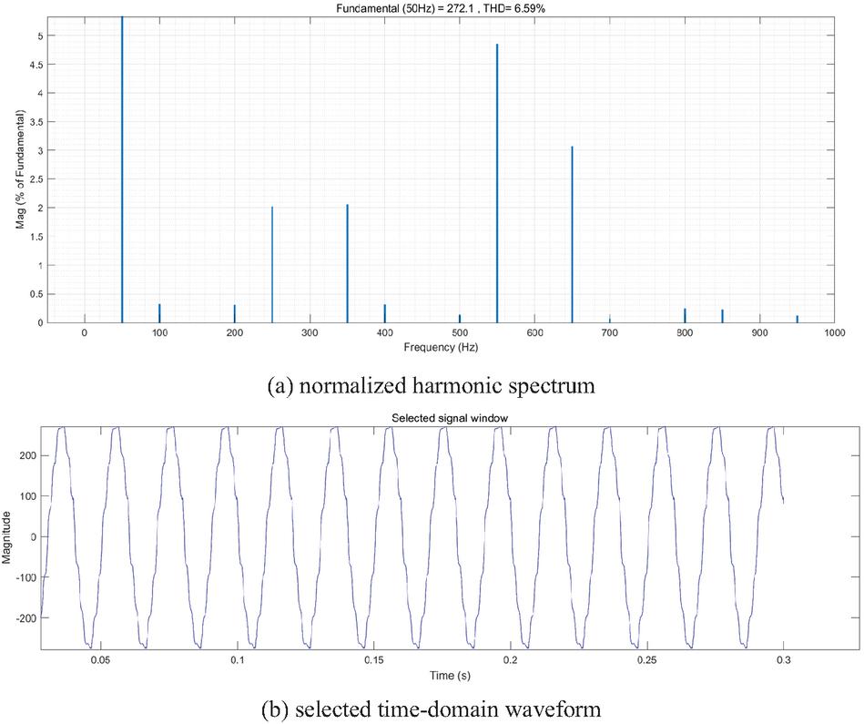
Figure 3 MATLAB post-processing of the field-recorded Cable9 current.
2.2 Single-Disturbance Models
Because a limited field record cannot cover the operating variability required for supervised learning, the formal main dataset was generated in MATLAB using field-calibrated harmonic ratios and IEEE-constrained disturbance parameters. It contains 17 balanced classes and 200 samples per class, giving 3,400 samples in total. For the sample-size sensitivity study, nested class-wise subsets of 100,200, and 300 samples were taken from the same mother source pool, so that changes in sample quantity were not confounded with newly randomized operating conditions. Additive white Gaussian noise was scaled from the variance of each clean waveform; 20 dB was used for the main experiment. Every source case was assigned a persistent SourceID, and samples derived from the same source condition were kept in the same outer fold.
The transformation of periodic electrical parameters into harmonic components is achieved through discrete Fourier transform (DFT) implementation. Periodic electrical quantities with harmonic characteristics can be mathematically represented through Fourier series expansion, decomposing complex waveforms into constituent sinusoidal and cosinusoidal components. The generalized Fourier series expansion formula is expressed as:
| (1) |
To preserve the measured harmonic signature while introducing realistic operating variation, the 5th, 7th, 11th, and 13th harmonic ratios are sampled from truncated normal distributions centered at 2.0249%, 2.0615%, 4.8523%, and 3.0745%, respectively, with each ratio bounded within 25% of its measured center. Independent random phase angles are assigned to the four harmonics. The resulting harmonic class is denoted C1.
| (2) |
Where , and represent the amplitudes of the 5th, 7th, 11th, and 13th harmonics, respectively, while , and denote the corresponding phase angles.
In order to be able to identify normal waveforms and harmonics, a conventional sine wave is introduced. Its signal model is , and the identification number is C0.
The remaining six single-disturbance phenomena are defined using constrained subsets of the categories and terminology in IEEE Std 1159-2019 [21], which provides consistent descriptions of conducted electromagnetic phenomena and deviations from nominal power-system conditions. Each disturbance is assigned a unique identifier from C2 to C7.
Table 1 Single-disturbance types and identifiers
| Identifier | Disturbing Type | Signal model |
| C2 | Voltage Sag | |
| C3 | Voltage Swell | |
| C4 | Voltage Interruption | |
| C5 | Voltage Flicker | |
| C6 | Oscillatory Transient | |
| C7 | Impulsive Transient |
2.3 Compound-Disturbance Models
In addition to the seven single power quality disturbances mentioned above, this paper also includes six double disturbances and three triple disturbances that incorporate harmonics. The corresponding mathematical models and parameter descriptions are shown in Table 2.
Table 2 Compound-disturbance types and identifiers
| Identifier | Disturbing Type |
| C8 | Voltage Sag + Harmonics |
| C9 | Voltage Swell + Harmonics |
| C10 | Voltage Interruption + Harmonics |
| C11 | Voltage Flicker + Harmonics |
| C12 | Oscillatory Transient + Harmonics |
| C13 | Impulsive Transient + Harmonics |
| C14 | Voltage Sag + Harmonics + Oscillatory Transient |
| C15 | Voltage Swell + Harmonics + Oscillatory Transient |
| C16 | Voltage Flicker + Harmonics + Impulsive Transient |
All waveforms have a 50 Hz fundamental frequency and are sampled at 2 kHz for 0.2 s (10 fundamental cycles and 401 points including both endpoints). RMS-event duration is 0.02–0.16 s; sag residual voltage is 0.15–0.85 p.u.; swell magnitude is 1.15–1.75 p.u.; and interruption residual voltage is 0.01–0.08 p.u. Flicker depth and frequency are 0.04–0.07 p.u. and 5–15 Hz. Oscillatory transients use amplitudes of 0.20–0.50 p.u., frequencies of 300–900 Hz, durations of 8–50 ms, and decay constants of 8-20 ms. Impulsive transients use absolute amplitudes of 0.30–0.80 p.u. and widths of 1–2 ms. Parameters are randomized only within these stated ranges. Figures 3 and 4 show representative single and compound waveforms.
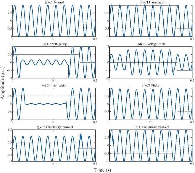
Figure 4 Normal waveform and seven single-disturbance waveforms (C0-C7).
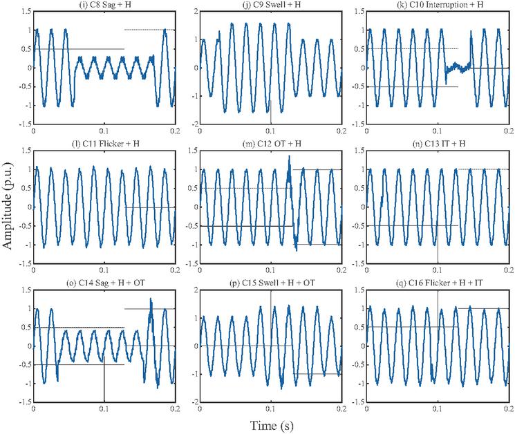
Figure 5 Nine compound-disturbance waveforms (C8-C16).
3 Disturbance Feature Extraction
3.1 Design of Feature Quantities
The S-transform is a multi-resolution analysis tool that integrates the advantages of both the Short-Time Fourier Transform (STFT) and the Wavelet Transform (WT), making it particularly suitable for time-frequency analysis of non-stationary signals [22]. As a linear transformation, the S-transform avoids the cross-term interference inherent in bilinear methods, thereby providing a reliable approach for analyzing power signals containing harmonics and various disturbances. Moreover, the S-transform yields a time-frequency spectrum that visually represents the energy distribution of the signal, which facilitates both manual inspection and feature extraction for machine learning applications. The mathematical definition of the S-transform is given as follows:
| (3) |
where is the Gaussian window function, expressed as:
| (4) |
The formula of the S-transform can be further simplified as:
| (5) |
A notable advantage of the S-transform is that its window width is inversely proportional to the square of the signal frequency, enabling adaptive adjustment of the Gaussian window’s scale. Specifically, narrower windows are used in high-frequency regions to capture rapid signal variations, whereas wider windows are applied in low-frequency regions to characterize long-term trends. This adaptability makes the S-transform particularly effective for capturing transient features in non-stationary signals and revealing the time-frequency coupling characteristics of power quality disturbances.
The S-transform produces a complex time-frequency matrix . Let and let denote the magnitude profile at the frequency bin nearest the 50 Hz fundamental. The five basic descriptors supplied by extract_features.m are defined below. They quantify RMS-event depth, waveform modulation, harmonic-band energy, and transient high-frequency activity rather than generic whole-matrix moments.
(1) F1: Normalized minimum fundamental amplitude ()
The reference is the temporal mean of . measures the deepest reduction of the fundamental profile and is therefore sensitive to voltage sag and interruption.
| (6) |
A smaller indicates a deeper and/or longer reduction of the fundamental component.
(2) F2: Normalized maximum fundamental amplitude ()
measures the largest elevation of the fundamental profile and provides the complementary descriptor for swell-dominated events.
| (7) |
Values above unity indicate an increase relative to the mean fundamental level.
(3) F3: Fundamental-profile correlation ()
The standardized fundamental profile is correlated with a standardized 50 Hz reference sequence. This coefficient captures the temporal regularity of the fundamental component and changes when modulation or abrupt events distort its time profile.
| (8) |
The coefficient is bounded to in the implementation.
(4) F4: Normalized mid-frequency energy ()
The 100–700 Hz band contains the principal field-calibrated 5th, 7th, 11th, and 13th harmonic components. is its squared-magnitude energy divided by total S-transform energy.
| (9) |
A larger indicates a stronger harmonic contribution relative to the complete spectrum.
(5) F5: Normalized high-frequency RMS amplitude ()
For , the RMS magnitude of the high-frequency S-transform region is normalized by the mean magnitude of the complete matrix. This descriptor responds to localized oscillatory and impulsive transient energy.
| (10) |
For numerical stability, the five descriptors are restricted to finite ranges before fold-wise standardization; the frequency boundaries remain fixed throughout the dataset.
These five descriptors form the original S-transform feature vector . The final physical branch additionally contains 51 enhanced S-transform statistics and 41 time-domain descriptors, allowing the tree ensemble to combine interpretable event depth, band-energy, transient-localization, and waveform-shape information.
3.2 Extraction of Feature Quantities
This study uses a two-channel CNN for automatic feature extraction from the S-transform. Channel 1 is the globally standardized log-magnitude map, which retains amplitude changes associated with sag, swell, and interruption. Channel 2 is the sample-wise standardized signed real component, which retains polarity, phase-related information, and temporal direction lost in a magnitude-only representation. Both channels have a spatial size of . The fusion model architecture is shown in Figure 6.
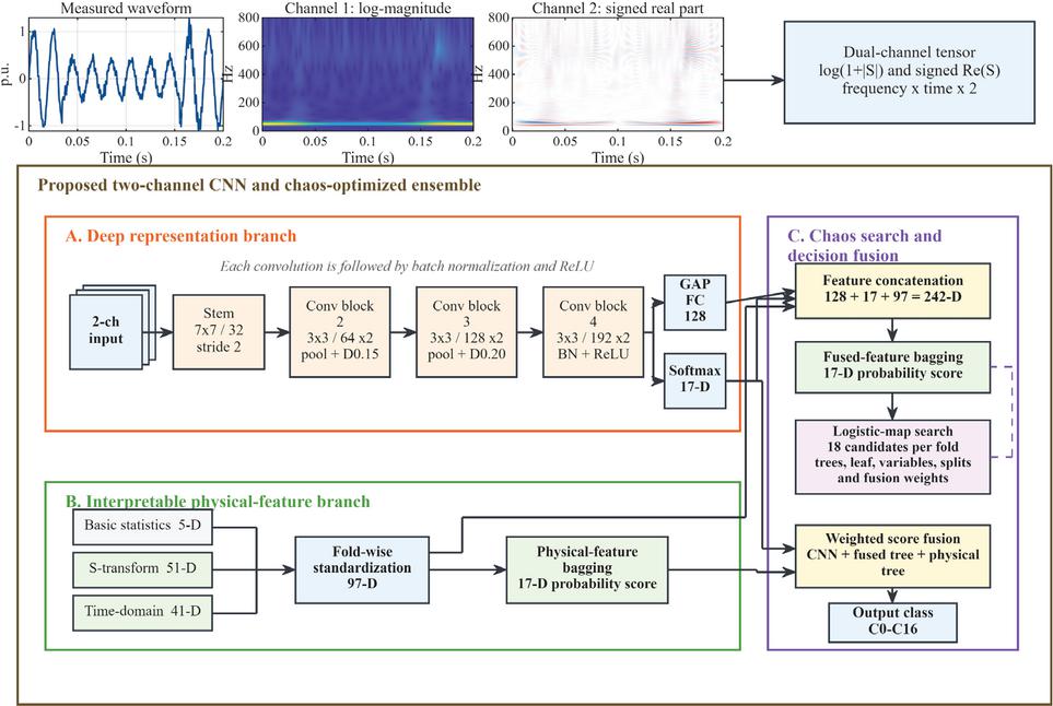
Figure 6 Architecture of the two-channel CNN and chaos-optimized probability-fusion model.
The paired S-transform channels are supplied directly to the CNN rather than converted to a single grayscale image. This design allows the network to learn energy-distribution patterns from the magnitude channel while using the signed channel to distinguish disturbances with similar magnitude spectra but different temporal or phase behavior.
The CNN backbone comprises a convolution with 32 channels and stride 2; two convolutions with 64 channels; two convolutions with 128 channels; and two convolutions with 192 channels. Batch normalization and ReLU activation follow each convolutional block, and max-pooling is applied after the 32-, 64-, and 128-channel stages. Global average pooling is followed by a 128-node fully connected layer, batch normalization, ReLU, and a 17 -node Softmax output layer. Dropout rates of 0.15, 0.20, and 0.35 are used after the 64-channel stage, 128-channel stage, and 128-node feature layer, respectively.
The network is trained with Adam for at most 90 epochs using a mini-batch size of 32, an initial learning rate of 0.001, piecewise learning-rate drops by a factor of 0.35 every 25 epochs, L2 regularization of , and a gradient threshold of 1. Within each outer training fold, 15% of the samples are reserved for validation; early stopping uses a patience of 12 and retains the network with minimum validation loss. Time-axis translations of 30 columns are used for training augmentation, and test-time averaging uses shifts of 24, 0, and 24 columns. The final tree input is a standardized 242-dimensional vector: 128 CNN activations, 17 CNN posterior probabilities, the five descriptors , 51 enhanced S-transform statistics, and 41 time-domain physical features. All normalization, early stopping, chaos search, and fusion-weight selection are determined exclusively from the outer training fold.
Table 3 Model parameter settings
| Module | Parameter | Setting Used in the Reported Experiments |
| Input | Two S-transform channels | (log-magnitude and signed real component) |
| CNN | Convolution channels | 32, 64, 128, and 192; seven convolutional layers |
| CNN | Activation/normalization | ReLU after batch normalization |
| CNN | Dropout | 0.15, 0.20, and 0.35 |
| Training | Adam | 90 epochs; batch 32; initial learning rate 0.001 |
| Training | Regularization/validation | |
| Tree input | Fused feature vector | ; 15% inner validation; patience 12 128 CNN + 17 posterior + 97 physical = 242 |
| Chaos search | Logistic map | r 4; 18 candidates per outer fold |
| Chaos search | Optimized variables | Tree count, leaf size, sampled features, split limit, and three fusion weights |
3.3 Ensemble Decision Tree with Chaos Optimization
For the conventional ensemble and the proposed chaos-optimized ensemble, the 242-dimensional fused vector is used as classifier input. The handcrafted-feature ablation uses a 56-dimensional vector comprising and the 51 enhanced S-transform statistics. Bagged decision trees are used in both ensemble variants, so their performance difference isolates chaos-based parameter selection and probability fusion rather than a change of tree family.
To achieve this, the construction process employs an information-theoretic approach, whereby entropy variation before and after splitting is used to evaluate the quality of each partition. Information Gain is adopted as the metric for assessing how much a feature contributes to data classification. It is defined as:
| (11) |
Where represents the information entropy of the dataset , measuring the uncertainty or disorder of the dataset. is the splitting feature, is a possible value of the feature, and is the subset corresponding to the value of feature . Thus, the decision tree model was constructed recursively by selecting the feature and splitting threshold that maximize information gain [25].
A Logistic-map chaos search is used to tune the ensemble and probability-level fusion on the internal validation subset only. For each outer fold, 18 chaotic candidates are evaluated. The search covers 220–520 trees, minimum leaf sizes of 1–11, feature-subsampling sizes from approximately the square root of the feature dimension to 85% of that dimension, and maximum split counts from 35% to 95% of the available fitting samples. Three nonnegative normalized weights combine the CNN posterior, the fused-feature tree posterior, and a separate physical-feature tree posterior. Candidate selection maximizes validation accuracy, with multiclass logarithmic loss used as the tie-breaker. The final selected configuration is then refitted on the complete outer training fold.
| (12) |
Where is the chaotic state at iteration . The Logistic control parameter is fixed at to obtain fully developed chaotic behavior, while fold-dependent initial values are used to avoid identical candidate sequences. Chaos generation is performed only during offline model selection.
The formal recognition experiment uses stratified five-fold cross-validation at 20 dB. Each fold contains 40 samples from every class; four folds are used for training and one for testing, and the procedure is repeated until every sample has served once as an outer test sample. Fold assignment is fixed by SourceID, so samples derived from the same operating condition cannot appear in both training and testing sets. Reported main accuracy is the mean and sample standard deviation across the five outer folds. Auxiliary sample-size, SNR, and mainstream-model studies use the same fixed source-isolated Fold 1 as an 80:20 holdout and are explicitly reported as single-holdout results rather than cross-validation means.
Computational complexity is separated into offline and online components. CNN training, fitting of candidate tree ensembles, and the 18-candidate chaos search are performed offline. For one online sample, the required operations are one S-transform, one CNN forward pass, and posterior evaluation of the selected tree ensembles. The CNN cost is dominated by the convolutional layers and scales with the sum of kernel area input channels output channels output-map area across layers; tree inference scales approximately with the number of selected trees multiplied by their average depth. The chaos sequence is not regenerated during online inference and therefore does not add repeated search latency to the deployed recognition stage.
4 Results and Discussion
4.1 PQD Identification Performance and Discussion
The main experiment uses a 2 kHz sampling frequency, a 0.2 s observation window, 20 dB SNR, 17 classes, and 200 samples per class (3,400 samples in total). Stratified source-isolated five-fold cross-validation gives 2,720 training samples and 680 test samples in each outer fold. The proposed method obtains 97.94%, 97.94%, 97.35%, 97.65%, and 97.06% on the five test folds. The 0.88-percentage-point range between the best and worst folds indicates that performance is not dominated by a favorable split and remains stable when complete source conditions are withheld.
Figure 7 compares the four required schemes fold by fold. Their mean accuracies are 86.56%, 96.21%, 96.88%, and 97.59%, respectively. The largest improvement is produced by replacing handcrafted S-transform descriptors with the two-channel CNN, confirming that magnitude and signed time-frequency maps capture compound-event structure that is not represented by low-dimensional statistics alone. Adding a conventional tree ensemble improves every fold, and chaos-optimized probability fusion again improves all five folds, with the largest gain occurring in Fold 3. The proposed method reaches 97.59% 0.38%, while its mean training-to-test gap is 1.92 percentage points. The small fold dispersion and moderate gap jointly indicate stable generalization under source-isolated evaluation.
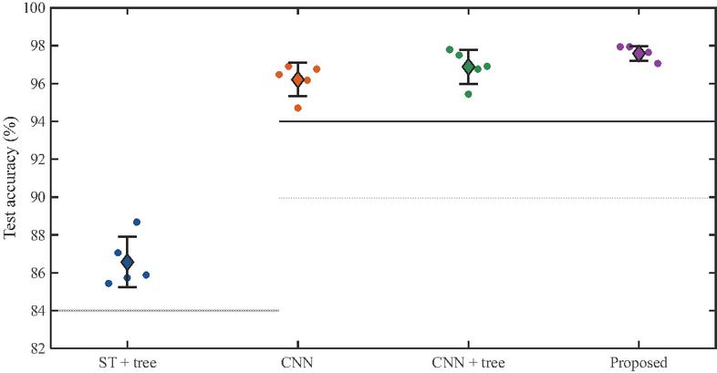
Figure 7 Five-fold classification accuracy of the four ablation schemes.
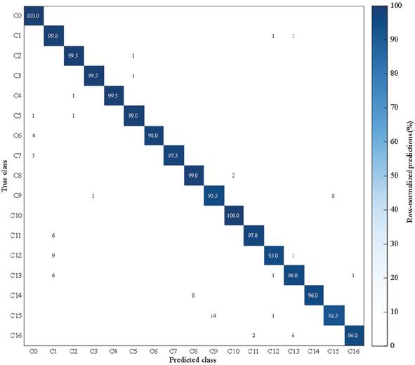
Figure 8 Aggregated test confusion matrix under five-fold cross-validation.
Figure 8 contains the aggregated 3,400 outer-test predictions. The dominant errors occur when a short or low-amplitude secondary event is superimposed on a stronger harmonic/RMS component. In particular, 14 C15 samples (voltage swell + harmonics + oscillatory transient) are assigned to C9 (voltage swell + harmonics), and 9 C12 samples (oscillatory transient + harmonics) are assigned to C1 (harmonics). Similarly, brief isolated transients account for four C6-to-C0 and five C7-to-C0 errors. These patterns are physically plausible because the transient occupies only 8-50 ms of the 0.2 s record and may approach the noise floor after exponential decay. Figure 9 provides the corresponding class-wise metrics: recall ranges from 92.50% to 100%, and 15 of the 17 classes achieve at least 95% recall. C1 has 99.0% recall but 90.41% precision because weak secondary events in several harmonic-bearing compound classes are reduced to their common harmonic signature. Importantly for the subsequent mitigation stage, these within-harmonic-group confusions preserve the harmonic-bearing decision.
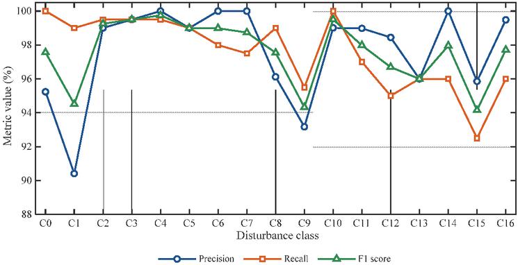
Figure 9 Per-class precision, recall, and F1 score from aggregated five-fold test predictions.
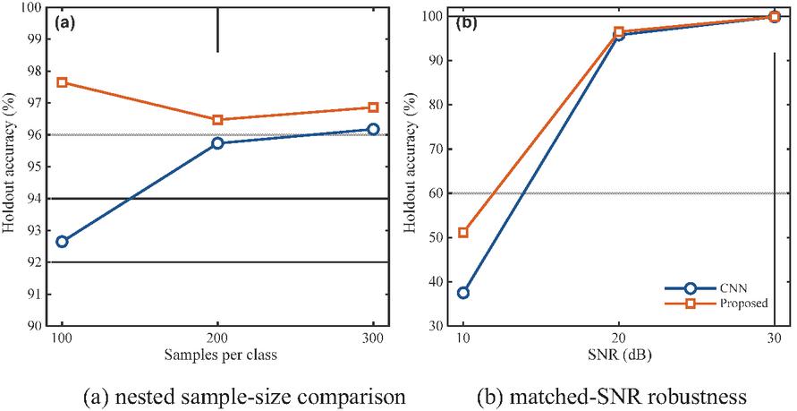
Figure 10 Fixed-holdout sensitivity analyses.
Figure 10(a) evaluates nested datasets of 100,200, and 300 samples per class on the same source-isolated holdout. The CNN-only accuracy rises from 92.65% to 96.18% as additional samples are included, whereas the proposed fusion remains in the narrow 96.47%–97.65% interval. The non-monotonic values of the proposed method (97.65%, 96.47%, and 96.86%) are expected for a single fixed holdout and should be interpreted as sensitivity bounds rather than a learning-curve trend. They nevertheless show that the physical and ensemble branches improve robustness in the lower-data regime. Figure 10(b) examines matched training and testing at 10, 20, and 30 dB. The proposed method improves the CNN by 13.68 percentage points at 10 dB and 0.74 points at 20 dB; both methods reach 99.85% at 30 dB. Thus, probability fusion is most useful before the high-SNR ceiling is reached, but it cannot fully recover the 2%–5% harmonic components when broadband noise dominates the short record at 10 dB.
Figure 11 compares representative classifiers on the same 20 dB source-isolated holdout, using an input suited to each model. RBF-SVM and random forest use the 97 physical/statistical features, GRU uses a compressed 24-channel S-transform sequence, and the CNN-based methods use the maps. The proposed model obtains 96.47%, compared with 90.44% for RBF-SVM, 94.26% for random forest, 65.44% for GRU, and 95.74% for the two-channel CNN. The 0.74-point gain over the identical CNN backbone isolates the benefit of adding optimized tree posteriors, while the random-forest result shows that physical features alone remain informative but do not capture the full time-frequency structure. The lower GRU result suggests that compressing the S-transform into a short sequence discards spatial detail needed to separate the mixed RMS, harmonic, and transient phenomena considered here.
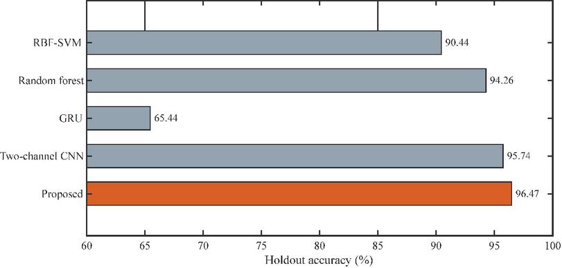
Figure 11 Comparison with mainstream classifiers under the fixed source-isolated holdout.
Table 4 summarizes the four-scheme ablation under the unified five-fold protocol. CNN representation learning contributes 9.65 percentage points over the handcrafted baseline. The conventional ensemble adds 0.68 points over CNN alone, and chaos-optimized three-way probability fusion adds a further 0.71 points over the conventional ensemble. Although the final increment is modest, it is positive in every outer fold and reduces the standard deviation from 0.91% to 0.38%. The contribution of chaos optimization is therefore expressed primarily as consistent fold-wise refinement and reduced split sensitivity, rather than as an isolated large accuracy jump.
Table 4 Ablation results under the unified five-fold main experiment
| Mean | |||
| Scheme Configuration | Accuracy (%) | Std. (%) | |
| 1 | S-transform features + decision-tree ensemble | 86.56 | 1.33 |
| 2 | CNN Softmax only | 96.21 | 0.88 |
| 3 | CNN features + conventional tree ensemble | 96.88 | 0.91 |
| 4 | CNN + chaos-optimized three-way tree fusion (proposed) | 97.59 | 0.38 |
Table 5 reports the numerical values underlying Figure 10(a). Because all capacities are nested subsets of one mother source pool, the comparison changes sample quantity without changing the disturbance-generation ranges. These single-holdout values are used only as data-scale sensitivity indicators; the principal recognition result remains the five-fold mean of 97.59% 0.38%.
Table 5 Sample-size sensitivity on a fixed source-isolated holdout set (20 dB)
| Samples Per Class | Total Samples | CNN Accuracy (%) | Proposed Accuracy (%) |
| 100 | 1,700 | 92.65 | 97.65 |
| 200 | 3,400 | 95.74 | 96.47 |
| 300 | 5,100 | 96.18 | 96.86 |
Table 6 Comparison with mainstream algorithms on the fixed source-isolated holdout set (20 dB, 200 samples per class)
| Holdout | ||
| Algorithm | Input/Model Description | Accuracy (%) |
| RBF-SVM | 97 physical and S-transform statistical features | 90.44 |
| Random forest | 97 physical and S-transform statistical features | 94.26 |
| GRU | 24-channel compressed S-transform sequence | 65.44 |
| Two-channel CNN | S-transform input | 95.74 |
| Proposed method | CNN + chaos-optimized tree probability fusion | 96.47 |
Table 6 complements the ablation by comparing established model families under the same holdout and SNR. The proposed method exceeds RBF-SVM, random forest, GRU, and the two-channel CNN by 6.03, 2.21, 31.03, and 0.74 percentage points, respectively. Since the CNN and proposed method share the same image input and backbone, their difference is the most direct evidence for the added value of the optimized ensemble. The other comparisons show the consequence of using model-appropriate statistical or sequential representations and are interpreted as broader reference baselines.
Taken together, the source-isolated five-fold result, class-level error structure, nested sample-size study, matched-SNR test, and mainstream-model comparison show that the proposed improvement is repeatable across folds and is not explained by a single favorable split. The remaining errors are concentrated in weak secondary transients, which also defines the principal recognition boundary for short records at severe noise levels.
4.2 Diagnosis-Guided Harmonic Mitigation and Engineering Interpretation
The purpose of this stage is to convert the recognition result into information that can support harmonic-mitigation design. The 17-class output is first mapped to a harmonic-bearing decision: C1 and C8-C16 enter the HAPF assessment branch, whereas C0 and C2-C7 remain disturbance records for other mitigation measures. Aggregating the five-fold confusion matrix according to this mapping gives 1,999 correct harmonic decisions, one missed harmonic case, no false harmonic decision, and 1,400 correct non-harmonic decisions. The resulting 99.97% decision accuracy, 99.95% sensitivity, and 100% precision show that most class-level confusions in Figures 8 and 9 occur within the same mitigation group. Consequently, the classifier can remain useful for strategy selection even when a weak secondary disturbance is not assigned its exact compound label. Figure 12 illustrates the complete diagnosis-guided harmonic mitigation workflow built on the above classification strategy. It covers the full implementation chain from field PCC waveform acquisition, compound disturbance identification, harmonic-bearing decision, order-resolved spectral decomposition, to the parameter configuration and performance verification of the equivalent HAPF model, and intuitively demonstrates how the diagnostic output is mapped to the hybrid filtering scheme.
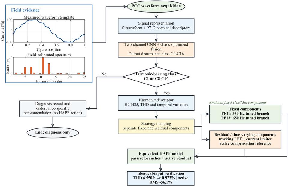
Figure 12 Diagnosis-guided identification and harmonic-mitigation workflow.
For a harmonic-bearing case, the diagnostic front end provides the descriptor . This vector supplies three quantities required by the equivalent HAPF design: the target harmonic orders, the passive/active current-sharing ratio, and the active-branch current rating. The field spectrum identifies the 11th and 13th components as dominant stationary targets, so they are assigned to single-tuned passive branches. At the 0.4 kV equivalent bus, with and with produce resonances at 550 and 650 Hz. The APF tracks the remaining 2nd-25th harmonic reference with a 4 kHz equivalent bandwidth, and the residual spectrum determines a 36 A RMS active rating. The model uses a 1,000 A phase current base, a 20 kHz sampling frequency, a 0.30 s interval, filter insertion at 0.04 s, and a 0.90 passive capture coefficient. This equivalent model resolves harmonic-current allocation and capacity requirements; converter switching ripple, semiconductor losses, and controller implementation are outside its present scope.
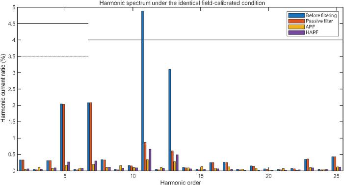
Figure 13 Harmonic-spectrum comparison.
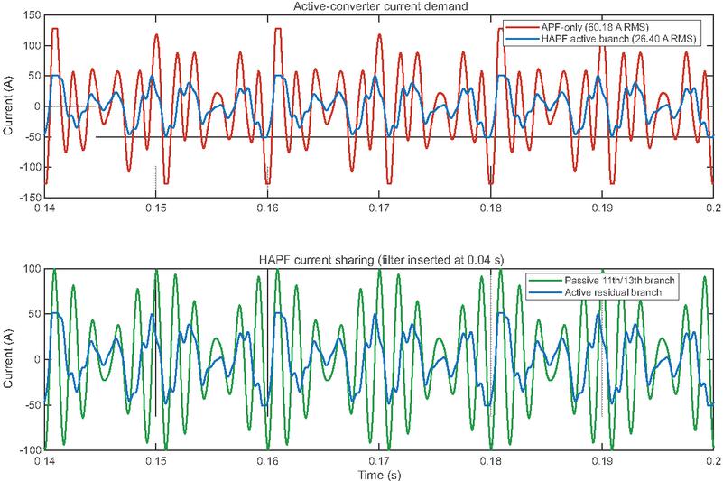
Figure 14 Equivalent HAPF simulation results under the identical field-calibrated condition.
Figures 13, 14 and Table 7 compare passive-filter, APF-only, and HAPF operation using the same reconstructed PCC waveform, time window, and harmonic estimator. The passive branches reduce the dominant 11th and 13th components and lower THD from 6.550% to 3.241%, but the remaining 5th, 7th, and non-target components prevent the passive-only scheme from achieving the desired residual distortion. APF-only compensation reaches 0.667% THD but requires 60.18 A RMS of active current. The HAPF reaches 0.973% THD with 26.40 A RMS of active current, a 56.1% reduction in active-converter demand. The small 0.306-percentage-point THD increase relative to APF-only operation is therefore exchanged for a substantial reduction in converter current capacity while maintaining THD below 1%. This current-sharing trade-off, rather than minimum THD alone, is the principal engineering benefit of using the diagnosis-derived dominant orders to configure the hybrid topology.
Table 7 Equivalent filtering performance under the identical field-calibrated condition
| Metric | Before Filtering | Passive Filter | APF | HAPF |
| 5th harmonic (%) | 2.045 | 2.041 | 0.172 | 0.278 |
| 7th harmonic (%) | 2.088 | 2.082 | 0.204 | 0.302 |
| 11th harmonic (%) | 4.885 | 0.877 | 0.340 | 0.665 |
| 13th harmonic (%) | 3.103 | 0.619 | 0.287 | 0.493 |
| THD (%) | 6.550 | 3.241 | 0.667 | 0.973 |
| Active current (A RMS) | 0 | 0 | 60.18 | 26.40 |
The mitigation study completes the harmonic-bearing branch of the proposed workflow. Recognition determines whether harmonic treatment is relevant, the extracted spectrum selects the fixed passive targets, and the residual spectrum determines the active compensation burden. The resulting comparison demonstrates that diagnostic information can support both filter-parameter matching and converter-capacity reduction. The present equivalent simulation establishes this design-level relationship and provides a defined basis for subsequent hardware-in-the-loop and field validation.
5 Conclusion
This paper developed a field-calibrated workflow for identifying compound PQDs and using the resulting diagnosis to parameterize harmonic mitigation in a PV-rich distribution network. IEEE Std 1159-2019-constrained ranges provide disturbance diversity, while the measured Cable9 spectrum anchors the harmonic component. The two-channel S-transform representation preserves complementary magnitude and signed information, and the fused physical branch retains interpretable event-depth, band-energy, and transient-localization cues.
Under 20 dB SNR, 200 samples per class, and source-isolated five-fold cross-validation, the proposed method achieves 97.59% 0.38% accuracy. The four ablation means of 86.56%, 96.21%, 96.88%, and 97.59% show that CNN representation learning provides the main gain, while the chaos-optimized fusion supplies a smaller but fold-consistent improvement and lowers split sensitivity. Error analysis further shows that the remaining ambiguity is concentrated in weak secondary transients, especially under the 10 dB severe-noise condition.
Mapping the 17 labels to harmonic-bearing and non-harmonic groups gives 99.97% decision accuracy, indicating that most residual class confusions do not alter the mitigation branch. Under the field-calibrated equivalent condition, diagnosis-guided allocation of the 11th and 13th components to passive branches and the residual spectrum to the active branch reduces THD from 6.550% to 0.973%. Compared with APF-only operation, the HAPF reduces active-converter RMS current by 56.1% while maintaining sub-1% THD.
Overall, the results demonstrate that compound-disturbance diagnosis can contribute not only a class label but also actionable spectral information for filter targeting and capacity allocation. Future work will extend the equivalent model to hardware-in-the-loop and field tests, with emphasis on controller delay, switching effects, parameter drift, and end-to-end implementation under changing operating conditions.
Potential Conflicts of Interest
The author declares that there is no potential conflict of interest.
Funding Information
This paper was supported by the Natural Science Foundation of Fujian Province under the project “Research on Key Technologies of Intelligent Monitoring Considering Distributed Photovoltaic Power” (2022J05284).
Research Involving Human Participants And/Or Animals
Not Applicable.
Informed Consent
The author unanimously agreed to the revision and publication of the manuscript.
Data Availability
Not Applicable.
Ethics Statement
Not applicable. This study uses field electrical measurements, synthetic disturbance signals, and simulation models and does not involve human participants, animals, or personal data.
References
[1] Q. A. Qawaqneh, “Impact of 11kV Capacitor Bank Switching at Distribution Power Network from Power Quality Perspective,” 2020 19th International Conference on Harmonics and Quality of Power (ICHQP), Dubai, United Arab Emirates, 2020, pp. 1–6, doi: 10.1109/ICHQP46026.2020.9177911.
[2] A. Ballaji and R. Dash, “A Comprehensive Review on Latest State of the Art Practices in MPPT Algorithm”, Distributed Generation & Alternative Energy Journal, vol. 38, no. 03, pp. 875–906, Mar. 2023. https://doi.org/10.13052/dgaej2156-3306.3837.
[3] A. Bayu, D. Anteneh, and B. Khan, “Grid Integration of Hybrid Energy System for Distribution Network,” Distributed Generation & Alternative Energy Journal, vol. 37, no. 3, pp. 667–675, 12/07 2021. https://doi.org/10.13052/dgaej2156-3306.3738.
[4] S. Sampurna, A. Ranjan and G. Singh, “Performance comparison of feature extraction techniques for power quality disturbances,” 2023 Second IEEE International Conference on Measurement, Instrumentation, Control and Automation (ICMICA), Kurukshetra, India, 2024, pp. 1–6, doi: 10.1109/ICMICA61068.2024.10732115.
[5] K. Sekar, S. Kumar. S and K. K, “Power Quality Disturbance Detection using Machine Learning Algorithm,” 2020 IEEE International Conference on Advances and Developments in Electrical and Electronics Engineering (ICADEE), Coimbatore, India, 2020, pp. 1–5, doi: 10.1109/ICADEE51157.2020.9368939.
[6] Z. Chen, H. Zhang, H. Sun and B. Gao, “Power quality comprehensive evaluation method of regional distribution network based on random forest,” 2024 4th International Conference on New Energy and Power Engineering (ICNEPE), Guangzhou, China, 2024, pp. 1031–1037, doi: 10.1109/ICNEPE64067.2024.10860332.
[7] J. He, Y. Chen, W. Zheng, J. Zhang and T. Zhao, “Classification of power quality disturbances using Kolmogorov-Arnold Network,” 2024 4th International Conference on Intelligent Power and Systems (ICIPS), Yichang, China, 2024, pp. 1001–1005, doi: 10.1109/ICIPS64173.2024.10899817.
[8] S. R. K. Joga, S. S. M. N. Surisetti, S. Karri, S. Jalaluddin, K. Madhu and J. Shiva, “Detection and Classification of Changes in Voltage Magnitude During Various Power Quality Disturbances,” 2023 4th International Conference for Emerging Technology (INCET), Belgaum, India, 2023, pp. 1–6, doi: 10.1109/INCET57972.2023.10170211.
[9] Z. Ren and Y. Ye, “Classification of Power Quality Disturbances Based on Multi-domain Parallel Feature Extraction and Optimization Strategy,” 2023 35th Chinese Control and Decision Conference (CCDC), Yichang, China, 2023, pp. 1050–1055, doi: 10.1109/CCDC58219.2023.10326531.
[10] H. He, J. Wei, G. Li, H. Cao and K. Sun, “Feature Extraction Method of Power Quality Disturbances Based on PSO and VMD,” 2024 IEEE 7th Information Technology, Networking, Electronic and Automation Control Conference (ITNEC), Chongqing, China, 2024, pp. 1628–1632, doi: 10.1109/ITNEC60942.2024.10733033.
[11] H. Shao, R. Henriques, H. Morais and E. Tedeschi, “Automatic Power Quality Disturbance Feature Extraction Using Fast Iterative Filtering,” 2024 21st International Conference on Harmonics and Quality of Power (ICHQP), Chengdu, China, 2024, pp. 660–665, doi: 10.1109/ICHQP61174.2024.10768829.
[12] H. Zhang et al., “Disturbance Identification of Power Quality Based on Markov Transition Field and Deep Residual Network,” 2023 3rd International Conference on Energy Engineering and Power Systems (EEPS), Dali, China, 2023, pp. 539–543, doi: 10.1109/EEPS58791.2023.10256704.
[13] S. Sampurna, A. Ranjan and G. Singh, “Performance comparison of feature extraction techniques for power quality disturbances,” 2023 Second IEEE International Conference on Measurement, Instrumentation, Control and Automation (ICMICA), Kurukshetra, India, 2024, pp. 1–6, doi: 10.1109/ICMICA61068.2024.10732115.
[14] X. Wang, J. Tian, Q. Wang and Y. Yu, “Significant Target-Guided Feature Extraction Algorithm Based on Optimized Superpoint,” 2024 6th International Conference on Communications, Information System and Computer Engineering (CISCE), Guangzhou, China, 2024, pp. 349–353, doi: 10.1109/CISCE62493.2024.10653190.
[15] H. Meena, H. K. Meena and D. Saxena, “Classification of power quality disturbances with DWT based effective feature extraction,” 2021 4th International Conference on Recent Trends in Computer Science and Technology (ICRTCST), Jamshedpur, India, 2022, pp. 314–320, doi: 10.1109/ICRTCST54752.2022.9781895.
[16] J. Kumar, S. Ansari, O. H. Gupta, A. K. Singh, and V. K. Sood, “An Adaptive Filter Algorithm Based on Hyperbolic Tangent Function for Power Quality Enhancement in Distribution Network”, Distributed Generation & Alternative Energy Journal, vol. 40, no. 01, pp. 29–62, Apr. 2025. https://doi.org/10.13052/dgaej2156-3306.4012.
[17] W. Yong, P. Heping, M. Wenxiong, L. Le and X. Zhong, “A Local Density Clustering Based Method for Disturbance Source Identification of Power quality in Distribution Systems,” 2021 International Conference on Power System Technology (POWERCON), Haikou, China, 2021, pp. 1980–1985, doi: 10.1109/POWERCON53785.2021.9697635.
[18] M. Liao and H. Liu, “Power Quality Disturbance Identification Based on Optimized VMD and CNN-BiGRU,” 2024 21st International Conference on Harmonics and Quality of Power (ICHQP), Chengdu, China, 2024, pp. 576–581, doi: 10.1109/ICHQP61174.2024.10768693.
[19] R. Kumar, R. Kumar, S. Marwaha and B. Singh, “S-Transform Based Detection of Multiple and Multistage Power Quality Disturbances,” 2020 IEEE 9th Power India International Conference (PIICON), Sonepat, India, 2020, pp. 1–5, doi: 10.1109/PIICON49524.2020.9112945.
[20] F. Guo, J. Li, X. Xu, Y. Zhu, X. Luo and W. Qian, “Classification of Transient Power Quality Disturbances Based on Digital Image Processing Techniques,” 2023 8th International Conference on Power and Renewable Energy (ICPRE), Shanghai, China, 2023, pp. 492–498, doi: 10.1109/ICPRE59655.2023.10353758.
[21] IEEE, “IEEE Recommended Practice for Monitoring Electric Power Quality,” IEEE Std 1159-2019 (Revision of IEEE Std 1159-2009), pp. 1–98, Aug. 2019, doi: 10.1109/IEEESTD.2019.8796486.
[22] Y. Zhao, Z. Zou, L. Wu and Y. Li, “Frequency Detection Algorithm for Frequency Diversity Signal Based on STFT,” 2015 Fifth International Conference on Instrumentation and Measurement, Computer, Communication and Control (IMCCC), Qinhuangdao, China, 2015, pp. 790–793, doi: 10.1109/IMCCC.2015.173.
[23] W. Deng, D. Xu, Y. Xu and M. Li, “Detection and Classification of Power Quality Disturbances Using Variational Mode Decomposition and Convolutional Neural Networks,” 2021 IEEE 11th Annual Computing and Communication Workshop and Conference (CCWC), NV, USA, 2021, pp. 1514–1518, doi: 10.1109/CCWC51732.2021.9376031.
[24] C. Zhou, Z. Shao, F. Chen and Y. Zhang, “Classification of Power Quality Disturbance Signals Based on Weighting Random Forest,” 2022 7th Asia Conference on Power and Electrical Engineering (ACPEE), Hangzhou, China, 2022, pp. 2052–2056, doi: 10.1109/ACPEE53904.2022.9783958.
[25] I. Jahan, F. Mohamed, V. Blazek, L. Prokop, S. Misak and V. Snasel, “Power Quality Parameters Forecasting Based on SOM Maps with KNN Algorithm and Decision Tree,” 2023 23rd International Scientific Conference on Electric Power Engineering (EPE), Brno, Czech Republic, 2023, pp. 1–6, doi: 10.1109/EPE58302.2023.10149269.
[26] X. Bu, Q. Zhang and G. Zhao, “A Power Supply Service Quality Analysis Method Based on Information Entropy Decision Tree Algorithm,” 2023 Global Conference on Information Technologies and Communications (GCITC), Bangalore, India, 2023, pp. 1–5, doi: 10.1109/GCITC60406.2023.10426066.
[27] A. Asheibi, A. Khalil and Z. Rajab, “Predicting Power Quality Disturbance Events from Weather Conditions Using Gaussian Mixture Model and Decision Tree,” 2023 10th International Conference on Electrical and Electronics Engineering (ICEEE), Istanbul, Turkiye, 2023, pp. 469–474, doi: 10.1109/ICEEE59925.2023.00091.
Biographies

Zhiquan Liu graduated from Xiamen University of Technology in 2022. He is currently studying for a master’s degree at Xiamen University of Technology. The main research directions include power quality detection and analysis, harmonic control.

Jun Su obtained a Bachelor’s degree in Electrical Engineering at Staffordshire University in 2012, followed by a Master’s degree in Electrical Energy Systems from Cardiff University in 2014. From October 2017 to December 2020, pursued PhD in Electrical Engineering at Auckland University of Technology, New Zealand. Since July 2021, began teaching at the School of Electrical Engineering and Automation at Xiamen University of Technology. Primary research interests include electric vehicles charging strategy, renewable energy generation systems, intelligent distribution networks.

Chaolong Tang graduated from Xiamen University of Technology in 2022. He is currently studying for a master’s degree at Xiamen University of Technology. The main research directions include photovoltaic power prediction.

Yaoyi Wu graduated from Xiamen University of Technology in 2023. He is currently studying for a master’s degree at Xiamen University of Technology. The main research directions include electric power system intelligent operation and maintenance.
Distributed Generation & Alternative Energy Journal, Vol. 41_5, 1453–1484
doi: 10.13052/dgaej2156-3306.4159
© 2026 River Publishers