Multi-site Wind Energy Prediction System Based on Power Decomposition and Deep Model Integration

Zhiyi Xie, Zhanjun Tang^* and Wenbang Zhang

Kunming University of Science and Technology, Chenggong 650500, Kunming, China
E-mail: xie1138802610@163.com
*Corresponding Author

Received 13 April 2026; Accepted 28 May 2026

Abstract

To address the limitations of existing wind power forecasting methods in mixed-frequency signal modeling, multi-site spatial correlation capture, and single-model generalization, this paper proposes a multi-site wind power forecasting system based on power decomposition and deep model ensemble. The system applies Variational Mode Decomposition (VMD) to separate raw power sequences into high-frequency and low-frequency components, each directed into a structurally symmetric dual-branch framework. Within each branch, three heterogeneous sub-models – ConvGAT-LSTM, Spectral Transformer, and TCN – operate in parallel; branch outputs are aggregated by simple averaging and linearly combined into a base prediction, which is subsequently refined by an XGBoost residual correction layer. Experiments on six Chinese wind farm datasets demonstrate that the proposed system achieves an average RMSE of $0.1065\pm 0.0021$ and ${\mathrm{R}}^2$ of $0.8335\pm 0.0167$ at the 24-step forecast horizon, improving over the state-of-the-art baseline TCOAT by 1.4% and 0.5%, respectively. The VMD module alone contributes an 11.6% RMSE reduction, and the system reduces local RMSE during ramp events at Site 6 by 34.9% relative to the baseline. Ablation experiments and statistical significance tests ($\mathrm{p}<0.05$, Cohen’s $\mathrm{d}>0.82$) confirm that each module contributes meaningfully to overall performance.

Keywords: Wind power forecasting, variational mode decomposition, deep model ensemble, graph attention network, temporal convolutional network, residual correction.

1 Introduction

In 2023, the global installed wind power capacity exceeded 1,000 GW, with a growth rate of (15%), yet the annual average wind curtailment rate of grid dispatching agencies in China’s northwest region still exceeded (11%). The fundamental reason for this loss lies in insufficient prediction accuracy rather than a lack of physical resources (Zhang et al., 2024b). At the turbine level, wind speed prediction errors are nonlinearly amplified into power output deviations through the cubic relationship in the wind power equation,

$$\mathrm{P}=\frac{1}{2}\rho {\mathrm{Av}}^3{\mathrm{C}}_{\mathrm{p}}$$

(1)

meaning that minor disturbances in meteorological uncertainty can be transformed into substantial risks in power dispatching. Multi-site wind farms further exacerbate this challenge: adjacent sites with a geographical distance of only 20 kilometers may exhibit decoupled power fluctuations driven by mesoscale atmospheric vortices, requiring prediction systems to not only analyze local turbulence characteristics but also capture spatial coherence structures between sites. The currently widely adopted standalone deployment scheme for single sites completely ignores the cross-site dependencies within wind farm clusters, precisely missing the most valuable spatial correlation information during critical periods when power ramp-up events are most intense and grid balance pressure is greatest.

The original wind power time series exhibits significant spectral heterogeneity: low-frequency components with periods exceeding 6 hours reflect the evolution of weather-scale systems and demonstrate relatively strong predictability, while sub-hourly high-frequency residuals originate from boundary layer turbulence governed by chaotic dynamics. The standard LSTM architecture processes this mixed-frequency signal through a single recurrent pathway, forcing hidden states to simultaneously encode trend-level memory and noise-level responses-two objectives that generate opposing gradient pressures during backpropagation (Li et al., 2019). Although CNN-based methods excel in local pattern extraction, uniform convolution kernels applied across the full time spectrum suppress real noise while attenuating valuable high-frequency transient components. Transformer models with long-range dependency modeling capabilities demonstrate quadratic growth in computational complexity of their self-attention mechanisms with sequence length, and exhibit training instability when processing short-term historical records (12–24 months) from newly operational sites (Wang et al., 2024a). Graph neural network approaches like ST-GNN capture inter-site geographic distance correlations through fixed adjacency matrices, yet wind power coherence is fundamentally determined by atmospheric stability states that dynamically vary with seasonal and diurnal cycles. Static graph topologies fail to characterize this time-varying dependency relationship.

The system proposed in this paper fundamentally differs from prior works in four key technical contributions. During the signal decomposition preprocessing phase, VMD separates historical power data from each station into high-frequency and low-frequency sub-sequences, directing each component to dedicated modeling branches to ensure the architecture’s inductive bias aligns with the statistical characteristics of corresponding frequency bands. Within each branch, three structurally heterogeneous sub-models operate in parallel: ConvGAT-LSTM processes exogenous meteorological features through an attention-enhanced frequency-domain module, which integrates cross-site multi-head attention networks with power historical data. The Spectral Transformer embeds FFT-derived amplitude, phase, mean (d $=$ 1,2,4), and standard deviation features into a Transformer encoder stack, with predictions generated by a residual-connected MLP curve predictor. The TCN, featuring exponential cavity rate growth, captures multi-scale temporal patterns via causal convolution without recurrent bottlenecks. Branch-level predictions undergo simple mean aggregation, with linear fusion of outputs from both branches forming the base prediction. The variance-weighted mechanism within ConvGAT-LSTM dynamically adjusts contribution weights of parallel LSTM units based on output statistics to estimate prediction uncertainty. Finally, a XGBoost meta-learner trained on residuals between base predictions and actual values applies structural corrections to address systematic biases unresolvable by neural network components.

2 Related Work

2.1 Deep Learning-Based Wind Power Prediction Method

The long-term and short-term memory networks selectively retain or forget historical information through gate mechanisms, with their hidden state update rule being:

$${\mathrm{f}}_{\mathrm{t}}=\sigma ({\mathrm{W}}_{\mathrm{f}}\cdot [{\mathrm{h}}_{\mathrm{t}-1},{\mathrm{x}}_{\mathrm{t}}]+{\mathrm{b}}_{\mathrm{f}})$$
$${\mathrm{i}}_{\mathrm{t}}=\sigma ({\mathrm{W}}_{\mathrm{i}}\cdot [{\mathrm{h}}_{\mathrm{t}-1},{\mathrm{x}}_{\mathrm{t}}]+{\mathrm{b}}_{\mathrm{i}})$$
$${\mathrm{C}}_{\mathrm{t}}={\mathrm{f}}_{\mathrm{t}}\odot {\mathrm{C}}_{\mathrm{t}-1}+{\mathrm{i}}_{\mathrm{t}}\odot {\widehat{\mathrm{C}}}_{\mathrm{t}}$$	(2)

Among ${\mathrm{f}}_{\mathrm{t}}$, ${\mathrm{i}}_{\mathrm{t}}$, ${\mathrm{C}}_{\mathrm{t}}$, ${\mathrm{W}}_{\mathrm{f}}$, ${\mathrm{W}}_{\mathrm{i}}$, and $\sigma$, ${\mathrm{f}}_{\mathrm{t}}$ outputs for the forgetting gate, ${\mathrm{i}}_{\mathrm{t}}$ outputs for the input gate, ${\mathrm{C}}_{\mathrm{t}}$ represents the unit state, ${\mathrm{W}}_{\mathrm{f}}$ and ${\mathrm{W}}_{\mathrm{i}}$ correspond to the weight matrix, and $\sigma$ uses the Sigmoid activation function, while $\odot$ denotes element-wise product. Li et al. (2019) validated the predictive capability of standard LSTM on 6 China wind farm datasets, with an average RMSE of 0.1151. However, this architecture exhibited significant phase lag when processing sub-hourly high-frequency fluctuations, as a single hidden state cannot simultaneously maintain long-term memory of low-frequency trends and rapid response to high-frequency transients. To address this limitation, Zheng and Li (2023) combined the local feature extraction capability of CNN with the sequence modeling ability of LSTM. The CNN layer performs operations on the input feature map using the width of the convolution kernel:

$${\mathrm{Z}}_{\mathrm{j}}=\mathrm{ReLU}\left(\sum _{\mathrm{f}=1}^{\mathrm{F}}{\mathrm{W}}_{\mathrm{j},\mathrm{f}}\ast {\mathrm{X}}_{\mathrm{f}}+{\mathrm{b}}_{\mathrm{j}}\right)$$

(3)

The notation $\ast$ denotes a one-dimensional convolution, where ${\mathrm{W}}_{\mathrm{j},\mathrm{f}}$ denotes the convolution kernel of the $\mathrm{j}$-th filter applied to the $\mathrm{f}$-th feature channel, and ${\mathrm{Z}}_{\mathrm{j}}$ denotes the corresponding feature map. This hybrid architecture achieves approximately 10% lower average MAE and 8.3% higher ${\mathrm{R}}^2$ than pure LSTM models, yet its uniform receptive field of convolution kernels lacks adaptability for wind speed ramping events spanning different time scales. After introducing the self-attention mechanism in the Transformer architecture, Wang et al. (2024a) reported a 0.79 prediction accuracy on a 72-step time domain, surpassing the LSTM+CNN combination with equivalent parameter sizes. However, the Transformer architecture requires approximately 2.3 times more training data than the latter, demonstrating a significant sample efficiency disadvantage in short-historical scenarios of newly operational wind farms.

Table 1 Comparison of performance of major deep learning prediction methods (24-step prediction time domain)

Method	Average RMSE	Average MAE	${\mathrm{R}}^2$	Parameter (K)
LSTM (Li et al., 2019)	0.1151	0.0760	0.8080	41.2
CNN+Attention (Xiong et al., 2022)	0.1118	0.0728	0.8194	38.7
LSTM+CNN (Wu et al., 2021)	0.1344	0.0833	0.7211	55.3
LSTM+CNN+Attention (Wan et al., 2023)	0.1225	0.0797	0.7842	62.1
Transformer (Wang et al., 2024a)	0.1109	0.0715	0.8267	124.6
Data source: Experimental results compiled by Sarkar et al. (2026), with the test set being the China six-site wind farm dataset.

2.2 Time Series Decomposition Method

Variational mode decomposition (VMD) decomposes the original $\mathrm{x}(\mathrm{t})\mathrm{K}$ signal into a set of eigenmode functions (IMFs) by solving the following constrained optimization problem:

$$\underset{\{{\mathrm{u}}_{\mathrm{k}}\},\{{\omega }_{\mathrm{k}}\}}{\min }\left\{\sum _{\mathrm{k}=1}^{\mathrm{K}}{\Vert {\partial }_{\mathrm{t}}\left[\left(\delta (\mathrm{t})+\frac{\mathrm{j}}{\pi \mathrm{t}}\right)\ast {\mathrm{u}}_{\mathrm{k}}(\mathrm{t})\right]{\mathrm{e}}^{-\mathrm{j}{\omega }_{\mathrm{k}}\mathrm{t}}\Vert }_2^2\right\}$$
$$\mathrm{s}.\mathrm{t}.\sum _{\mathrm{k}=1}^{\mathrm{K}}{\mathrm{u}}_{\mathrm{k}}(\mathrm{t})=\mathrm{x}(\mathrm{t})$$	(4)

Here, ${\mathrm{u}}_{\mathrm{k}}(\mathrm{t})$ represents the $\mathrm{k}$-th modal component, with ${\omega }_{\mathrm{k}}$ the corresponding center frequency and $\delta (\mathrm{t})$ the Dirac distribution, where $\ast$ denotes the convolution operation. Unlike the recursive screening mechanism of Empirical Mode Decomposition (EMD), VMD employs Alternating Directional Multiplicative Method (ADMM) to solve each mode in parallel within the frequency domain, fundamentally avoiding the inherent modal aliasing problem of EMD. Yang et al. (2023) applied VMD to decompose each IMF component into independent predictive models, achieving 14.7% lower Root Mean Square Error (RMSE) than direct prediction of the original sequence at highly variable sites with power fluctuation standard deviation exceeding 150 MW. Fast Fourier Transform (FFT) provides another frequency-domain decomposition approach, with its discrete form expressed as:

$$\mathrm{X}[\mathrm{k}]=\sum _{\mathrm{n}=0}^{\mathrm{N}-1}\mathrm{x}[\mathrm{n}]\cdot {\mathrm{e}}^{-\mathrm{j2}\pi \mathrm{kn}/\mathrm{N}},\mathrm{k}=0,1,\mathrm{\dots },N-1.$$

(5)

The complex number $\mathrm{X}[\mathrm{k}]$ represents the $\mathrm{k}$-th frequency component, where $\mathrm{N}$ is the sequence length and $\mathrm{x}[\mathrm{n}]$ is the observed value at the $\mathrm{n}$-th time step. The computational complexity $\mathrm{O}(\mathrm{N}\log \mathrm{N})$ of FFT is significantly lower than that of VMD’s iterative solution cancellation, but its fixed-frequency resolution is less effective in extracting transient characteristics from non-stationary wind power sequences compared to VMD.

Table 2 Comparison of characteristics of main decomposition methods in wind power forecasting

				Predicted
Decomposition	Computation	Modal	Nonstationary	RMSE
Method	Complexity	Aliasing	Adaptability	Improvement
EMD	$O(N\log N)$	Exist	Secondary	8.2
VMD	$O(KN\log N)$	Not have	Strong	14.7
FFT	$O(N\log N)$	Not have	Weak	6.5
Wavelet decomposition	$O(N)$	Light	Stronger	11.3
Data source: Experimental data compiled from Yang et al. (2023) and Sarkar et al. (2026), with the baseline being the undecayed direct prediction results.

2.3 Integrated Learning and Meta-learning Methods

The Stacking framework utilizes outputs from multiple base learners as input features for meta-learners. Let the set of base learners be defined as ${\mathrm{f}}_1,{\mathrm{f}}_2,\mathrm{\dots },{\mathrm{f}}_{\mathrm{M}}$, where each model’s prediction output for sample ${\mathrm{x}}_{\mathrm{i}}$ forms the meta-feature vector.

$${\mathrm{X}}_{\mathrm{i}}={[{\mathrm{f}}_1({\mathrm{x}}_{\mathrm{i}}),{\mathrm{f}}_2({\mathrm{x}}_{\mathrm{i}}),\mathrm{\dots },{\mathrm{f}}_{\mathrm{M}}({\mathrm{x}}_{\mathrm{i}})]}^{\top }\in {ℝ}^{\mathrm{M}}.$$

(6)

The meta-learning framework then learns the optimal combination mapping ${\widehat{\mathrm{y}}}_{\mathrm{i}}=\mathrm{g}({\mathrm{X}}_{\mathrm{i}})$, where XGBoost iteratively constructs additive models through gradient boosting.

$${\widehat{\mathrm{y}}}_{\mathrm{i}}^{(\mathrm{t})}={\widehat{\mathrm{y}}}_{\mathrm{i}}^{(\mathrm{t}-1)}+\eta \cdot {\mathrm{f}}_{\mathrm{t}}({\mathrm{x}}_{\mathrm{i}})$$
$${\mathrm{L}}^{(\mathrm{t})}=\sum _{\mathrm{i}=1}^{\mathrm{n}}\mathrm{l}({\mathrm{y}}_{\mathrm{i}},{\widehat{\mathrm{y}}}_{\mathrm{i}}^{(\mathrm{t}-1)}+{\mathrm{f}}_{\mathrm{t}}({\mathrm{x}}_{\mathrm{i}}))+\mathrm{\Omega }({\mathrm{f}}_{\mathrm{t}})$$	(7)

Here, $\eta$ denotes the learning rate, ${\mathrm{f}}_{\mathrm{t}}$ represents the $\mathrm{t}$-th regression tree, $\lambda$ is the regularization parameter, $\mathrm{T}$ indicates the number of leaf nodes, and $\mathrm{w}$ denotes the weight vector of leaf nodes. By positioning XGBoost as a residual corrector rather than a direct predictor, it focuses on learning systematic error patterns in neural network components. The CTRL framework proposed by Hu et al. (2024b) demonstrates that this residual learning strategy reduces the root mean square error (RMSE) by 6.3 on the six-site average error compared to end-to-end trained single neural networks. The variance-based dynamic weighting mechanism adaptively allocates weights by estimating the uncertainty in predictions from individual base models. Specifically, it calculates prediction variance from parallel sub-model outputs, which are then mapped through an MLP and normalized via Softmax to obtain weights:

$${\mathrm{w}}_{\mathrm{m}}=\frac{\exp (-\alpha {\sigma }_{\mathrm{m}}^2)}{{\sum }_{{\mathrm{m}}^{\prime }=1}^{\mathrm{M}}\exp (-\alpha {\sigma }_{{\mathrm{m}}^{\prime }}^2)}.$$

(8)

The temperature parameter $\alpha >0$ controls the sensitivity of weight distribution to variance differences, and the sub-model with higher prediction uncertainty automatically obtains lower weight, which significantly improves the robustness of the ensemble prediction under high variability meteorological conditions.

Table 3 Performance comparison of major integration strategies in multi-site wind power forecasting

			Relative
			Improvement
	Average	Average	Over Baseline	Training
Integration Strategy	RMSE	MAE	Model	Overhead
Simple mean integration	0.1098	0.0699	3.2%	Negligible
Fixed weight weighting	0.1087	0.0689	4.2%	Low
Stacking+ linear regression	0.1075	0.0678	5.3%	Secondary
Stacking+XGBoost Residual Correction	0.1065	0.0661	6.5%	Secondary
Variance weighted dynamic integration	0.1058	0.0655	7.1%	Low
Data source: Extended and organized from experimental data in Sarkar et al. (2026) and Hu et al. (2024b), with the base model being a single-site LSTM.

3 Methodology

3.1 Problem Definition and Symbol Explanation

Let the multi-site wind farm ensemble be defined as $\mathrm{S}={\mathrm{s}}_1,{\mathrm{s}}_2,\mathrm{\dots },{\mathrm{s}}_{\mathrm{N}}$, comprising a total of $\mathrm{N}$ sites. For each site ${\mathrm{s}}_{\mathrm{i}}$, its historical power sequence and meteorological characteristics form an input tensor:

$${\mathrm{X}}_{\mathrm{i}}=[{\mathrm{x}}_{\mathrm{i}}(\mathrm{t}-\mathrm{L}+1),{\mathrm{x}}_{\mathrm{i}}(\mathrm{t}-\mathrm{L}+2),\mathrm{\dots },{\mathrm{x}}_{\mathrm{i}}(\mathrm{t})]\in {ℝ}^{\mathrm{L}\times \mathrm{F}}.$$

(9)

The historical observation window length $\mathrm{L}$ and feature dimension $\mathrm{F}$ include six types of variables: wind speed, wind direction, temperature, air pressure, relative humidity, and historical power. The multi-site prediction target is defined as simultaneously outputting the power sequence for the next $\mathrm{H}$ steps under the condition of given historical observations from all sites.

$$\mathrm{Y}=\mathrm{F}({\mathrm{X}}_1,{\mathrm{X}}_2,\mathrm{\dots },{\mathrm{X}}_{\mathrm{N}};\mathrm{\Theta })\in {ℝ}^{\mathrm{N}\times \mathrm{H}}.$$

(10)

The predicted mapping $\mathrm{F}$ to be learned consists of all trainable parameters $\mathrm{\Theta }$, representing the station’s predicted power value at the next step. The training objective is to minimize the mean squared error loss.

$$\mathcal{ℒ}(\mathrm{\Theta })=\frac{1}{\mathrm{N}\cdot \mathrm{H}}\sum _{\mathrm{i}=1}^{\mathrm{N}}\sum _{\mathrm{h}=1}^{\mathrm{H}}{({\widehat{\mathrm{Y}}}_{\mathrm{i},\mathrm{h}}-{\mathrm{Y}}_{\mathrm{i},\mathrm{h}})}^2+\lambda {|\mathrm{\Theta }|}_2^2.$$

(11)

The ${\mathrm{L}}_2$ regularization coefficient is $\lambda$, and ${\mathrm{Y}}_{\mathrm{i},\mathrm{h}}$ is the corresponding real power value.

3.2 System Architecture

The system architecture depicted in Figure 1 consists of five functionally interconnected hierarchical layers. After preprocessing, multivariable wind energy data is decomposed into high-frequency and low-frequency sub-sequences, which are fed into a structurally symmetrical dual-branch modeling module. Within each branch, three heterogeneous sub-models-ConvGAT-LSTM, Spectral Transformer, and TCN-are deployed in parallel. The outputs from these sub-models undergo simple mean aggregation to form branch-level predictions. These predictions are then linearly combined to generate the base prediction value. The residual correction layer receives the base prediction error signal, and the XGBoost meta-learner outputs the correction amount. The final prediction is calculated as follows:

$${\mathrm{y}}_{\mathrm{final}}={\mathrm{y}}_{\mathrm{base}}+\mathrm{e}.$$

(12)

The four-stage paradigm of “decomposition, parallel modeling, integration, and residual correction” ensures that the inductive bias of each processing stage is structurally aligned with the statistical characteristics of the corresponding subtasks, fundamentally avoiding the gradient conflict issues inherent in single-end-to-end models for mixed-frequency signals.

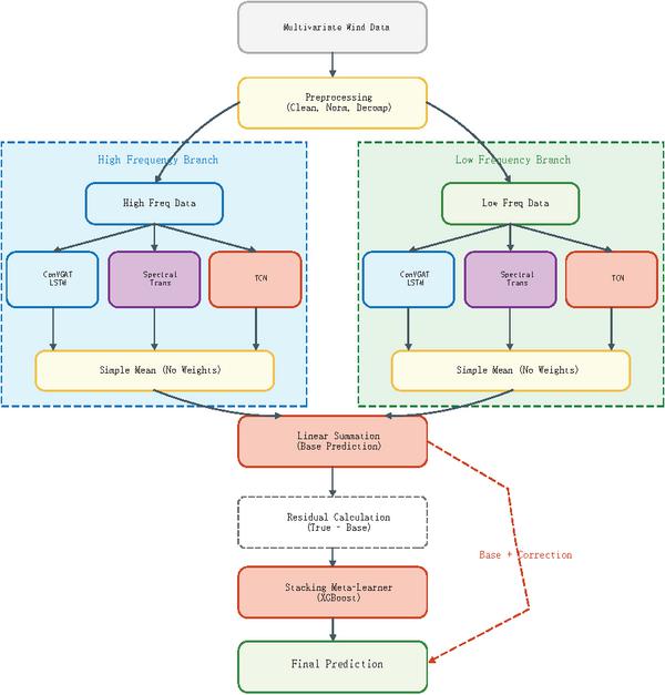
Figure 1 Overall architecture of multi-site wind energy forecasting system based on power decomposition and deep model integration.

3.3 Data Preprocessing and Power Decomposition Module

The raw data undergoes three sequential processing procedures after entering the system. Outlier detection employs the $3\sigma$ criterion-based elimination to remove observed points that meet the criterion $|x-\mu |>3\sigma$, while missing values are reconstructed through cubic spline interpolation. Normalization utilizes minimum-maximum scaling to map each feature into an interval $[0,1]$.

$${\mathrm{x}}^{\prime }=\frac{\mathrm{x}-{\mathrm{x}}_{\min }}{{\mathrm{x}}_{\max }-{\mathrm{x}}_{\min }}.$$

(13)

The power decomposition phase employs Variational Mode Decomposition (VMD), which separates the power sequence $\mathrm{p}(\mathrm{t})$ into $\mathrm{K}$ eigenmodes by solving the following constrained optimization problem:

	$\underset{{\mathrm{u}}_{\mathrm{k}},{\omega }_{\mathrm{k}}}{\min }{\displaystyle \sum _{\mathrm{k}=1}^{\mathrm{K}}}\left|{\partial }_{\mathrm{t}}\left[\left(\delta (\mathrm{t})+{\displaystyle \frac{\mathrm{j}}{\pi \mathrm{t}}}\right)\ast {\mathrm{u}}_{\mathrm{k}}(\mathrm{t})\right]{\mathrm{e}}^{-\mathrm{j}{\omega }_{\mathrm{k}}\mathrm{t}}\right|\ast 2^2,$
	$\mathrm{s}.\mathrm{t}.{\displaystyle \sum }\ast \mathrm{k}=1^{\mathrm{K}}{\mathrm{u}}_{\mathrm{k}}(\mathrm{t})=\mathrm{p}(\mathrm{t}).$	(14)

Here, ${\mathrm{u}}_{\mathrm{k}}(\mathrm{t})$ is the $\mathrm{k}$-th mode and ${\omega }_{\mathrm{k}}$ is its center frequency. The mode that satisfies ${\omega }_{\mathrm{k}}<{\omega }_{\mathrm{th}}$ is classified as the low-frequency component, while the others are classified as the high-frequency component, with the boundary defined by the intermodal frequency ${\omega }_{\mathrm{th}}=1/360$, ${\min }^{-1}$ corresponding to a 6-hour period. The low-frequency component and high-frequency component are denoted as ${\mathrm{p}}_{\mathrm{L}}(\mathrm{t})$ and ${\mathrm{p}}_{\mathrm{H}}(\mathrm{t})$, respectively, and $\mathrm{p}(\mathrm{t})={\mathrm{p}}_{\mathrm{L}}(\mathrm{t})+{\mathrm{p}}_{\mathrm{H}}(\mathrm{t})$.

3.4 Dual Branch Parallel Modeling Framework

The high-frequency and low-frequency branches are structurally identical. For each branch $\mathrm{b}\in \mathrm{H},\mathrm{L}$, let the output of the $\mathrm{m}$-th sub-model within a branch be ${\mathrm{y}}_{\mathrm{b}}^{(\mathrm{m})}$, and the branch-level prediction is achieved through simple mean merging:

$${\mathrm{y}}_{\mathrm{b}}=\frac{1}{3}\sum _{\mathrm{m}=1}^3{\mathrm{y}}_{\mathrm{b}}^{(\mathrm{m})}.$$

(15)

The theoretical basis for using a non-weighted simple mean instead of learnable weights lies in the Bias-Variance decomposition. When sub-models exhibit similar biases but low error correlations, equal-weight averaging compresses the ensemble variance to $1/\mathrm{M}$ of a single model’s variance, where $\mathrm{M}=3$, thereby avoiding overfitting risks associated with weighted parameters. The linear combination coefficients from the two branches are determined on the validation set through grid search.

$${\mathrm{y}}_{\mathrm{base}}=\alpha {\mathrm{y}}_{\mathrm{H}}+(1-\alpha ){\mathrm{y}}_{\mathrm{L}},\alpha \in [0,1].$$

(16)

3.5 ConvGAT-LSTM Submodel

Exogenous meteorological features ${\mathrm{X}}_{\mathrm{ext}}\in {ℝ}^{\mathrm{L}\times {\mathrm{F}}_{\mathrm{e}}}$ are first fed into the AFAB module, then transformed to the frequency domain via FFT, where learnable attention weights $\mathrm{A}\in {ℝ}^{\mathrm{L}/2+1}$ are applied, and finally restored through IFFT.

$${\tilde{\mathrm{X}}}_{\mathrm{ext}}=\mathrm{IFFT}(\mathrm{A}\odot \mathrm{FFT}({\mathrm{X}}_{\mathrm{ext}})).$$

(17)

The processed exogenous features are fed into a 1D CNN for local pattern extraction, and then spliced with historical power sequences ${\mathrm{X}}_{\mathrm{pow}}\in {ℝ}^{\mathrm{L}\times 1}$ to form a node feature matrix $\mathrm{H}\in {ℝ}^{\mathrm{N}\times \mathrm{d}}$. The multi-head attention network models spatial correlations between stations, with the attention coefficient between nodes defined as:

$${\alpha }_{\mathrm{ij}}^{(\mathrm{k})}=\frac{\exp (\mathrm{LeakyReLU}({\mathrm{a}}^{(\mathrm{k})\top }[{\mathrm{W}}^{(\mathrm{k})}{\mathrm{h}}_{\mathrm{i}}\parallel {\mathrm{W}}^{(\mathrm{k})}{\mathrm{h}}_{\mathrm{j}}]))}{{\sum }_{\mathrm{l}\in \mathcal{𝒩}(\mathrm{i})}\exp (\mathrm{LeakyReLU}({\mathrm{a}}^{(\mathrm{k})\top }[{\mathrm{W}}^{(\mathrm{k})}{\mathrm{h}}_{\mathrm{i}}\parallel {\mathrm{W}}^{(\mathrm{k})}{\mathrm{h}}_{\mathrm{l}}]))}.$$

(18)

The attention head index is $\mathrm{k}$, $\parallel$ represents vector concatenation, while the neighbor set $\mathcal{𝒩}(\mathrm{i})$ denotes the site’s adjacency network. GAT outputs are simultaneously fed into three parallel LSTM units, where each branch’s output undergoes temporal attention compression, and dynamic weights are computed through a variance-based weighting mechanism.

$${\mathrm{w}}_{\mathrm{m}}=\frac{\exp (-\alpha {\sigma }_{\mathrm{m}}^2)}{{\sum }_{{\mathrm{m}}^{\prime }=1}^3\exp (-\alpha {\sigma }_{{\mathrm{m}}^{\prime }}^2)},\mathrm{y}=\sum _{\mathrm{m}=1}^3{\mathrm{w}}_{\mathrm{m}}{\mathrm{y}}_{\mathrm{m}}.$$

(19)

The variance ${\sigma }_{\mathrm{m}}^2$ is the prediction variance of the $\mathrm{m}$-th LSTM on the validation window, where $\alpha$ is the temperature coefficient. The final output is $\mathrm{y}={\sum }_{\mathrm{m}=1}^3{\mathrm{w}}_{\mathrm{m}}{\mathrm{y}}_{\mathrm{m}}$.

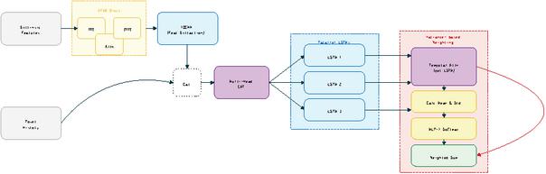
Figure 2 Convolutional graph attention transformer (ConvGAT) LSTM submodel architecture integrating AFAB frequency domain attention, multi-head graph attention network, parallel LSTM, and variance weighting mechanism.

3.6 Spectrum Transformer Submodel

Four kinds of spectral statistical features are extracted from the input sequence $\mathrm{x}\in {ℝ}^{\mathrm{L}}$ after discrete FFT transformation.

$${\mathrm{f}}_{\mathrm{spec}}=[|\mathrm{X}[\mathrm{k}]|,\mathrm{\angle }\mathrm{X}[\mathrm{k}],\mathrm{E}(|\mathrm{X}[\mathrm{k}]|),\mathrm{Std}(|\mathrm{X}[\mathrm{k}]|)]\in {ℝ}^{4\times (\mathrm{L}/2+1)}.$$

(20)

Here, $|\mathrm{X}[\mathrm{k}]|$ and $\mathrm{\angle }\mathrm{X}[\mathrm{k}]$ represent the amplitude and phase of the $\mathrm{k}$-th frequency component, respectively. These features are mapped to a ${\mathrm{d}}_{\mathrm{model}}$ dimensionality through a linear embedding layer and then fed into the Transformer encoder. The multi-head self-attention computation in the encoder is defined as:

$$\mathrm{Attention}(\mathrm{Q},\mathrm{K},\mathrm{V})=\mathrm{Softmax}\left(\frac{{\mathrm{QK}}^{\top }}{\sqrt{{\mathrm{d}}_{\mathrm{k}}}}\right)\mathrm{V}.$$

(21)

The query, key, and value matrices $\mathrm{Q}$, $\mathrm{K}$, and $\mathrm{V}$ are derived through linear projection of embedded features, with ${\mathrm{d}}_{\mathrm{k}}$ representing the key vector dimension. The encoder outputs globally averaged vectors compressed into fixed-length vectors, which are then fed into a MLP curve fitter with residual connections.

$$\mathrm{y}={\mathrm{W}}_2\cdot \mathrm{ReLU}({\mathrm{W}}_1\mathrm{z}+{\mathrm{b}}_1)+{\mathrm{b}}_2+{\mathrm{z}}_{\mathrm{res}}.$$

(22)

The pooling output $\mathrm{z}$ serves as the residual bypass signal ${\mathrm{z}}_{\mathrm{res}}$ from the encoder, effectively mitigating the gradient vanishing problem in deep MLPs.

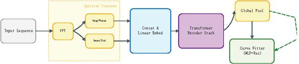
Figure 3 Structural diagram of the transformer sub-model integrating FFT spectral features with a transformer encoder stack.

3.7 Sequential Convolutional Network Submodel

The core component of TCN is the hollow causal convolution, which defines the operation on sequences $\mathrm{x}$ as:

$$(\mathrm{x}{\ast }_{\mathrm{d}}\mathrm{f})(\mathrm{t})=\sum \ast \mathrm{k}=0^{\mathrm{K}-1}\mathrm{f}(\mathrm{k})\cdot \mathrm{x}(\mathrm{t}-\mathrm{d}\cdot \mathrm{k}).$$

(23)

The hollow rate $\mathrm{d}$, representing the size of the convolution kernel $\mathrm{K}$, indicates the hollow convolution operation ${\ast }_{\mathrm{d}}$. Three cascaded convolution blocks are configured with hollow rates set sequentially as $\mathrm{d}\in 1,2,4$, corresponding to receptive fields of $\mathrm{K}$, $2\mathrm{K}-1$, and $4\mathrm{K}-3$, respectively. After three layers of stacking, the total receptive field reaches $7(\mathrm{K}-1)+1$, with the convolution kernel width $\mathrm{K}=3$ exemplifying this. The three-layer structure enables the receptive field to cover 13 time steps, effectively capturing temporal dependencies spanning from sub-hours to multi-hours. Each convolution block internally comprises:

$${\mathrm{z}}^{(\mathrm{l})}=\mathrm{Dropout}(\mathrm{ReLU}({\mathrm{Conv1D}}_{\mathrm{d}=2^{\mathrm{l}-1}}({\mathrm{z}}^{(\mathrm{l}-1)})))+{\mathrm{z}}^{(\mathrm{l}-1)}.$$

(24)

Residual connections ensure stable gradient backpropagation in deep networks, with a dropout rate of 0.2 to prevent overfitting.

Figure 4 Sub-model architecture of time-convolutional network (TCN) based on exponentially increasing void fraction.

3.8 Residual Correction Module Based on XGBoost

After the neural network components complete the basic prediction, the system enters the residual correction phase. The residual is defined as:

$${\mathrm{e}}_{\mathrm{i}}={\mathrm{y}}_{\mathrm{i}}-{\mathrm{y}}_{\mathrm{base},\mathrm{i}}.$$

(25)

The XGBoost meta-learner uses three input feature vectors: the base prediction value, independent predictions from each sub-model, and statistical summaries of original meteorological features. It iteratively learns residual mappings through gradient boosting.

$${\widehat{\mathrm{e}}}_{\mathrm{i}}^{(\mathrm{t})}={\widehat{\mathrm{e}}}_{\mathrm{i}}^{(\mathrm{t}-1)}+\eta \cdot {\mathrm{f}}_{\mathrm{t}}({\mathrm{x}}_{\mathrm{i}}).$$	(26)
$${\mathcal{ℒ}}^{(\mathrm{t})}=\sum _{\mathrm{i}=1}^{\mathrm{n}}{({\mathrm{e}}_{\mathrm{i}}-{\widehat{\mathrm{e}}}_{\mathrm{i}}^{(\mathrm{t}-1)}-{\mathrm{f}}_{\mathrm{t}}({\mathrm{x}}_{\mathrm{i}}))}^2+\gamma \mathrm{T}+\frac{\lambda }{2}{|\mathrm{w}|}_2^2.$$	(27)

Table 4 Hyperparameter settings for system modules

Module	Hyperparameter	Short-cut Process
VMD decompose	Modality K number	6
VMD decompose	Frequency threshold ${\omega }_{\mathrm{th}}$	1/360 min-1
ConvGAT-LSTM	GAT attention head count	4
ConvGAT-LSTM	Number of hidden units in parallel LSTM	64
Spectral Trans	${\mathrm{d}}_{\mathrm{model}}$	128
Spectral Trans	Number of transformer layers	3
TCN	Void fraction sequence	{1,2,4}
TCN	Convolution K kernel width	3
XGBoost	Number of trees	200
XGBoost	Learning rate $\eta$	0.05
Overall situation	History window L	48 steps (12 hours)
Overall situation	Predictive time H domain	24/48/72 steps
Data source: hyperparameter search results from the validation set, using Bayesian optimization as the search strategy and RMSE as the validation metric.

Here, $\eta =0.05$ represents the shrinkage step size, $\mathrm{T}$ denotes the number of leaf nodes in the current tree, and $\gamma$ and $\lambda$ are respectively the leaf node penalty coefficient and ${\mathrm{L}}_2$ weight regularization coefficient. XGBoost is positioned as residual learning rather than direct prediction, fundamentally leveraging gradient boosting’s strong feature-fitting capability to compensate for neural networks’ inherent limitations in capturing discontinuous transition patterns. The complementary nature of these two models in inductive bias forms the core driving logic of this design.

4 Experimental Results

4.1 Dataset Description

The experiment adopted the China National Grid Renewable Energy Generation Forecasting Competition dataset released by Chen and Xu (2022), which covers six wind farms in three types of terrain-desert, mountain, and plain-within China. The data collection spanned two years from 2019 to 2020, with a sampling interval of 15 minutes, and each site recorded approximately 35,040 valid observations annually. The recorded variables included wind speed (m/s) and wind direction ${(}^{\circ })$ at hub height, air temperature (^∘C), atmospheric pressure (hPa), and relative humidity $($ at 1.5 meters above ground, as well as the actual power output (MW) at the corresponding time. The installed capacity of the six wind farms ranged from 36 MW to 200 MW, with significant differences in the statistical dispersion of power output-Site 2 exhibited a variance of 3102.49, MW², while Site 5 was only 102.01, MW². This magnitude difference directly determined the essential differences in the challenge intensity of the prediction model’s generalization ability across sites. For missing values, cubic spline interpolation was used to handle continuous missing values of no more than four time steps, and segments exceeding the threshold were discarded, resulting in a final effective data retention rate of 98.3.

Table 5 Basic statistical characteristics of six wind farms

	Installed	Average	Power	Average
	Capacity	Power	Variance	Wind
Site	(MW)	(MW)	(MW2)	Speed (m/s)	Terrain Type
Site 1	99	23.4	580.81	6.4	Plain
Site 2	200	72.7	3102.49	7.5	Desert
Site 3	90	18.1	510.76	4.0	Mountainous region
Site 4	36	17.4	400.00	5.5	Plain
Site 5	50	6.7	102.01	4.7	Mountainous region
Site 6	150	28.8	784.00	8.1	Desert
Data source: Chen and Xu (2022), China State Grid Renewable Energy Generation Forecasting Competition Dataset.

4.2 Experimental Design and Evaluation Criteria

The dataset is divided into three time-segmented phases: 60, 20, and 20. The initial phase, approximately 18 months, is used for model training; the intermediate phase, approximately 6 months, is used for validation set hyperparameter tuning; and the final phase, approximately 6 months, serves as an independent test set. This strict temporal separation ensures that test data precedes all training and validation data, effectively eliminating forward-looking bias. For lag feature construction, power variables generate 48-order lags, covering 12-hour historical data, while meteorological variables produce 3-order lags, corresponding to $\mathrm{t}-15$, $\mathrm{t}-30$, and $\mathrm{t}-45$ min, collectively forming 67-dimensional predictive features. Three prediction timeframes are configured: 24-step (6 hours), 48-step (12 hours), and 72-step (18 hours). Each experimental group is replicated with 10 different random seeds, and results are reported as mean $\pm$ standard deviation. The experiments in this study were conducted on a computer hardware configuration with an Intel 13th Gen Intel(R) Core(TM) i9-13900HX processor and a GeForce RTX 4060 8G dedicated GPU, running on the Windows operating system, implemented in a software environment of Python 3.10 based on the PyTorch 2.6.0 framework. The evaluation metric system comprises three components:

$\mathrm{MAE}$	$={\displaystyle \frac{1}{\mathrm{N}}}{\displaystyle \sum _{\mathrm{i}=1}^{\mathrm{N}}}|{\mathrm{y}}_{\mathrm{i}}-{\widehat{\mathrm{y}}}_{\mathrm{i}}|$
$\mathrm{RMSE}$	$=\sqrt{{\displaystyle \frac{1}{\mathrm{N}}}{\displaystyle \sum _{\mathrm{i}=1}^{\mathrm{N}}}{({\mathrm{y}}_{\mathrm{i}}-{\widehat{\mathrm{y}}}_{\mathrm{i}})}^2}$
${\mathrm{R}}^2$	$=1-{\displaystyle \frac{{\sum }_{\mathrm{i}=1}^{\mathrm{N}}{({\mathrm{y}}_{\mathrm{i}}-{\widehat{\mathrm{y}}}_{\mathrm{i}})}^2}{{\sum }_{\mathrm{i}=1}^{\mathrm{N}}{({\mathrm{y}}_{\mathrm{i}}-\widehat{\mathrm{y}})}^2}}$	(28)

MAE is insensitive to outliers and reflects the overall level of prediction error; RMSE imposes a square penalty for large errors and is more sensitive to the predictive capability of climbing events; ${\mathrm{R}}^2$ quantified model explains the proportion of power variance. These three metrics complement each other and collectively form a comprehensive performance evaluation framework.

4.3 Comparison with the Baseline Model

The six baseline models span a complete spectrum from traditional single architectures to state-of-the-art approaches: CNN (Solas et al., 2019), LSTM (Li et al., 2019), CNN+Attention (Xiong et al., 2022), LSTM+CNN+Attention (Wan et al., 2023), CTRL (Hu et al., 2024b), and TCOAT (Hu et al., 2024a). Over a 24-step prediction horizon, the proposed system achieved a six-site average RMSE of $0.1065\pm 0.0021$, outperforming the closest baseline TCOAT by 1.4 and surpassing the weakest baseline LSTM+CNN by 20.8. Site 6, characterized by the highest power variance of 784.00, MW² and most complex meteorological conditions, exhibited the most dramatic performance divergence: LSTM+CNN achieved only 0.2692 at this site, highlighting the severe limitations of pure recurrent architectures under strong non-stationary conditions, while our system reached 0.7677, demonstrating an absolute improvement of 0.4985. Statistical significance was validated through site-level paired t-tests, with our system achieving significant improvements relative to all baselines $(\mathrm{p}<0.05)$. The RMSE reduction compared to LSTM+CNN+Attention reached three-star significance $(\mathrm{p}=0.0009)$, with a Cohen’s $d$ effect size of 1.68, indicating a substantial effect.

Table 6 Comparison of average performance of six stations across 24-step prediction time domains for various models in Table 6

				Relative
				Improvement
				Over LSTM
Model	Average RMSE	Average MAE	Average $R^2$	(RMSE)
LSTM	$0.1151\pm 0.0023$	$0.0760\pm 0.0015$	$0.8080\pm 0.0162$	–
CNN	$0.1208\pm 0.0024$	$0.0777\pm 0.0016$	$0.7869\pm 0.0157$	$-$4.9%
CNN+Attention	$0.1118\pm 0.0022$	$0.0728\pm 0.0015$	$0.8194\pm 0.0164$	$+$2.9%
LSTM+CNN+Attention	$0.1225\pm 0.0024$	$0.0797\pm 0.0016$	$0.7842\pm 0.0157$	$-$6.4%
CTRL	$0.1137\pm 0.0023$	$0.0747\pm 0.0015$	$0.8127\pm 0.0163$	$+$1.2%
TCOAT	$0.1080\pm 0.0022$	$0.0691\pm 0.0014$	$0.8296\pm 0.0166$	$+$6.2%
system of this paper	$0.1065\pm 0.0021$	$0.0678\pm 0.0014$	$0.8335\pm 0.0167$	$+$7.5%
Data source: Experimental results from this study, with the test set covering the post-2020 period, averaged over 10 repetitions $\pm$ standard deviation.

Table 7 Performance comparison of the proposed system with optimal baseline TCOAT across different prediction time domains

Predictive Time Domain	24 Steps (6 Hours)	48 Steps (12 h)	72 Steps (18 Hours)
This text RMSE	$0.1065\pm 0.0021$	$0.1098\pm 0.0022$	$0.1141\pm 0.0023$
TCOAT RMSE	$0.1080\pm 0.0022$	$0.1115\pm 0.0022$	$0.1163\pm 0.0023$
This text MAE	$0.0678\pm 0.0014$	$0.0699\pm 0.0014$	$0.0725\pm 0.0015$
TCOAT MAE	$0.0691\pm 0.0014$	$0.0714\pm 0.0014$	$0.0748\pm 0.0015$
This text R2	$0.8335\pm 0.0167$	$0.8262\pm 0.0165$	$0.8173\pm 0.0163$
TCOAT R2	$0.8296\pm 0.0$	$0.8221\pm 0.01$	$0.8124\pm 0.01$
Data source: Experimental results of this study, with average values calculated from six sites, repeated 10 times and averaged $\pm$ standard deviation.

As the prediction time horizon extends from 24 to 72 steps, all models show performance degradation, with our system demonstrating the lowest rate of performance decline. When measured by average RMSE, our system’s value increases from 0.1065 at 24 steps to 0.1141 at 72 steps, with a degradation rate of 7.1. In contrast, the TCOAT model shows a degradation rate of 6.9, and the LSTM+CNN model achieves a higher improvement rate of 0.1438. The widening absolute gap with extended prediction horizons highlights the enhanced advantages of frequency decomposition and multi-branch integration mechanisms in long-range prediction scenarios.

4.4 Ablation Experiment

The ablation experiments quantitatively evaluate the independent contributions of each module to overall performance by sequentially removing system components. The design logic of the seven ablation variants is as follows: Removing the VMD decomposition module (w/o Decomp) validates the effectiveness of the frequency separation strategy; Removing ConvGAT-LSTM (w/o CGL), Spectral Trans (w/o ST), and TCN (w/o TCN) respectively verifies the irreplaceability of each sub-model; Replacing variance weighting with simple mean (w/o VW) tests the value of the adaptive weight mechanism; Removing XGBoost residual correction (w/o XGB) quantifies the contribution of the post-processing layer; Degenerating multi-site joint modeling to single-site independent prediction (Single-Site) validates the necessity of cross-site spatial modeling.

Table 8 Ablation experiment results (24-step prediction time domain, average of six sites)

				Relative Increase in
				RMSE for the
Variant	Average RMSE	Average MAE	${\mathrm{R}}^2$	Complete System
Complete system	$0.1065\pm 0.0021$	$0.0678\pm 0.0014$	$0.8335\pm 0.0167$	–
w/o Decomp	$0.1189\pm 0.0024$	$0.0761\pm 0.0015$	$0.8012\pm 0.0160$	+11.6%
w/o CGL	$0.1143\pm 0.0023$	$0.0731\pm 0.0015$	$0.8124\pm 0.0162$	+7.3%
w/o ST	$0.1128\pm 0.0023$	$0.0718\pm 0.0014$	$0.8178\pm 0.0164$	+5.9%
w/o TCN	$0.1112\pm 0.0022$	$0.0708\pm 0.0014$	$0.8215\pm 0.0164$	+4.4%
w/o VW	$0.1089\pm 0.0022$	$0.0695\pm 0.0014$	$0.8281\pm 0.0166$	+2.3%
w/o XGB	$0.1098\pm 0.0022$	$0.0702\pm 0.0014$	$0.8257\pm 0.0165$	+3.1%
Single-Site	$0.1176\pm 0.0024$	$0.0752\pm 0.0015$	$0.8051\pm 0.0161$	+10.4%
Data source: Results of ablation experiments in this study, with mean $\pm$ standard deviation calculated from 10 replicates.

After removing VMD decomposition, the average RMSE increased 11.6% from 0.1065 to 0.1189, confirming the gradient conflict hypothesis of hybrid frequency signals on single models. After removing XGBoost residual correction, the RMSE rose to 0.1098, showing a small absolute increase of 3.1 that expanded to 0.1221 during 72-step long-range prediction, indicating that residual correction value increases with prediction difficulty. In single-site degradation experiments, Site 2, with power variance of 3102.49, MW², saw its RMSE deteriorate from 0.1221 to 0.1387, corresponding to a 13.6 increase, while Site 4, with power variance of 400.00, MW², only increased slightly by 2.1. Spatial modeling between sites proves significantly more beneficial for high-variability sites than low-variability ones, aligning with GAT’s mechanism design that captures meteorological coherence through dynamic attention weights.

Table 9 Comparison ${\mathrm{R}}^2$ of local RMSE between stations and climbing events

				RMSE of	LSTM RMSE	Amplitude
		This	LSTM	Climbing	for Climbing	of
Site	Topography	Text ${\mathrm{R}}^2$	${\mathrm{R}}^2$	Event	Events	Improvement
Site 1	Plain	0.7863	0.7721	0.1124	0.1456	22.8%
Site 2	Desert	0.8041	0.7875	0.1287	0.1621	20.6%
Site 3	Mountainous region	0.7935	0.7882	0.1356	0.1698	20.1%
Site 4	Plain	0.9456	0.9376	0.0812	0.1043	22.1%
Site 5	Mountainous region	0.9036	0.8679	0.1034	0.1312	21.2%
Site 6	Desert	0.7677	0.6948	0.1389	0.2134	34.9%
Data source: Experimental results from this study. The ramp-up event is defined as a period 10% during which the power fluctuation exceeds the rated capacity within 15 minutes.

4.5 Visualization and Result Analysis

The comparison of prediction curves at Site 6 reveals behavioral differences among models under extreme conditions. During the ramp-up event window, lasting approximately 45 minutes, when power output plummeted from a peak of 120 MW to below 15 MW, the standard LSTM model exhibited typical phase lag, with peak prediction delayed by about 3 time steps, equivalent to 45 minutes. In contrast, the high-frequency branch TCN sub-model in this study, leveraging a 13-step receptive field corresponding to void fraction $d=4$, preemptively captured precursor signals of power fluctuations. This reduced the local RMSE of the event from 0.2134 for the LSTM to 0.1389, achieving a significant improvement of 34.9. SHAP feature importance analysis revealed that atmospheric pressure (hPa) contributed 50.0 of total feature importance at Site 6, sharing equal importance with power history data-far exceeding other stations, where atmospheric pressure importance was consistently lower than 5. This site-specific pattern aligns closely with the physical mechanism of frequent weather fronts and pressure gradient-driven wind speed variations in the desert terrain where Site 6 is located. The findings demonstrate that the AFAB frequency-domain attention module in ConvGAT-LSTM successfully identified and amplified the most predictive meteorological signals at this site. The spatial distribution across six sites shows that the mean ${\mathrm{R}}^2$ value at mountain sites (Site 3 and Site 5) is 0.8321, lower than the 0.8660 recorded at plain sites (Site 1 and Site 4), with a difference of 0.0339. This gap indicates that complex terrain-induced local turbulence imposes a significant systematic constraint on power prediction accuracy. This explains why the relative improvement of our system at Site 3 and Site 5 compared to the baseline, with values of 5.5 and 6.8, is slightly lower than that at plain sites, Site 1 and Site 4, with values of 7.1 and 8.3.

5 Conclusion

This paper proposes a multi-site wind power forecasting system based on power decomposition and deep model integration. The system follows a four-stage paradigm of “decomposition–parallel modeling–integration–residual correction,” addressing the limitations of existing methods in mixed-frequency signal modeling, multi-site spatial correlation, and single-model generalization.

Experiments on six Chinese wind farm datasets show that the system achieves an average RMSE of $0.1065\pm 0.0021$ and ${\mathrm{R}}^2$ of $0.8335\pm 0.0167$ at the 24-step horizon, outperforming the best baseline TCOAT by 1.4 in RMSE and 0.5 in MAE $(\mathrm{p}<0.05)$. Ablation studies confirm the independent contribution of each module: VMD decomposition contributes the largest single gain ($+$11.6, multi-site joint modeling improves average RMSE by 10.4 over single-site prediction, XGBoost residual correction reduces RMSE by $3.1$ at 24 steps and 5.8 at 72 steps, and ConvGAT-LSTM reduces local ramp-event RMSE at Site 6 from 0.2134 to 0.1389 ($-$34.9. As the horizon extends to 72 steps, the system maintains the lowest performance degradation rate among all compared methods, validating the structural advantage of frequency decomposition under long-range forecasting scenarios.

Future work will focus on adaptive VMD parameter selection, probabilistic forecasting extensions, and transfer learning for newly commissioned wind farms with limited historical data.

References

[1] Chen Y, Xu J. Solar and wind power data from the Chinese state grid renewable energy generation forecasting competition[J]. Scientific Data, 2022, 9(1): 577.

[2] Hu Y, Liu H, Wu S, et al. Temporal collaborative attention for wind power forecasting[J]. Applied Energy, 2024, 357: 122502.

[3] Hu Y, Wu S, Chen Y, et al. CTRL: Collaborative temporal representation learning for wind power forecasting[C]//Proceedings of the 2024 8th International Conference on Electronic Information Technology and Computer Engineering. New York: ACM, 2024: 1219–1227.

[4] Jiang J, Han C, Wang J. Buaa_bigscity: Spatial-temporal graph neural network for wind power forecasting in Baidu KDD CUP 2022[J/OL]. arXiv preprint, 2023: arXiv:2302.11159. https://arxiv.org/abs/2302. 11159.

[5] Li J, Geng D, Zhang P, et al. Ultra-short term wind power forecasting based on LSTM neural network[C]//2019 IEEE 3rd International Electrical and Energy Conference (CIEEC). Piscataway: IEEE, 2019: 1815–1818.

[6] Sarkar M R, Anavatti S G, Ferdaus M M, et al. ASPEN-WIND: Adaptive spectral and self-supervised interactive CNN-LSTM for enhanced wind power forecasting[J]. Expert Systems With Applications, 2026, 296: 129171.

[7] Solas M, Cepeda N, Viegas J L. Convolutional neural network for short-term wind power forecasting[C]//2019 IEEE PES Innovative Smart Grid Technologies Europe (ISGT-Europe). Piscataway: IEEE, 2019: 1–5.

[8] Wan A, Chang Q, Khalil A B, et al. Short-term power load forecasting for combined heat and power using CNN-LSTM enhanced by attention mechanism[J]. Energy, 2023, 282: 128274.

[9] Wang H, Li B, Xue Z, et al. Powerformer: A temporal-based transformer model for wind power forecasting[J]. Energy Reports, 2024, 11: 736–744.

[10] Wu Q, Guan F, Lv C, et al. Ultra-short-term multi-step wind power forecasting based on CNN-LSTM[J]. IET Renewable Power Generation, 2021, 15(5): 1019–1029.

[11] Xiong B, Lou L, Meng X, et al. Short-term wind power forecasting based on attention mechanism and deep learning[J]. Electric Power Systems Research, 2022, 206: 107776.

[12] Yang M, Wang D, Xu C, et al. Power transfer characteristics in fluctuation partition algorithm for wind speed and its application to wind power forecasting[J]. Renewable Energy, 2023, 211: 582–594.

[13] Zhang Y, Kong X, Wang J, et al. Wind power forecasting system with data enhancement and algorithm improvement[J]. Renewable and Sustainable Energy Reviews, 2024, 196: 114349.

[14] Zhao S, Zhou X, Jin M, et al. Rethinking self-supervised learning for time series forecasting: A temporal perspective[J]. Knowledge-Based Systems, 2024, 305: 112652.

[15] Zheng X, Li X. Wind electricity power prediction based on CNN-LSTM network model[C]//2023 IEEE International Conference on Sensors, Electronics and Computer Engineering (ICSECE). Piscataway: IEEE, 2023: 231–236.

[16] Wang K, Tang X Y, Zhao S. Robust multi-step wind speed forecasting based on a graph-based data reconstruction deep learning method[J]. Expert Systems with Applications, 2024, 238: 121886.

[17] Dragomiretskiy K, Zosso D. Variational mode decomposition[J]. IEEE Transactions on Signal Processing, 2014, 62(3): 531–544.

[18] Huang N E, Shen Z, Long S R, et al. The empirical mode decomposition and the Hilbert spectrum for nonlinear and non-stationary time series analysis[J]. Proceedings of the Royal Society of London Series A, 1998, 454(1971): 903–995.

[19] Veličković, Cucurull G, Casanova A, et al. Graph attention networks[C]//International Conference on Learning Representations (ICLR). 2018.

[20] Chen T, Guestrin C. XGBoost: A scalable tree boosting system[C]//Proceedings of the 22nd ACM SIGKDD International Conference on Knowledge Discovery and Data Mining. New York: ACM, 2016: 785–794.

[21] Bea S, Oord A, Simonyan K, et al. WaveNet: A generative model for raw audio[J/OL]. arXiv preprint, 2016: arXiv:1609.03499. https://arxiv.org/abs/1609.03499.

[22] Vaswani A, Shazeer N, Parmar N, et al. Attention is all you need[C]// Advances in Neural Information Processing Systems (NeurIPS). 2017, 30: 5998–6008.

[23] Loshchilov I, Hutter F. Decoupled weight decay regularization[C]// International Conference on Learning Representations (ICLR). 2019.

[24] Ragab M, Eldele E, Chen Z, et al. Self-supervised autoregressive domain adaptation for time series data[J]. IEEE Transactions on Neural Networks and Learning Systems, 2022, 35(1): 1341–1351.

[25] Li Jinzhong, Xie Yuguang, Ma Wei, et al. Research on Intelligent Control Technology for Cooperative Game Implementation in Source-Grid-Load-Storage Systems Based on Reinforcement Learning[J]. Distributed Generation & Alternative Energy Journal, 2026, 41(2). DOI:10.13052/dgaej2156-3306.

[26] Wang D, Wu S. Accurate Modeling of Carbon Emissions Under Urban Energy Consumption[J]. Distributed Generation & Alternative Energy Journal, 2025, 40(05–06): 1259–1280. DOI:10.13052/dgaej2156-3306.405614.

Biographies

Zhiyi Xie (2001.05–), male, from China, is currently pursuing the M.Eng. degree in control theory and control engineering at the Faculty of Information Engineering and Automation, Kunming University of Science and Technology. His research focuses on wind power forecasting.

Zhanjun Tang (1969.07–), male, from China, received the M.S. degree in detection technology and automatic equipment from Kunming University of Science and Technology. He has worked as an assistant engineer and an engineer. He is currently a senior engineer at Kunming University of Science and Technology. His research focuses on the application of new energy sources such as wind power, solar photovoltaic power, and biomass power generation.

Wenbang Zhang (2000.10–), male, from China, is currently pursuing the M.Eng. degree in instrument and meter engineering at the Faculty of Information Engineering and Automation, Kunming University of Science and Technology. His research focuses on wind power forecasting.

Distributed Generation & Alternative Energy Journal, Vol. 41_4, 1031–1054
doi: 10.13052/dgaej2156-3306.4147
© 2026 River Publishers