A Health Condition Assessment and Safety Early Warning Framework for Hydropower Equipment Using Multi-Source Data Fusion and Decision Support Systems

Qiaofeng Lin^1,* and Shijian Wu²

¹Fujian Branch, China Huadian Corporation Limited; Minhou, Fujian, 350100, P. R. China
²Fujian Branch, China Huadian Corporation Limited; Fuzhou, Fujian, 350001, P. R. China
E-mail: linqiaofeng@chd.com.cn; shijian-wu@chd.com.cn
*Corresponding Author

Received 25 April 2026; Accepted 15 June 2026

Abstract

Hydropower plants heavily depend on the performance of turbine generators, where unexpected equipment failure can cause downtime, loss, and even safety issues in the process. The traditional condition monitoring methods mainly focus on vibration signals detected by a single sensor, which is not integrated with multiple sources and lacks the ability to perceive the risk at the plant level. In addition, the majority of the studies do not consider the equipment level health condition and structural risk factors to develop unified decision support for safety issues. To address the issues, the paper proposes a framework for the integrated health assessment and safety early warning framework, which is developed by integrating the equipment level fault diagnosis model based on the CNN-LSTM network and the structural risk assessment model developed by the GloHydroRes dataset. The novelty of the proposed multi-level data fusion framework integrates equipment-level and plant-level information for safety assessment that incorporates multi-channel vibration and torque signals along with structural attributes such as dam height, reservoir volume, and installed capacity to derive a unified safety risk index. Experimental validation using the proposed approach on the SEU multi-sensor dataset achieved high classification performance with Accuracy of 0.9634, Precision of 0.8642, Recall of 0.9613, F1-score of 0.9065, and MCC of 0.8662. Moreover, multi-class ROC analysis indicated high performance with AUC values of 0.9936 (Low Risk), 0.9930 (Medium Risk), and 0.9997 (High Risk), outperforming individual CNN, LSTM, and Random Forest approaches. The unified safety index revealed that 46.6% of samples were classified as Low Risk, 34.1% of samples were classified as Medium Risk, and 19.3% of samples were classified as High Risk, thus validating the efficacy of the proposed decision support mechanism. Compared with traditional fault detection methods, the proposed approach improves the reliability of fault prediction results, reduces false alarm rates, and enables proactive maintenance decisions based on risk considerations.

Keywords: Multi-source data fusion, CNN–LSTM, hydropower equipment monitoring, structural risk index, safety early warning system.

1 Introduction

Hydropower energy is one of the most important aspects in the development of renewable and low-carbon energy systems in the world [1]. Modern hydropower equipment includes sophisticated turbine generator sets, gear sets, bearings, and other equipment that can operate under high mechanical and hydraulic loads [2]. Continuous operation under dynamic loads, cavitation, and other environmental factors can cause equipment degradation [3]. Conventional equipment monitoring in hydropower equipment is mainly based on single-point measurements or threshold-level SCADA alarms, which cannot detect potential issues in equipment operation [4]. With the aging of equipment in hydropower plants, it is more and more important to ensure equipment operation reliability and equipment structure safety [5]. With the development of new sensor technologies and industrial IoT, it is possible to acquire multi-channel signals of vibration, torque, and operating status, and the fusion of diverse information sources in safety intelligence is a research hotspot [6].

In terms of application, it is found that intelligent systems of health condition evaluation are highly useful in making predictive maintenance plans for hydropower stations highly effective [7]. This is because complex systems of machine learning algorithms are able to evaluate potential issues before a complete failure occurs [8]. This is highly useful because potential issues are identified at earlier stages, and economic losses are reduced by planning maintenance in advance. In addition to equipment variables such as vibration and torque sensors, variables such as plant variables like dam height and capacity are also included in the systems for enhanced risk awareness [9]. DSS are also highly useful in making predictive evaluations for maintenance planning and risk stratification. These systems are highly useful for the safe and efficient running of hydropower stations in the context of increased variability in climate and load [10]. An algorithm for detecting ECG abnormalities to support automated cardiac condition analysis and improve diagnostic accuracy [11]. An integrated and scalable architecture for cost-effective remote health monitoring through efficient healthcare data management and communication [12].

To solve the aforementioned problems, this paper proposes a hierarchical system for assessing the health conditions and safety early warning system based on multi-source data fusion and the CNN-LSTM predictive model. The proposed system will perform sensor-level fusion for equipment classification, considering the plant-level structural risk factors for safety assessment. The system will also develop a probabilistic safety early warning system for predicting the degree of faults and the corresponding staged warnings. Moreover, the system will develop a decision support system for calculating the overall safety index for decision-making. Compared with the traditional single-layer monitoring system, the proposed system will integrate equipment health diagnosis and structural risk analysis from a holistic perspective. The effectiveness of the proposed CNN-LSTM predictive model for improving the accuracy of equipment faults will be verified by the experimental results.

Research Questions

• Does multi-channel fusion improve fault classification accuracy?

• Can CNN-LSTM capture fault progression effectively?

• Does structural risk modeling improve final safety prediction?

• Can DSS reduce operational safety risks?

The rest of the paper is structured as follows: in Section 2, the related work is presented, including the existing research on hydropower equipment monitoring, multi-source data fusion, deep learning-based fault diagnosis, and decision support systems. In Section 3, the problem statement is presented, including the research objectives and challenges. In Section 4, the methodology used in this research is presented. Specifically, the data preprocessing, multi-source fusion strategy, CNN-LSTM model, structural risk modeling, and decision support are presented. In Section 5, the experimental design is presented, including the dataset design, model training processes, and evaluation metrics. In Section 6, the experimental results are presented, including performance analysis, comparison, and discussions. Finally, in Section 7, the conclusions are presented, including potential future research directions.

2 Related Works

Zhang et al. [13] proposed a multi-source information fusion model for the early warning of the production environment safety of coal mines [14]. The multi-source heterogeneous sensors used were temperature sensors, dust sensors, wind speed sensors, vibration energy sensors, and gas sensors. The early warning system used the proposed model and developed an early warning index system based on factor analysis and principal component analysis [15]. The multi-input single-output and multi-input multi-output models were developed at the feature level based on the BP neural network. The accuracy of the proposed system reached 89.29%, which proves the feasibility of the system for scientific decision-making for the safety management of the coal mines. An innovative structural health monitoring system for a hydro-steel structure was proposed by Li et al. [16] based on the finite element method, multi-sensor data fusion, and IoT technology for the closed-loop system [17]. The proposed system was used for the spillway of the Luhun Reservoir. The monitoring results showed that dynamic values of stress increased by 2 MPa during the radial gate operation and were still within the permissible limits. There were also no significant impact loads [18]. The results also showed that the vibration amplitude was maintained below 0.03 mm, which ensured safety. Shao et al. [19] developed a framework for safety and sustainable management of reservoirs using an integrated information system approach. The framework incorporated different aspects such as multiple sensors’ data fusion and correlation mechanisms for heterogeneous data and a cross-coupled analytical model [20]. The framework was implemented at the Ye Fan Reservoir in Hubei Province of China. The framework integrated different modules such as flood dispatching, safety monitoring, warning systems, and video monitoring to establish a three-dimensional perception network [21]. The application of the framework improved the accuracy and reliability of the system and ensured scientific decision-making. This proved the effectiveness of the framework in modern reservoir management [22].

Li et al. [23] proposed a digital twin framework for hydraulic engineering, aiming at improving monitoring, risk prediction, and optimizing hydraulic systems. They proposed a five-dimensional digital twin framework based on multi-source data fusion, GIS and BIM integration, and real-time virtual and physical interaction [24]. The proposed framework was implemented for the Danjiangkou Project, and the results showed improved accuracy for deformation monitoring, water quality simulation, and geological hazard prediction. Additionally, improved operation efficiency, safety management, and prediction performance were observed for hydraulic management when compared to traditional hydraulic management methods. Zhao et al. [25] proposed a conceptual framework for sustainable management of water reserves based on digital twin technology, IoT-based water monitoring, game engine simulation, and AI-based DSS [26]. The conceptual framework was able to create a digital twin environment through the integration of IoT sensors, GIS maps, remote sensing, UAV-based digital elevation models, and machine learning models. The results of the simulation showed the accuracy of the prediction of flooding based on varying rainfall intensity, early warning systems of drought based on soil moisture and flow rates, and real-time water quality notifications. Liu et al. [27] conducted a systematic literature review (SLR) and bibliometric-qualitative analysis (BQA) on the use of DT technology in the field of water conservancy and hydropower engineering at the watershed scale [28]. The research showed significant research gaps in terms of information integration, BIM process alignment with construction processes, and information governance. Based on the research gaps, a new Watershed Information Modeling (WIM) approach was proposed, which integrated BIM+ models with knowledge-driven decision-making. This research was able to provide a solution to the application of smart watershed management [29].

Zhang et al. [30] proposed a group of comprehensive standards for intelligent operation and maintenance (O&M) to address the limitations of manual operation, disorderly management of data, and digital integration of intelligent buildings and municipal facilities [31]. According to the theory of operation management, these standards were divided into three dimensions: functional services (perception, data fusion, decision-making, and disaster prevention), system hierarchy (perception, human-computer interaction), and intelligence characteristics (monitoring, autonomous maintenance) [32]. Besides, the paper also examined the present standards and applications to help readers validate the proposed framework. The proposed framework provides a reference for developing standard intelligent operation and maintenance systems theoretically and practically. Liu et al. [33] carried out a systematic review of the latest developments in integrating AI with tunnel boring machines (TBM), especially regarding environmental perception, autonomous control, and health prediction. They proposed the system architecture for intelligent TBM with the help of DT technology, which includes the perception, analysis, decision, and execution layers to achieve autonomous control over the entire process [34]. The proposed architecture has the ability to solve issues such as complex geology, rock-machine interaction, and coordination problems. The authors have also identified the key issues associated with the process, such as data integration, interpretation, and efficiency. Zhao et al. [35] proposed an intelligent curing control system for face slab concrete with the help of multi-source measurement data and real-time monitoring with the IoT. The system included cloud data analysis, feedback control, and a decoupled front-end and back-end visualization system for temperature monitoring and intelligent control [36]. The system was applied in the Maerdang concrete face rockfill dam (CFRD) project in a high-altitude cold region, achieving temperature exceedance prediction and dynamic curing adjustment. The application of the system proved its effectiveness in real-time monitoring and curing control [37].

Despite their important achievements, there are some limitations that can be found in these studies. Zhang et al. [13] reached 89.29% accuracy for the prediction of coal mine safety; however, their BP neural network model might encounter scalability and generalization issues in more dynamic coal mine environments. Li et al. [16] proved the effectiveness of the SHM system in a single hydro-steel structure, but generalization to other types of hydraulic structures was not considered. The same is applicable to Shao et al. [19], who demonstrated the effectiveness of their system in the management of the Ye Fan Reservoir but did not extensively explore the large-scale validation in other areas. The proposed Digital Twin models by Li et al. [23] and Zhao et al. [25] demonstrated the better monitoring and prediction capabilities, but the issues with real-time data synchronization, high computational complexity, and integration complexity remain unsolved. Liu et al. [27] identified the challenges associated with the implementation of DT in the watershed scale, but their study is conceptual with fewer large-scale real-world applications. The intelligent O&M standards proposed by Zhang et al. [30] provide a systematic approach to intelligent systems. However, standardization and industrialization still pose as challenges. In another study by Liu et al. [33], the challenges associated with interpretability, efficiency, and data integration in intelligent TBM systems have been identified. Such studies indicate that there are still technical barriers to be cleared to attain complete autonomy in intelligent systems. Although the intelligent curing system proposed by Zhao et al. [35] in a dam construction project has been successful, its applicability in different conditions needs to be empirically verified.

3 Problem Statement

Although there have been major breakthroughs and developments in the area of intelligent monitoring, digital twin, and AI-based infrastructure management systems, there are still some major issues that have not been addressed adequately by the current models and systems, as highlighted by Li et al. [23]. The current models have been tested under specific conditions and scenarios, which makes them less scalable and more specific to certain geographical locations and conditions, as highlighted by Li et al. [16]. Additionally, the current data architecture also makes it difficult to achieve the required integration and interoperability with different data sources such as IoT sensors, BIM, GIS, and remote sensing systems, as highlighted by Liu et al. [33]. The high computational complexity and synchronization delay also make it difficult to achieve the required decision-making capabilities, and the lack of interpretability makes it less useful for management personnel.

Objectives

• Develop a hierarchical health condition assessment and safety early warning framework for hydropower equipment that integrates multi-source data fusion with a risk-aware decision support system to enhance operational reliability, predictive maintenance, and plant-level safety management.

• Utilize the SEU multi-channel rotating machinery dataset for equipment-level health modeling and the GloHydroRes global hydropower dataset for plant-level structural and reservoir risk modeling, enabling multi-layer contextual safety assessment.

• Design and implement a CNN–LSTM-based multi-source data fusion model that extracts spatial and temporal features from vibration and torque signals for accurate fault classification and early warning prediction.

• Construct a structural risk index using hydropower plant attributes and integrate it with equipment fault probability to generate a unified safety risk score supporting maintenance prioritization and operational decision-making.

4 Methodology

Based on the above analysis, this paper proposes a health condition assessment and safety early warning system for hydropower equipment based on multi-source data fusion and a CNN-LSTM decision support model. First, different types of data sources, such as vibration signals, temperature data, operating conditions, and environmental conditions, are collected and synchronized with respect to time through time alignment and missing value preprocessing. Then, noise removal and normalization operations are completed, and time and frequency domain feature extraction operations are accomplished. The CNN model is used for automatic extraction of spatial and local degradation features, and the LSTM model is used for extraction of the equipment degradation trends. The fused features are used for classification and safety early warning. The model is evaluated from the following aspects: accuracy, precision, recall, and F1 score. The proposed model is used as a decision support system for the online health monitoring and predictive maintenance of hydropower equipment.

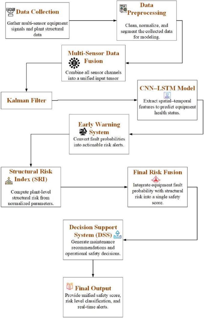
Figure 1 Integrated multi-source data fusion and CNN–LSTM-based safety early warning framework for hydropower equipment.

The data is preprocessed and multi-sensor fusion is carried out to obtain a unified input for the model. The CNN-LSTM model is used to extract spatial-temporal features to obtain the equipment health state and fault probability. The structure parameters are separately processed to obtain the SRI. The fault probability predicted from the equipment-level model and the structural risk information are integrated within the fusion module to compute the final safety score, as shown in Figure 1. A Kalman Filter is applied at the sensor level to fuse real-time measurements and improve the accuracy of equipment health estimation.

4.1 Multi-Source Data Fusion

In this research, data fusion means that different kinds of data are integrated to obtain a more accurate and reliable safety prediction result for hydropower equipment. Rather than relying on a single vibration signal, the system uses several signals and structural information to obtain a comprehensive safety assessment.

4.1.1 Sensor-level data fusion (equipment level)

At the equipment level, eight different monitoring signals are combined. These include:

• Motor vibration

• Gearbox vibrations (X, Y, and Z directions)

• Torque measurements

These signals are combined in the following manner:

• Time-aligned

• Noise-filtered

• Normalized

• Combined into a single input dataset

This technique is known as early fusion. Here, all the signals from the sensors are combined before sending them into the CNN-LSTM model.

4.1.2 Deep learning feature fusion

Inside the CNN-LSTM model, we have the following components:

• The CNN model extracts spatial fault patterns from the vibration signal.

• The LSTM model learns the development of faults over time.

The feature fusion is internally carried out, and a reliable fault probability and health classification are generated.

This helps the system to detect:

• Sudden faults

• Gradual degradation

4.1.3 Risk-level fusion (plant level integration)

Besides the equipment signals, the system also includes the following types of structural information:

• Dam height

• Reservoir volume

• Installed capacity

• Type of plant

These inputs are used to derive a Structural Risk Index (SRI).

Finally, the system combines:

• Fault probability of the equipment (dynamic risk)

• Structural Risk Index (static risk)

This yields a Final Safety Risk Score.

Plant type is incorporated into the Structural Risk Index (SRI) because different hydropower configurations are exposed to varying operational and structural risk conditions. Storage hydropower plants generally exhibit higher risk due to the presence of large reservoirs, higher hydraulic loads, and potentially severe consequences associated with dam-related failures. Pumped-storage facilities experience additional operational stress resulting from frequent load variations and cyclic pumping–generation operations, which may accelerate mechanical wear and structural fatigue. In contrast, run-of-river plants typically operate with smaller storage capacities and lower hydraulic pressures, resulting in comparatively lower structural risk. Therefore, plant-type weighting is included to reflect differences in operational stress patterns, structural behavior, and potential failure impacts, thereby improving the realism of plant-level safety assessment.

4.2 CNN–LSTM Model Design

The CNN-LSTM architecture is intended to capture both the spatial and temporal features of the signals from the hydropower equipment. The convolutional layers are used to extract local vibration features related to mechanical faults. The LSTM layers are used to capture the evolution of degradation with time. The output layer is used to classify the health state and estimate the risk. The CNN–LSTM architecture was selected because it effectively combines spatial feature extraction and temporal sequence modeling within a unified framework. The CNN component automatically identifies local fault-related patterns from multi-sensor vibration signals, whereas the LSTM component captures long-term temporal dependencies associated with equipment degradation and fault evolution. Compared with standalone CNN or LSTM models, the hybrid CNN–LSTM approach provides a more comprehensive representation of both spatial and temporal characteristics, making it particularly suitable for hydropower equipment health assessment and early warning applications. This combination offers a favorable balance between predictive accuracy, computational efficiency, and model interpretability.

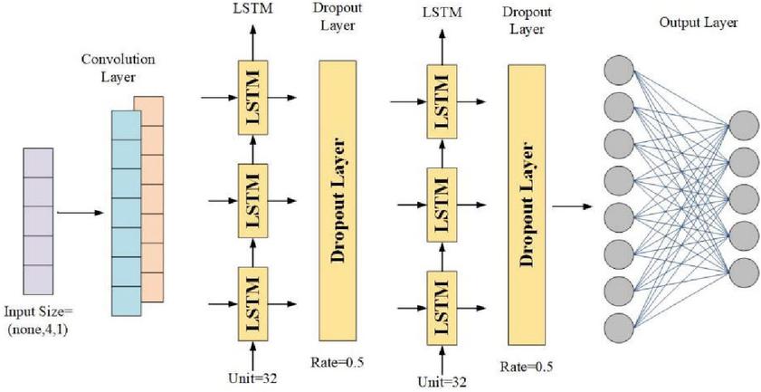
Figure 2 CNN–LSTM hybrid architecture with dropout regularization.

The model receives a sequential input of shape (None, 4, 1). It starts processing this input through a Convolutional layer for local feature extraction. The features extracted are then passed through stacked LSTM layers of 32 units each for sequential feature learning. A Dropout layer of rate 0.5 is added for overfitting avoidance. The process of sequential feature learning continues through another set of LSTM layers and Dropout. The final prediction is made through a fully connected Output layer as shown in Figure 2.

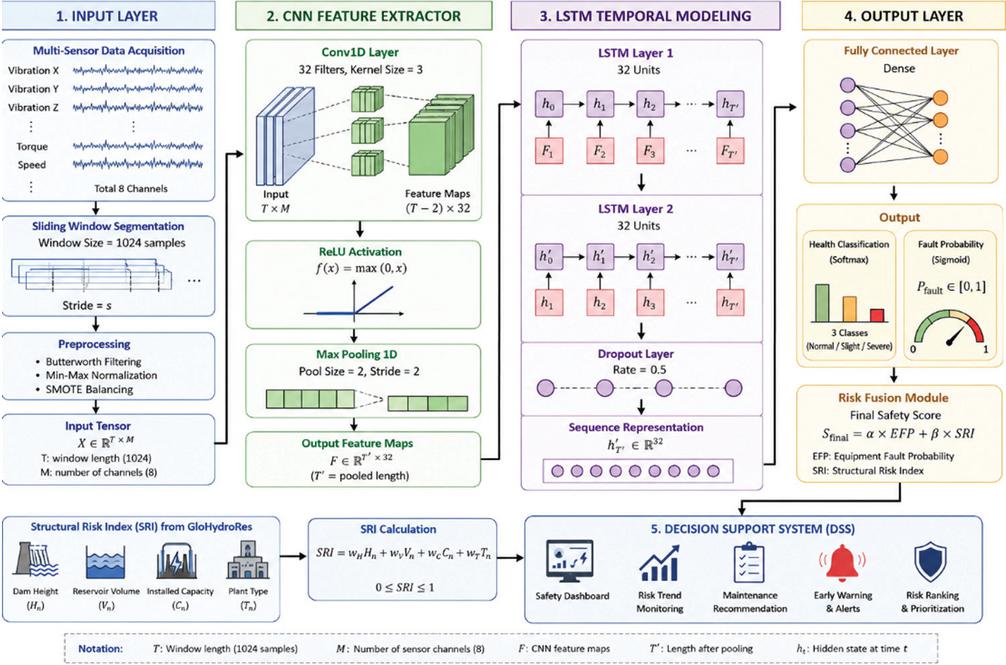
Figure 3 CNN–LSTM-based multi-source framework for hydropower safety assessment and early warning.

Figure 3 illustrates the overall architecture of the proposed multi-source health condition assessment and safety early warning framework. The framework begins with the acquisition of multi-sensor vibration and torque signals, which are segmented using a sliding-window approach and subsequently preprocessed through noise filtering, normalization, and class balancing techniques. The processed data are then supplied to a one-dimensional CNN module that extracts spatial fault-related features from the sensor signals. These feature maps are forwarded to stacked LSTM layers to capture temporal dependencies and degradation patterns associated with equipment faults. Table 1 shows the CNN–LSTM model architecture for extracting features and classifying input data into three classes.

Table 1 CNN–LSTM architecture specifications

Layer Type	Output Shape	Parameters	Activation
Input Layer	1024 $\times$ 8	0	–
Conv1D (32 filters, k $=$ 3)	1022 $\times$ 32	Trainable	ReLU
MaxPooling1D (pool $=$ 2)	511 $\times$ 32	0	–
LSTM (32 units)	32	Trainable	tanh
LSTM (32 units)	32	Trainable	tanh
Dropout (0.5)	32	0	–
Dense (Softmax)	3 classes	Trainable	Softmax

The proposed CNN–LSTM architecture processes multi-channel sensor data through a Conv1D layer and max-pooling operation to extract and reduce spatial features efficiently. The resulting feature maps are then analyzed by two stacked LSTM layers to capture temporal dependencies and fault progression patterns in the signal sequence. Finally, a dropout layer mitigates overfitting, while a dense Softmax layer performs multi-class fault classification by generating the probability of each equipment health condition.

4.2.1 CNN component – spatial feature extraction

The CNN module is responsible for processing multi-channel vibration data obtained from the hydropower system. The CNN module extracts spatial features related to faults, such as peaks and amplitude modulation. The convolutional kernels are used to scan the time series data to learn the spatial features. Pooling is applied to reduce the dimensionality of the features and remove noise. Dropout is used to improve generalization.

Input Representation: This Equation (1) defines the multi-channel vibration input signal. $T$ represents total time steps in the signal window. $C$ represents the number of sensor channels. Each element $x_{t,c}$ is the signal value at time $t$ and channel $c$. This structured representation enables multi-sensor feature learning.

$$X=\{x_{t,c}\},t=1,\mathrm{\dots },T,c=1,\mathrm{\dots },C$$

(1)

1D Convolution Operation: This Equation (2) computes convolution for the $k$-th filter. The kernel slides over time window $K$. Weights $W_{k,c,i}$ study spatial correlations across channels. Bias term $b_k$ adjusts activation offset. This process extracts localized fault signatures from vibration signals.

$$Z_k(t)=\sum _{c=1}^C\sum _{i=0}^{K-1}{W}_{k,c,i}\cdot x_{t+i,c}+b_k$$

(2)

ReLU Activation: ReLU makes the model non-linear. Negative values are set to zero. Positive values remain as they are. This improves the non-linear discriminative ability of the model. It prevents vanishing gradient issues as shown in Equation (3).

$$A_k(t)=\max (0,Z_k(t))$$

(3)

Max Pooling: Max pooling selects the highest activation within region $\mathrm{\Omega }$. It reduces the temporal dimension of the feature maps. Dominant vibration peaks are retained, and noise and minor fluctuations are suppressed. This improves computational efficiency as shown in Equation (4).

$$P_k(t)=\underset{j\in \mathrm{\Omega }}{\max }{A}_k(t+j)$$

(4)

Dropout: Dropout randomly deactivates neurons during training. $\mathit{r}$ is a binary mask sampled from Bernoulli distribution. Probability $p$ controls neuron retention rate. This prevents co-adaptation of features. It improves generalization on unseen data as shown in Equation (5).

$${\tilde{P}}_k(t)=P_k(t)\cdot r$$

(5)

Algorithm 1: CNN-Based Spatial Feature Extraction
Input: Multi-channel vibration signals
Output: Extracted spatial fault features
Step 1: Prepare Input
Collect vibration signals from multiple sensors.
Arrange them into fixed time windows.
Step 2: Apply Convolution
Slide filters over the signal.
Detect important fault patterns like peaks and amplitude changes.
Step 3: Apply ReLU Activation
Remove negative values.
Keep important positive features.
Step 4: Apply Max Pooling
Keep the strongest features.
Reduce noise and data size.
Step 5: Apply Dropout
Randomly disable some neurons during training.
Prevent overfitting and improve generalization.
Step 6: Output Features
Send the extracted spatial features to the LSTM layer for further processing.

4.2.2 LSTM component – temporal dependency modeling

The LSTM layer represents the degradation process over time in hydropower systems. The LSTM layer extracts the long-term temporal dependencies in the vibration signals. Conventional RNNs have problems with gradient vanishing. The LSTM layer uses gating to regulate the flow of information.

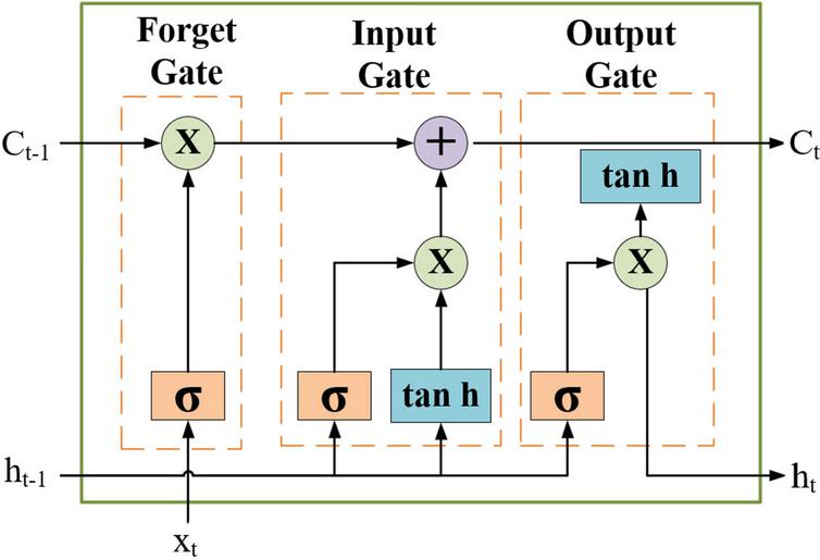
Figure 4 Architecture of LSTM.

This Figure 4 describes the internal structure of the Long Short-Term Memory (LSTM), which is utilized for modeling the temporal dependencies. The forget gate manages the information that needs to be forgotten from the previous memory cell. The input gate manages the information that needs to be stored from the current input. Finally, the output gate manages the information that needs to be passed to the next hidden state for further processing. This structure of the LSTM avoids instability while training the model, making it appropriate for fault progression analysis.

Forget Gate: The forget gate determines which past information to discard. It uses sigmoid activation to output values between 0 and 1. Values close to 0 indicate forgetting. Values close to 1 indicate retaining memory. This prevents irrelevant historical influence as shown in Equation (6).

$$f_t=\sigma (W_f[h_{t-1},x_t]+b_f)$$

(6)

Input Gate: The input gate controls how much new information enters memory. It combines previous hidden state and current input. Sigmoid activation functions control the intensity of updating. Higher values permit new information to be added. Lower values restrict memory updates as indicated in Equation (7).

$$i_t=\sigma (W_i[h_{t-1},x_t]+b_i)$$

(7)

Candidate Cell State: This Equation (8) produces candidate memory content. Tanh activation maps values between $-$1 and 1. It represents potential new degradation information. This candidate state is filtered by the input gate. Ensures controlled memory updates.

$${\overline{C}}_t=\tanh (W_c[h_{t-1},x_t]+b_c)$$

(8)

Cell State Update: The cell state stores long-term temporal memory. Previous state is multiplied by forget gate. New candidate information is weighted by input gate. Element-wise multiplication ensures selective updating. This maintains stable degradation trend tracking as shown in Equation (9).

$$C_t=f_t\circ C_{t-1}+i_t\circ {\tilde{C}}_t$$

(9)

Output Gate: The output gate controls visible hidden state. Sigmoid function scales output between 0 and 1. It regulates how much memory influences output. Ensures stable temporal representation. Prevents sudden activation spikes as shown in Equation (10).

$$o_t=\sigma (W_o[h_{t-1},x_t]+b_o)$$

(10)

Hidden State: Hidden state represents final LSTM output at time $t$. Cell state is activated using tanh. Output gate filters relevant information. This produces time-aware feature representation. It is passed to classification layer as shown in Equation (11).

$$h_t=o_t\odot \tanh (C_t)$$

(11)

Algorithm 2: LSTM for Temporal Dependency Modeling in Hydropower Equipment
Input: Sequential vibration and torque sensor data
Output: Time-aware feature representation for fault classification
Steps:
Step 1: Initialize LSTM Memory
Start with empty memory to store historical information about equipment health.
Step 2: Forget Gate Operation
Decide which past information is no longer relevant and can be discarded.
Helps prevent irrelevant historical data from affecting current predictions.
Step 3: Input Gate Operation
Determine how much new information from current sensor data should be added to memory.
Balances between old knowledge and new observations.
Step 4: Candidate Memory Generation
Create a potential new memory update based on the current input.
Represents possible degradation or fault patterns emerging over time.
Step 5: Update Cell State
Combine the retained old memory and the new candidate information.
Ensures the memory reflects both long-term trends and recent changes.
Step 6: Output Gate Operation
Decide which information from the cell state should influence the output at the current time
step.
Controls what the model “reveals” for the classification layer.
Step 7: Compute Hidden State
Generate the final time-aware feature representation for the current step.
Pass this hidden state to the classification or fault probability layer.
Step 8: Repeat for Each Time Step
Process all sequential measurements to capture the complete degradation pattern over time.
Step 9: Pass to Classification Layer
Use the extracted temporal features to classify equipment health (Normal/Slight/Severe)
or compute fault probability.

4.2.3 Output layer – health classification & risk scoring

The output layer undertakes two prediction processes. It is responsible for the classification of health states into three groups. It is also involved in the estimation of continuous fault probability. The softmax activation function deals with multi-class classification. The sigmoid function is involved in probabilistic early warning scoring.

Softmax: Softmax converts logits into probabilities. Total probability sums to one. Each class receives normalized likelihood. Highest probability determines predicted class. Suitable for multi-class health classification as shown in Equation (12).

$$P(y=k|x)=\frac{e^{z_k}}{{\sum }_{j=1}^3{e}^{z_j}}$$

(12)

Sigmoid: Sigmoid produces a value between 0 and 1. Represents continuous fault likelihood. Higher values indicate higher risk. Thresholds can trigger early warning. Supports decision support systems as shown in Equation (13).

$$P_{\mathrm{fault}}=\frac{1}{1+e^{-z}}$$

(13)

Final Risk Fusion: This Equation (14) integrates operational and structural risks. $P_{\mathrm{fault}}$ comes from CNN-LSTM prediction. ${\mathrm{Risk}}_{\mathrm{structural}}$ comes from reservoir dataset. Weights $\alpha$ and $\beta$ balance contributions. It produces unified safety risk index.

$${\mathrm{Risk}}_{\mathrm{final}}=\alpha P_{\mathrm{fault}}+\beta {\mathrm{Risk}}_{\mathrm{structural}}$$

(14)

4.3 Early Warning Mechanism

4.3.1 Risk stage conversion

The CNN-LSTM model provides a continuous probability of faults at each time step. But the risk levels required by the operators are in categories, not probabilities. Hence, a probability-to-risk level mapping mechanism is incorporated. This helps in better interpretability of results in real-time hydropower systems.

Fault Probability Output: The variable $z_t$ represents the raw output (logit) of the CNN-LSTM model. The sigmoidal function transforms this value into a bounded probability. The exponential term ensures smooth nonlinear chance scaling. The output $P_f(t)$ lies strictly between 0 and 1. This probabilistic form allows threshold-based risk classification as shown in Equation (15).

$$P_f(t)=\sigma (z_t)=\frac{1}{1+e^{-z_t}}$$

(15)

Risk Stage Classification: The function is a piecewise classification form. The lower bound of 0.3 represents minor anomaly behavior. The region between 0.6 and 0.3 represents high and elevated but non-failure conditions. The upper bound of 0.6 represents high fault likelihoods. This is a discretized form of continuous risk and is shown in Equation (16).

$$R(t)=\{\begin{array}{cc}\mathrm{Normal},\hfill & 0\le P_f(t)<0.3\hfill \\ \mathrm{Warning},\hfill & 0.3\le P_f(t)<0.6\hfill \\ \mathrm{Critical},\hfill & P_f(t)\ge 0.6\hfill \end{array}$$

(16)

4.3.2 Early warning alert generation

Individual probability peaks may lead to false alarms in real-life systems. Therefore, there is a need to smooth the time series to guarantee the validation of persistence before activating the alarm system. The moving average system will guarantee the validation of persistence before the alarm is activated. This will lead to robustness in the hydropower system.

Temporal Smoothing: The Equation (17) computes the normal probability over a window of size $N$. It aggregates recent historical predictions for stability. Short-term fluctuations are summary through smoothing. The parameter $N$ controls sensitivity to recent behavior. This filtered likelihood is used for reliable alert decisions.

$${\overline{P}}_f(t)=\frac{1}{N}\sum _{i=0}^{N-1}{P}_f(t-i)$$

(17)

Alert Activation Function: The binary variable $A(t)$ represents alert status. Threshold $\theta$ defines activation sensitivity. If smoothed probability exceeds threshold, alert is triggered. Otherwise, system remains in monitoring state. Different thresholds produce warning and critical alerts as shown in Equation (18).

$$A(t)=\{\begin{array}{cc}1,\hfill & {\overline{P}}_f(t)\ge \theta \hfill \\ 0,\hfill & {\overline{P}}_f(t)<\theta \hfill \end{array}$$

(18)

4.3.3 Lead time estimation

Lead time is a measure of how early a problem is forecasted to occur. It provides a forecast of the usefulness of the early warning system. The higher the lead time, the better it is for proactive maintenance planning. This will ensure that economic and operational losses are minimized. Lead time is therefore a key factor in evaluation.

Lead Time Definition: Where: ${\mathit{t}}_{\mathit{f}}=$ actual fault time, ${\mathit{t}}_a=$ first alert activation time. The Equation (19) is used for calculating the time difference between fault and alert. The positive sign of this equation represents successful early detection, zero sign represents that fault and detection occur simultaneously, and negative sign represents delayed prediction. This equation directly measures the system’s responsiveness.

$$T_{\mathrm{lead}}=t_f-t_a$$

(19)

Average Lead Time: The formula modes lead times over multiple fault events. The flexible $M$ This is the total number of failures, which provides the overall performance of the early warning system. The effects of the outliers are reduced using the averaging method, which facilitates the statistical reliability evaluation using Equation (20).

$${\overline{T}}_{\mathrm{lead}}=\frac{1}{M}\sum _{j=1}^M(t_{f,j}-t_{a,j})$$

(20)

4.3.4 Escalation timeline modeling

Risk Growth Rate: The derived measures are used to measure the instantaneous change in risk. The slope is positive in case of increasing failure probabilities. The greater the slope, the greater is the rate of degradation. The slope is nearly zero in case of a stable condition. This measure is used in escalation detection, as described in Equation (21).

$$\frac{d{P}_f(t)}{dt}$$

(21)

Critical Time Projection: The equation linearly extrapolates risk to critical threshold. The numerator represents remaining risk margin. The denominator represents growth rate of probability. The ratio estimates time to reach critical state. This enables proactive scheduling before system failure as shown in Equation (22).

$$t_c=t+\frac{0.6-P_f(t)}{\frac{d{P}_f(t)}{dt}}$$

(22)

4.4 Structural Risk Modeling (Plant-Level)

This assesses the natural vulnerability of the infrastructure of hydropower plants based on static physical parameters. Contrary to health monitoring, which relies on sensors, this phase considers design-related risk parameters that are not time variant. The aim is to express the natural structural risk prior to incorporating operational information. Based on the attributes of the GloHydroRes dataset, risk parameters are standardized and aggregated. The result is a Structural Risk Index (SRI) ranging from 0 to 1 for each plant.

4.4.1 Dam height risk modeling

The height of the dam is an important engineering feature that symbolizes the potential energy of the hydraulic system stored in the dam. The higher the dam, the higher the hydrostatic pressure on the structural walls. The structural stress is directly proportional to the height of the water column. The effect of failure is more severe in the case of a higher dam due to the force of gravity.

Dam Height Normalization: This Equation (23) applies Min-Max normalization to dam height. It rescales all height values into a 0–1 interval. $H_i$ represents the height of the ith plant. $H_{\min }$ and $H_{\max }$ represent dataset bounds. Higher normalized values indicate relatively taller and potentially higher-risk dams.

$$H_{\mathrm{norm}}=\frac{H_i-H_{\min }}{H_{\max }-H_{\min }}$$

(23)

4.4.2 Reservoir volume risk modeling

Reservoir volume is the total amount of water mass behind the dam. Large volumes create considerable horizontal stress on the retaining walls. Reservoirs with high volumes pose a considerable flood risk to the downstream area during failure. Fluctuations in the seasons can accentuate the stress cycles. Hence, the reservoir volume is a direct factor in the exposure to structural hazards.

$$V_{\mathrm{norm}}=\frac{V_i-V_{\min }}{V_{\max }-V_{\min }}$$

(24)

This formula standardizes reservoir volume across all plants. It ensures comparability regardless of measurement scale. $V_i$ is the reservoir volume of plant i. Minimum and maximum values defining dataset range. Higher normalized scores indicate larger stored hydraulic mass as shown in Equation (24).

4.4.3 Installed capacity risk modeling

Installed capacity represents the scale of energy production of a plant. Large-capacity plants have higher cycles of mechanical loads. Large plants are important points in the power grid of a country. The economic effect of a failure in a large plant is higher. Thus, installed capacity represents the risk of operational criticality.

Installed Capacity Normalization: This Equation (25) normalizes installed capacity into a 0-1 scale. It eliminates unit-based magnitude differences. $C_i$ represents plant generation capacity. Dataset bounds prevent extreme bias from large values. Higher normalized values correspond to higher systemic importance.

$$C_{\mathrm{norm}}=\frac{C_i-C_{\min }}{C_{\max }-C_{\min }}$$

(25)

4.4.4 Plant type risk weight modeling

Hydropower plants are differentiated structurally according to design. Run-of-river plants exert low storage pressure. Storage dams have large reservoirs with high structural stress. Pumped storage plants have cyclic operations with pressure variations. Therefore, the plant types are transformed into numerical risk weights.

Plant Type Weight Assignment: This piecewise function maps qualitative categories to quantitative weights. Weights reflect engineering risk severity levels. Run-of-river plants are assigned lowest structural risk weight. Pumped-storage systems receive higher weight due to cyclic stress. The assigned weight directly contributes to final risk aggregation as shown in Equation (26).

$$T_w=\{\begin{array}{cc}0.3\hfill & \text{Run-of-River}\hfill \\ 0.6\hfill & \text{Storage}\hfill \\ 0.8\hfill & \text{Pumped Storage}\hfill \end{array}$$

(26)

4.4.5 Structural risk index (SRI) aggregation

The Structural Risk Index integrates all the normalized factors. This is a measure of overall infrastructure risk. The factors are weighted proportionally. This is done based on their relative engineering value. The final score of SRI is between 0 and 1.

Structural Risk Index: This Equation (27) performs weighted linear combination. Each regularized factor is multiplied by its assigned weight. The constraint ensures total inspiration equals unity. ${\mathit{SRI}}_1$ represents structural risk of plant i. Output is bounded between 0 (lowest risk) and 1 (highest risk).

$${\mathit{SRI}}_i=w_1{H}_{\mathrm{norm}}+w_2{V}_{\mathrm{norm}}+w_3{C}_{\mathrm{norm}}+w_4{T}_w$$

(27)

4.4.6 Structural risk classification

After determining SRI, plants are grouped based on risk levels. This facilitates prioritization of maintenance activities. There are thresholds that group plants based on safety levels during operations. This makes it easier to understand. This facilitates integration with early warning systems.

Risk Level Classification This piecewise function categorizes the risk levels. The threshold of 0.33 identifies low vulnerability plants. The threshold of 0.66 identifies high structural exposure. The values in between represent moderate risk. These values can be used to determine the inspection schedule for safety, as indicated in Equation (28).

$$\mathrm{Risk}\mathrm{Level}=\{\begin{array}{cc}\mathrm{Low}\hfill & \mathrm{SRI}<0.33\hfill \\ \mathrm{Medium}\hfill & 0.33\le \mathrm{SRI}<0.66\hfill \\ \mathrm{High}\hfill & \mathrm{SRI}\ge 0.66\hfill \end{array}$$

(28)

4.5 Integrated Safety Risk Score

4.5.1 Equipment fault probability

The probability of equipment failure represents the probability of abnormal operation of hydropower equipment. The probability of equipment failure can be obtained with the CNN-LSTM predictive model based on deep learning. The probability reflects the dynamic equipment degradation behavior. The probability reflects the equipment operation uncertainty in real-time. The probability of equipment failure is the dynamic equipment risk in the integrated equipment safety framework.

Fault Probability Output: The hidden state $h_t$ represents learned temporal features from sequential sensor inputs. The linear change $W_o{h}_t+b_o$ maps extracted features into a risk-related scalar value. The weight matrix $W_o$ controls the contribution of each latent feature. The sigmoid initiation function $\sigma (\cdot )$ compresses the output into a probability range between 0 and 1. Thus, $P_f$ directly represents the forecast probability of equipment failure as shown in Equation (29).

$$P_f=\sigma (W_o{h}_t+b_o)$$

(29)

4.5.2 Structural risk index

The structural risk index is a measure of risk with respect to plant-level characteristics of hydropower infrastructure. This includes information related to dam geometry, reservoir size, and capacity. This is related to the severity of consequence risk. This is not dynamic equipment risk, which is considered static over a very short-term horizon. The Structural Risk Index (SRI) is a normalized composite indicator that quantifies the overall structural and operational risk level of a hydropower plant based on key characteristics such as dam height, reservoir volume, installed capacity, and plant type. Higher SRI values indicate greater potential safety risks and operational vulnerability.

Structural Risk Aggregation: Each normalized structural parameter ${\widehat{x}}_i$ characterizes a scaled infrastructure feature. The weight coefficient $w_i$ reflects the relative safety importance of that feature. The summation aggregates all weighted attributes into a unified structural risk value. Higher weights are assigned to critical parameters such as dam height or reservoir volume. The final result $S_r$ quantifies overall structural weakness as shown in Equation (30).

$$S_r=\sum _{i=1}^n{w}_i\cdot {\widehat{x}}_i$$

(30)

Min-Max Normalization: The raw structural variable $x_i$ may have different units and magnitudes. Min-max regularization rescales values into the $[0,1]$ interval. The term $x_{\min }$ and $x_{\max }$ define the observed feature bounds. This prevents dominance of large-scale variables in weighted summation. Normalized structures ensure fair contribution in structural risk computation as shown in Equation (31).

$${\widehat{x}}_i=\frac{x_i-x_{\min }}{x_{\max }-x_{\min }}$$

(31)

4.5.3 Integrated safety risk score

The integrated safety risk score is a combination of the probability of equipment failure and the structure risk. This provides the basis to integrate multi-source data within a single platform for decision-making. The model provides weighted importance to the dynamic and static risk factors. This is a combination of the likelihood of failure and the severity of the consequences.

Final Integrated Risk: The coefficient $\alpha$ represents the weight of equipment failure prospect. The coefficient $\beta$ represents the weight of structural vulnerability. The linear grouping provides an interpretable risk aggregation method. Both inputs are normalized, ensuring the final score remains within $[0,1]$. The resulting $R_{\mathrm{final}}$ reflects overall hydropower operational safety level as shown in Equation (32).

$$R_{\mathrm{final}}=\alpha P_f+\beta S_r$$

(32)

Weight Constraint: This avoids artificial inflation of risk magnitude. Typical settings use $\alpha =0.6$ and $\beta =0.4$. Weights can be optimized using validation experiments or expert judgment as shown in Equation (33).

$$\alpha +\beta =1$$

(33)

4.6 Multi-Source Data Fusion (Sensor Level)

In this research, multi-source data fusion is conducted at the sensor level based on early fusion, where all the available sensor data are fused prior to feature extraction and model training. In particular, eight different monitoring signals, including vibration in multiple directions, temperature, pressure, rotational speed, and acoustic signals, are synchronized, normalized, and aligned with a common time axis. Subsequently, all the signals are stacked together to construct a comprehensive three-dimensional input tensor with the format (Samples $\times$ Time Steps $\times$ 8 Channels). In this case, each sample corresponds to one observation window, which is derived through sliding time segmentation, the time steps indicate the sequential measurements within the observation window, and the eight channels indicate the different sensors. Through this early fusion method, the CNN layers are capable of automatically learning the cross-sensor spatial correlations, and the LSTM layers are able to capture the temporal dependencies in the time domain.

Kalman Filter for Sensor Data Fusion

In this paper, the signals of equipment states, such as vibration, torque, temperature, and pressure, which are obtained through multi-sensors, are used to monitor the health condition of the equipment in the hydropower station. However, there may exist some noise and errors in the signals of each single sensor, which may influence the accuracy of equipment fault detection. Therefore, in this paper, the Kalman Filter method is used to improve the accuracy of sensor signals.

With the Kalman Filter method, the accurate states of equipment can be estimated in real time according to the signals of each sensor. The accurate states of equipment obtained through the Kalman Filter method can better reflect the health condition of equipment.

With the accurate states of equipment obtained through the Kalman Filter method, the input tensor of the CNN-LSTM model can be formed, and the equipment fault probability can be obtained through the CNN-LSTM model. Finally, the Final Safety Risk Score can be obtained according to the equipment fault probability and the structural states of the equipment in the hydropower station.

4.7 Decision Support System (DSS)

The DSS combines the results of multi-source data fusion into operational intelligence. The Decision Support System translates raw fault predictions and structural risk results into management decisions. The DSS is hierarchical in nature, from equipment to plant and portfolio. The Decision Support System is useful for predictive maintenance and safety control decisions. The Decision Support System facilitates proactive hydropower safety management.

Safety Dashboard

The Safety Dashboard is a comprehensive graphical representation of the health status of the hydropower plant. It combines dynamic equipment fault probability with static structural risk factors. The Safety Dashboard is updated continuously with real-time data from the monitoring system. It uses standardized safety indices to display risk levels. This module improves operator awareness and decision-making capabilities.

$$R_t=\alpha P_f(t)+\beta S_r$$

(34)

The term $P_f(t)$ represents the time-dependent equipment fault probability obtained from the CNN-LSTM model. The term $S_r$ denotes the structural risk index derived from plant attributes and reservoir characteristics. The weighting factors $\alpha$ and $\beta$ determine the relative importance of dynamic and static risks. The constraint $\alpha +\beta =1$ ensures normalized risk contribution. The resulting $R_t$ quantifies the overall real-time safety condition of the plant as shown in Equation (34).

Maintenance Recommendation Engine

The Maintenance Recommendation Engine identifies the best time for intervention. It considers both the magnitude of risk and the rate of growth of risk. The system gives priority to assets that are deteriorating at a faster rate. It reduces unnecessary expenses on maintenance.

$$M_u=\frac{d{P}_f(t)}{dt}+\gamma R_t$$

(35)

The derivative term $\frac{d{P}_f(t)}{dt}$ measures the rate of fault probability increase over time. A larger derivative indicates accelerated degradation. The term $R_{\mathrm{t}}$ incorporates the overall system risk context. The coefficient $\gamma$ adjusts sensitivity to cumulative risk. The maintenance urgency index $M_u$ determines scheduling priority as shown in Equation (35).

Risk Ranking of Plants

The Risk Ranking module is used to assess and compare several hydropower plants. The module gives a systematic approach to prioritize the allocation of inspections. Both equipment and structural levels are taken into account. The module is applicable on a regional or national level for safety management. The module improves the efficiency of strategic asset management.

$${\mathit{RR}}_4=w_1{\overline{P}}_{f,i}+w_2{S}_{r,i}$$

(36)

The term ${\overline{P}}_{f,i}$ represents the average equipment fault probability of plant $i$. The structural index $S_{r,i}$ captures inherent infrastructure vulnerability. Weights $w_1$ and $w_2$ balance operational and structural risks. The constraint $w_1+w_2=1$ maintains normalization. Plants are ranked based on descending values of ${\mathit{RR}}_{\mathrm{i}}$ as shown in Equation (36).

Operational Adjustment Advisory

The Operational Adjustment Advisory module suggests dynamic load control strategies. The purpose is to minimize mechanical stress during high-risk situations. Load reduction prevents rapid component deterioration. The advisory module adjusts itself to real-time safety status. This ensures safe and sustainable power production.

$$L_{\mathrm{adj}}=L_{\max }(1-R_t)$$

(37)

The term $L_{\max }$ represents the maximum permissible operating load. The safety score $R_t$ determines the proportion of risk exposure. When risk increases, the factor ($1-R_t$) decreases. This proportionally reduces operational load. The model ensures adaptive stress mitigation during high-risk periods as shown in Equation (37).

Emergency Inspection Alert System

The Emergency Inspection Alert System is a very important safety notification system. It identifies critical situations that require immediate attention. The system operates at pre-defined safety thresholds. The system acts as a preventive measure for major failures. This module improves the readiness of the emergency response system.

$$E_a=\{\begin{array}{cc}1,\hfill & R_t\ge {\theta }_c\hfill \\ 0,\hfill & R_t<{\theta }_c\hfill \end{array}$$

(38)

The threshold ${\theta }_c$ signifies the critical safety boundary. If $R_t$ exceeds this threshold, an alert is triggered. The binary output simplifies operational decisions. Threshold correction is performed using validation datasets. This mechanism balances false alarms and missed findings as shown in Equation (38).

Early fusion refers to the integration of heterogeneous feature representations at the input or feature-extraction stage. In this study, deep features extracted from the CNN–LSTM-based fault diagnosis model are concatenated with structural risk indicators obtained from the SRI model prior to classification. This strategy enables the learning algorithm to capture cross-domain interactions between equipment-level degradation patterns and plant-level structural conditions, resulting in a more informative and discriminative joint feature space for improved risk prediction.

5 Experimental Setup

5.1 Data Collection

SEU Dataset

The main dataset used for this research is Southeast University (SEU) Drivetrain Dynamics Simulator Dataset [38]. This dataset was collected from a laboratory-scale rotating machinery test rig designed and built at Southeast University, China. For this research, the dataset was collected using synchronous multi-channel vibration and torque signals of a simulated drivetrain environment under various working and faulty conditions. In other words, there are eight synchronous sensor signals in the dataset, and these signals contain motor vibration, planetary gearbox vibration in three orthogonal directions (X, Y, Z), parallel gearbox vibration in three orthogonal directions (X, Y, Z), and motor torque measurements under two different working conditions based on different speed-load combinations.

The different types of faults included in the dataset, such as bearing and gear faults, are important for supervised classification of the health condition of the system. The synchronized and multi-directional nature of the signals are more representative of multi-sensor industrial monitoring, which is typical in the turbine generator assembly in the hydropower plant. For this study, the SEU dataset will be used as the primary equipment-level dataset to evaluate the proposed CNN-LSTM-based health condition assessment model. The dataset is appropriate for multi-sensor data fusion, fault classification, and predictive warning modeling. The dataset is appropriate to evaluate the deep learning model, which will be able to exploit the characteristics of the signal (spatial features using convolutional layers) and the degradation process (using LSTM layers). Although the system is laboratory-scale, the dynamic characteristics of the rotating machinery are representative of the hydropower turbine generator system.

GloHydroRes

The secondary data used in this research comes from GloHydroRes (Global Hydropower and Reservoir Dataset) [39], which can be accessed freely via Zenodo. GloHydroRes integrates open-source hydropower plant data with reservoir data to form a huge hydropower reservoir with 7,775 hydropower plants in 128 countries. The GloHydroRes dataset comprises 29 variables that describe the structural, operational, and hydrological characteristics of hydropower plants. The most important variables for this research are installed capacity, dam height, reservoir depth, reservoir surface area, reservoir volume, plant type (such as run-of-river, storage, and pumped storage), and related river data.

Contrary to the SEU dataset, GloHydroRes does not include equipment-level vibration or sensor time-series data. Rather, it includes plant-level context attributes that shape overall operational risk and safety exposure. In this study, GloHydroRes is employed to build a Structural Risk Index, which symbolizes the macro-level safety and operational risk of hydropower plants. Variables like dam height and reservoir volume are normalized and used in the proposed decision support system (DSS) as context risk attributes. The Decision Support System (DSS) is designed to transform the predicted Equipment Fault Probability (EFP) and Structural Risk Index (SRI) into an interpretable overall safety index for operational decision-making. The DSS integrates outputs from both the CNN–LSTM-based fault diagnosis model and the structural risk evaluation module to compute a unified safety score. The proposed framework combines plant-level structural attributes with equipment-level failure probabilities to create a hierarchical safety evaluation system that improves risk awareness beyond the scope of isolated sensor-based monitoring.

The addition of GloHydroRes enhances the proposed framework by allowing multi-level data fusion, where micro-level equipment health forecasts are integrated with macro-level infrastructure risk indicators. This is beneficial for a more comprehensive safety early warning system and enhances the effectiveness of decision-making in the management of hydropower systems.

The multi-channel vibration and torque signals provide complementary information about the mechanical condition of rotating components under different operating states. Vibration signals capture fault-related dynamic behavior, while torque measurements reflect load variations and transmission characteristics. The integration of these synchronized sensor signals enables the CNN-LSTM model to learn discriminative fault patterns more effectively, thereby improving classification accuracy and early fault detection capability.

5.2 Data Preprocessing

The preprocessing stage ensures data consistency through time synchronization and missing value handling. Time synchronization aligns multi-sensor signals to a common temporal reference to ensure uniform sampling across all channels. Missing values are addressed using interpolation techniques to maintain continuity in the dataset and prevent information loss during model training. These steps are performed once in a unified preprocessing pipeline to avoid redundancy and improve computational efficiency.

IoT-based sensing systems to enable continuous monitoring of hydropower equipment and infrastructure. Distributed sensors collect real-time vibration, torque, and operational measurements, which are transmitted through connected monitoring networks for centralized analysis. This IoT-enabled architecture supports real-time data fusion by integrating information from multiple sensing sources, thereby improving data availability, situational awareness, and fault detection reliability.

5.2.1 SEU dataset preprocessing

Signal Segmentation

The sliding window segmentation technique helps to transform the continuous vibration signal into structured samples. This technique helps to enable the deep learning model to process fixed-length inputs. This technique helps to preserve the local temporal information in each segment. It also helps to increase the number of effective training samples. It helps to improve the sensitivity of fault detection in the early stages.

Raw Signal Representation: The function $x(t)$ represents the vibration signal over time. $t$ denotes discrete sampling instances. $T$ is the total signal length. This signal is collected from vibration sensors. It forms the original input for preprocessing as shown in Equation (39).

$$x(t),t=1,2,3,\mathrm{\dots },T$$

(39)

Windowed Segment: ${\mathit{X}}_{\mathit{i}}$ represents the ith segmented window. $L$ is the window length. Each segment contains consecutive signal samples. The segment captures localized temporal behavior. It becomes one training instance for CNN-LSTM as shown in Equation (40).

$$X_i=\{x(i),x(i+1),\mathrm{\dots },x(i+L-1)\}$$

(40)

Number of Segments: $S$ is the stride length between windows. $T-L$ ensures full window coverage. The floor function ensures integer segment count. Larger stride reduces sample number. This determines total training dataset size as shown in Equation (41).

$$N=\lfloor \frac{T-L}{S}\rfloor +1$$

(41)

Noise Filtering

Noise filtering eliminates high-frequency noise. Mechanical signals are often contaminated with environmental noise. Butterworth filter has smooth frequency response. It does not have ripple distortion in the passband. It is used to improve the signal quality before feature extraction.

Butterworth Transfer Function: $H(j\omega )$ defines filter frequency response. $\omega$ represents signal frequency. ${\omega }_c$ is cutoff frequency. $n$ is filter order controlling slope sharpness. Higher frequencies beyond cutoff are attenuated as shown in Equation (42).

$$H(j\omega )=\frac{1}{\sqrt{1+{(\frac{\omega }{{\omega }_c})}^{2n}}}$$

(42)

Filtered Signal: $y(t)$ is filtered output signal. The transfer function modifies frequency components. Noise components are suppressed. Important mechanical frequencies are preserved. The output is cleaner for modeling as shown in Equation (43).

$$y(t)=H(j\omega )\cdot x(t)$$

(43)

Normalization (Min-Max Scaling)

Normalization rescales feature values. Sensor values have varying magnitudes. Unscaled features can bias neural networks. Min-Max scaling restricts data to a fixed range. It speeds up gradient-based optimization.

Min-Max Scaling: $x_{min}$ is minimum observed value. $x_{\max }$ is maximum observed value. The numerator shifts data to zero baseline. The denominator scales values proportionately. Output lies between 0 and 1 as shown in Equation (44).

$$x_{norm}=\frac{x-x_{\min }}{x_{\max }-x_{\min }}$$

(44)

Dataset Balancing

Imbalance Ratio: $N_{\mathrm{majority}}$ is dominant class sample count. $N_{\mathrm{minority}}$ is rare class sample count. Developed ratio indicates severe imbalance. Balanced datasets method ratio of 1. This metric guides sampling decisions as shown in Equation (45).

$R={\displaystyle \frac{N_{\mathrm{majority}}}{N_{\mathrm{minority}}}}$

(45)

SMOTE Sample Generation: $x_i$ is minority sample. $x_{nn}$ is nearest neighbor. $\lambda$ is random value between 0 and 1. New sample is direct interpolation. This increases minority representation as shown in Equation (46).

$$x_{\mathrm{new}}=x_i+\lambda (x_{nn}-x_i)$$

(46)

The Synthetic Minority Oversampling Technique (SMOTE) was applied during the preprocessing stage. SMOTE generates synthetic samples for underrepresented fault categories by interpolating between existing minority-class observations. This balancing process prevents the learning model from becoming biased toward majority classes and promotes more uniform representation of all fault conditions during training.

Kalman Filter-Based Signal Estimation

The Kalman Filter is a recursive state estimation algorithm that combines noisy sensor observations with prior state predictions to generate an optimal estimate of the true system state. By continuously correcting measurement errors and reducing random noise, the filter enhances signal stability and consistency across multiple sensor channels. In the proposed framework, the Kalman Filter is applied to vibration and torque signals before feature extraction. This process improves the reliability of sensor data, minimizes fluctuations caused by measurement uncertainty, and provides more stable inputs for the CNN–LSTM model. Consequently, the fusion of multiple sensor streams becomes more robust, leading to improved fault diagnosis and safety assessment performance.

5.2.2 GloHydroRes dataset preprocessing

Missing Value Handling

Mean Imputation: $N$ characterizes number of available samples. Summation adds all known values. Mean value is believed from existing data. Missing entries are replaced by this mean. This preserves dataset completeness as shown in Equation (47).

$$x_{\mathrm{miss}}=\frac{1}{N}\sum _{i=1}^N{x}_i$$

(47)

Feature Normalization (Standardization)

The characteristics of the hydropower structure have different scales. The scale of the dam height and capacity is not equal. Standardization eliminates scale bias. Standardization ensures equality in the comparison of values. Standardization improves the stability of the structural index calculation.

Z-Score Normalization: $\mu$ is feature mean. $\sigma$ is standard deviation. Deducting mean centers the data. Dividing by standard deviation normalizes spread. Result has zero mean and unit modification as shown in Equation (48).

$$x_{\mathrm{scaled}}=\frac{x-\mu }{\sigma }$$

(48)

Structural Risk Factor Computation

Structural risk is a function of physical parameters. Dam height is a factor in hydrostatic pressure. Reservoir volume is a factor in load stress. Installed capacity is a factor in operational criticality. These factors are used to calculate composite risk index.

Structural Risk Index: $H,V,C$ are normalized features. $w_i$ are importance weights. Weights reflect engineering priorities. Sum of weights ensures bounded output. Higher SRI indicates higher structural risk as shown in Equation (49).

$$\mathit{SRI}=w_{1}H+w_{2}V+w_{3}C$$

(49)

Weight Constraint: This ensures total contribution equals 100%. It maintains regularized risk range. Prevents over-amplification of one factor. Supports multi-criteria decision modeling. Ensures mathematical consistency as shown in Equation (50).

$$w_1+w_2+w_3=1$$

(50)

Installed Capacity Risk Integration

It affects overall safety criticality. Capacity is a factor in final risk fusion. It connects equipment level and plant level risk.

Capacity Normalization: $C_{\min }$ is minimum capacity value. $C_{\max }$ is maximum capacity value. The formula rescales capacity values. Output lies between 0 and 1. Ensures uniform contribution to risk index as shown in Equation (51).

$$C_{\mathrm{norm}}=\frac{C-C_{\min }}{C_{\max }-C_{\min }}$$

(51)

Final Integrated Risk: $P_{\mathrm{fault}}$ is CNN-LSTM predicted probability. $SRI$ is structural risk index. $\alpha$ and $\beta$ are fusion weights. Their sum equals 1. Final score supports safety early warning as shown in Equation (52).

$$R_{\mathrm{final}}=\alpha P_{\mathrm{fault}}+\beta SRI$$

(52)

Data Splitting

Once the GloHydroRes dataset is preprocessed (missing values handled, normalization done on the features, and structural risk factors computed), the next step is the division of the dataset into training, validation, and testing sets.

• Training Set: This is the set where the model is created and where the associations between the plant-level variables (features) such as the dam height, volume, capacity, and plant type with the structural risk index are learned.

• Validation Set: This is the set where the parameters of the model are adjusted and the optimal weights for the aggregation of the risk values are learned, avoiding overfitting.

• Testing Set: This is the set where the performance of the structural risk modeling and the final safety risk score with the equipment fault probability is evaluated.

Algorithm 3: Data Preprocessing
Input: Vibration data (SEU) + Structural data (GloHydroRes)
Output: Final integrated risk score
Step 1: Segment raw vibration signal using sliding window.
Step 2: Filter noise using Butterworth filter.
Step 3: Normalize signal values (0–1 scaling).
Step 4: Balance dataset using SMOTE if classes are imbalanced.
Step 5: Handle missing values using mean imputation.
Step 6: Standardize structural features.
Step 7: Compute Structural Risk Index using weighted features.
Step 8: Normalize installed capacity.
Step 9: Combine CNN–LSTM fault probability with Structural Risk Index.
Step 10: Generate final safety risk score and trigger warning if needed.

5.3 Hardware Configuration

The system uses an Intel Core i7-14700 CPU, which has a base processor frequency of 2.10 GHz. This is a part of Intel’s 14th generation family of CPU products, which includes several performance and efficiency cores that enable parallel execution of compute-intensive tasks.

The system also uses a DDR4 RAM type with a capacity of 32.0 GB and a memory type speed of 3200 MT/s, which makes it efficient for handling multitasking operations. This is a high-capacity RAM type that makes it efficient for handling large batch data processing, feature extraction, and simultaneous execution of data loading and model training processes, which is extremely beneficial when executing data fusion processes for experimentation.

For the graphical and accelerated computing needs of the system, the computer is equipped with an NVIDIA GeForce GT 730 GPU with 4 GB dedicated video RAM. Though the computer is not equipped with a high-performance GPU suitable for deep learning tasks, the GPU still supports the execution of matrix-based and neural network-based computing tasks through its support for CUDA. The GPU is mainly useful in the execution of the convolutional layers in the CNN layers and is useful in the faster convergence of the model during the experiment.

The computer is based on a 64-bit x64 architecture, which is suitable for the execution of modern machine learning frameworks such as TensorFlow and PyTorch. The computer is also running on a 64-bit version of the Windows 11 Home operating system with Version 25H2. The computer is also equipped with a total of 466 GB of storage capacity, out of which approximately 266 GB is available for use.

The computer is adequately equipped with the required computing resources to ensure the implementation of the proposed framework for health assessment and safety early warning through the proposed CNN-LSTM architecture.

5.4 Software Configuration

The experimental implementation of the proposed multi-source health assessment and safety early warning framework has been carried out using a well-structured and integrated software environment. The proposed framework has been developed using PyCharm 2025.3.11 as an integrated development environment (IDE) for debugging, coding, and project organization. The programming language used for the proposed framework is Python 3.9, which is one of the most stable and widely used programming languages.

For developing deep learning models, PyTorch has been used as a prominent framework because it has the ability to support a dynamic computation graph. The proposed CNN-LSTM model has been developed using PyTorch modules. The proposed model has customized convolutional, pooling, and recurrent neural network layers. The baseline models, such as individual CNN, LSTM, and Random Forest classifiers, have been developed using Scikit-learn. The parameters for evaluating the model, i.e., Accuracy, Precision, Recall, F1-score, and ROC-AUC Score, have been computed using the Scikit-learn library. Although the proposed framework primarily deals with the health assessment of the machinery, the proposed framework has utilized the Hugging Face Transformers library for text-based metadata processing or incorporating it with the maintenance logs.

For the pre-processing of the data as well as signal processing, Pandas, NumPy, and SciPy libraries have been utilized. This has helped in efficiently processing multiple channel data received from the vibration sensor. Signal fusion from multiple sources was performed using NumPy operations to fuse the sensor data from the eight-channel sensor system. This resulted in unified tensor data that was appropriate for inputting the data into the CNN architecture. SQLite/HDF5 was used for the storage of structured data as well as for efficient retrieval of the stored data. In addition, Matplotlib/Seaborn libraries were used for visualization as well as performance analysis. Furthermore, Plotly/Dash libraries were used in developing an interactive decision support system that can be used for visualizing the risk levels. Finally, the computation of the Structural Risk Index and Safety Score was done using Pandas as well as NumPy libraries. In conclusion, the Decision Support System (DSS) interface was created using a Graphical User Interface (GUI), which enabled efficient monitoring as well as decision support for hydropower equipment safety management.

5.5 Hyperparameter Configuration of CNN–LSTM Model

CNN Component

• Number of convolutional layers: 1–2

• Number of filters: 32 filters per layer

• Kernel size: 3

• Activation function: ReLU

• Pooling: Max Pooling, pool size = 2

• Dropout: 0.5

LSTM Component

• Number of LSTM layers: 2 stacked layers

• Number of units per LSTM layer: 32 units

• Dropout between layers: 0.5

• Activation: tanh (for hidden state)

• Recurrent activation: sigmoid

Output Layer

• Health classification: Softmax activation (3 classes: Normal / Slight / Severe)

• Fault probability: Sigmoid activation (range 0–1)

Training Parameters

• Optimizer: Adam

• Learning rate: 0.001

• Batch size: 32

• Epochs: 100

• Loss function: Categorical Cross-Entropy (classification) + Binary Cross-Entropy (fault probability)

5.6 Evaluation Metrics

Accuracy

Accuracy measures the correctness of the classification model in general terms. It calculates the number of correct classifications out of all the predictions made. It considers normal as well as fault classifications. It is applicable when the dataset is balanced. However, it may not be the best performance metric to use with an unbalanced fault dataset.

$$\mathrm{Accuracy}=\frac{\mathrm{TP}+\mathrm{TN}}{\mathrm{TP}+\mathrm{TN}+\mathrm{FP}+\mathrm{FN}}$$

(53)

The term TP $+$ TN represents all correctly classified samples. The denominator TP $+$ TN $+$ FP $+$ FN represents total predictions made by the model. The equation is a measure of calculating the ratio of correct predictions and total predictions made by the model. The equation is a global measure of classification effectiveness. The result of the equation varies between 0 and 1, and its highest value is 1 as shown in Equation (53).

Precision

Precision is the reliability of the prediction of faults. It is the number of predicted faults, which are actually faults. It focuses on reducing the number of false alarms in the system. High precision means less maintenance. It evaluates the quality of positive predictions.

$$\mathrm{Precision}=\frac{\mathrm{TP}}{\mathrm{TP}+\mathrm{FP}}$$

(54)

Here TP stands for the number of correct instances of faults. The denominator TP $+$ FP stands for all instances of faults. The equation above computes the ratio of correct instances of faults. If false positives go up, then precision drops significantly. The value will be between 0 and 1. Higher values indicate fewer false alarms as shown in Equation (54).

Recall (Sensitivity)

Recall is the ability of the model to identify real faults. It measures the number of real faults that are correctly predicted by the model. It mainly focuses on minimizing the number of faults that are not predicted by the model. In safety systems, recall is very important to avoid failures.

$$\mathrm{Recall}=\frac{\mathrm{TP}}{\mathrm{TP}+\mathrm{FN}}$$

(55)

The denominator TP $+$ FN represents all actual fault instances. The equation calculates the proportion of real faults detected. If false negatives increase, recall decreases significantly. The value ranges from 0 to 1, where 1 indicates no missed faults as shown in Equation (55).

F1-Score

F1-score combines precision and recall into a single measure. It is particularly helpful in imbalanced classification tasks. It discourages large discrepancies between precision and recall. It gives a harmonic mean and not an arithmetic mean. It ensures that there is a balanced assessment of the fault detection capability.

$$\mathrm{F1}=2\times \frac{\mathrm{Precision}\times \mathrm{Recall}}{\mathrm{Precision}+\mathrm{Recall}}$$

(56)

The numerator multiplies precision and recall and scales by 2. The denominator is the sum of precision and recall. The harmonic mean ensures both metrics contribute equally. If either precision or recall is low, F1-score decreases sharply. The value ranges between 0 and 1, where 1 represents optimal balanced performance as shown in Equation (56).

6 Result and Discussion

In this section, experimental verification of the proposed multi-level health condition assessment and safety early warning method is performed. First, the effectiveness of the proposed CNN-LSTM model is verified by using the SEU multi-sensor data set to evaluate its accuracy of fault classification, learning ability of temporal degradation, and effectiveness of early warning. Comparative experiments with other models (CNN, LSTM, and RF) are performed to verify the superiority of the proposed model. Then, structural health indicators of plant-level risks are calculated by using GloHydroRes data set, and finally, the safety risk index is calculated. The effectiveness of the proposed decision support system is verified by evaluating its reliability of prediction, false alarm rate, and stratification of risks.

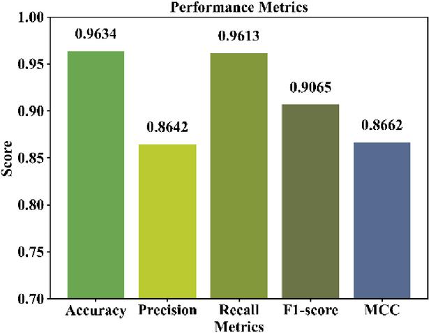
Figure 5 Performance metrics of the classification model.

The Figure 5 and Table 2 show the evaluation metrics such as Accuracy (0.9634), Precision (0.8642), Recall (0.9613), F1-score (0.9065), and MCC (0.8662). The high accuracy and recall indicate that the model is correctly identifying most of the instances with very few missed detections. The F1-score indicates that the model is in a good balance between precision and recall. Although the precision is slightly low compared to the recall, the high MCC indicates that the classification is highly reliable.

Table 2 Classification performance scores

Metrics	Values
Accuracy	0.9634
Precision	0.8642
Recall	0.9613
F1-score	0.9065
MCC	0.8662

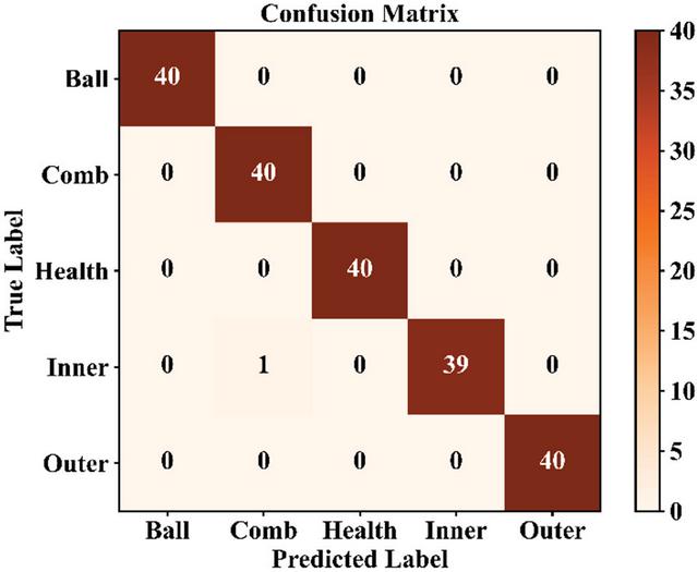
Figure 6 Confusion matrix.

The above confusion matrix displays the classification performance of the five different classes: Ball, Comb, Health, Inner, and Outer. The majority of the points are located along the diagonal of the matrix, representing accurate classification for all instances. The classes Ball, Comb, Health, and Outer each have 40 points correctly classified without any errors. The class Inner has 39 points correctly classified, and 1 of the points was misclassified as class Comb as shown in Figure 6. The confusion matrix provides detailed insight into the classification behavior of the proposed CNN–LSTM model across different fault categories. Most samples belonging to the Normal, Ball, and Outer race fault classes are correctly identified, indicating that the model effectively captures their distinguishing spatial and temporal characteristics. The Inner race fault category exhibits the highest classification difficulty, with a small number of samples being misclassified due to similarities in vibration patterns with other fault conditions. Despite this, the overall misclassification rate remains low, demonstrating the robustness of the proposed framework. The class-wise analysis confirms that the model maintains consistent predictive performance across multiple fault categories while preserving high fault detection reliability.

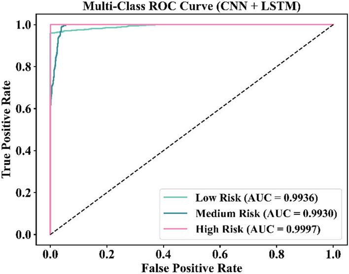
Figure 7 Multi-class ROC curve.

The above Figure 7 is a multi-class ROC for the classification of the model’s performance on the Low, Medium, and High classes. All three curves are near the top left corner of the graph, indicating the model’s classification capability is quite strong. The true positive rates are high, and the false positive rates are low. The AUC values are quite exceptional: 0.9936 for the Low-Risk class, 0.9930 for the Medium Risk class, and 0.9997 for the High Risk class. The High-Risk class’s discrimination is almost perfect. The ROC and Precision–Recall curves demonstrate the practical reliability of the proposed monitoring framework in operational hydropower environments. A high ROC-AUC value indicates that the model can effectively distinguish between healthy and faulty equipment conditions across different decision thresholds, thereby supporting reliable early warning generation. Similarly, the strong Precision–Recall performance confirms that most detected fault events correspond to actual equipment abnormalities, reducing the occurrence of false alarms that could trigger unnecessary inspections or maintenance actions. From an operational perspective, minimizing false positives improves maintenance efficiency and resource allocation, while maintaining high fault detection sensitivity ensures that potential equipment failures are identified before they escalate into critical safety incidents. Consequently, the observed ROC and Precision–Recall results indicate that the proposed CNN–LSTM framework is well suited for dependable early warning and safety monitoring in hydropower systems.

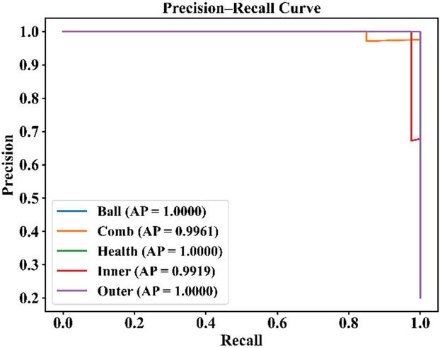
Figure 8 Precision-recall curve.

The precision-recall curve is used to measure the performance of the model for five classes, namely Ball, Comb, Health, Inner, and Outer. All the classes have near-perfect precision for most of the recall values, indicating that the model is making accurate predictions. The Average Precision (AP) values for the classes are extremely high, with Ball, Health, and Outer classes having an AP score of 1.0000. Although the AP score for the Comb class is 0.9961, and the score for the Inner class is 0.9919, the curves indicate that the model has performed extremely well in classification with minimal trade-offs between precision and recall as shown in Figure 8.

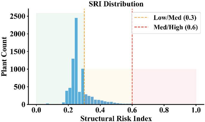
Figure 9 SRI distribution.

The above histogram represents the structural risk index distribution. The majority of plants are clustered between 0.15 and 0.30. The orange dashed line at 0.3 represents the boundary between low and medium structural risks. The red dashed line at 0.6 represents the boundary between medium and high structural risks. The majority of plants are clustered between 0.15 and 0.30, representing low structural risks. The overall distribution is right-skewed, suggesting that high-risk plants are fewer compared to low-risk plants as shown in Figure 9.

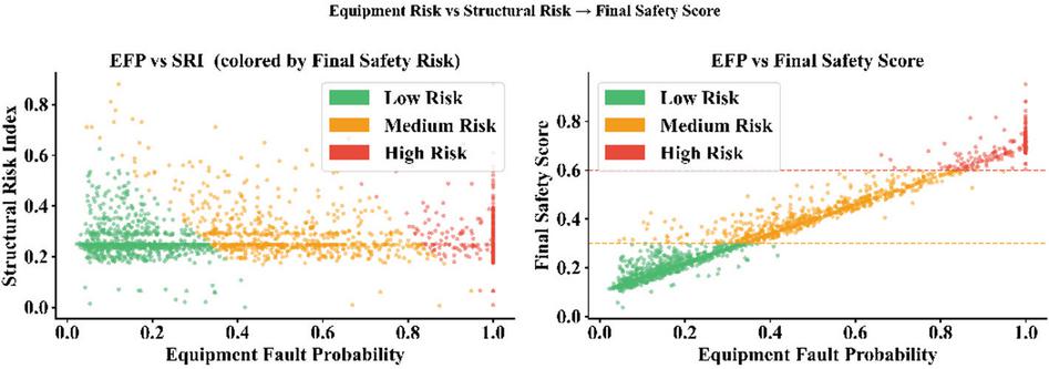
Figure 10 Equipment risk vs structural risk.

The Figure 10 displays a comparison of equipment fault probability and structural risk index with the final safety score. The left-hand plot demonstrates low risk points at lower values of equipment fault probability and structural risk index. The medium and high risk points are distributed over the higher equipment fault probability values. The right-hand plot displays a positive correlation between equipment fault probability and the final safety score. This suggests that equipment fault probability has a significant impact on the final safety score. It can be noted that equipment fault probability has a higher impact on the final safety score compared to structural risk index.

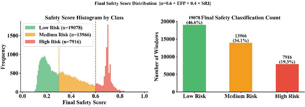
Figure 11 Final safety score distribution.

The above Figure 11 demonstrates the distribution and classification of the final safety scores calculated using the formula: $\alpha =0.6\ast \mathrm{EFP}+0.4\ast \mathrm{SRI}$. The histogram in the classification of samples into different risk categories based on the calculated safety scores. The risk categories are divided based on the warning threshold of 0.3 and the critical threshold of 0.6. The majority of the samples are classified as Low Risk, totaling 19,078 samples (46.6%), and have safety scores lower than 0.3. The Medium Risk category comprises 13,966 samples (34.1%), and the High-Risk category comprises 7,916 samples (19.3%), all of which have safety scores above the critical threshold of 0.6.

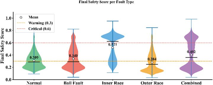
Figure 12 Final safety score per fault type.

This plot displays the distribution of the final safety scores for different types of faults, as represented by violin plots. The dashed lines for the warning level, represented by the dashed orange line, and the critical level, represented by the dashed red line, are 0.3 and 0.6, respectively. It is clear that the normal samples are concentrated below the warning level. For the Ball Fault and Outer Race, the distribution of the scores is more spread out, with some scores above the warning level. For the Inner Race Fault and Combined, the scores are more concentrated, indicating higher safety concerns as scores are near the critical level as shown in Figure 12.

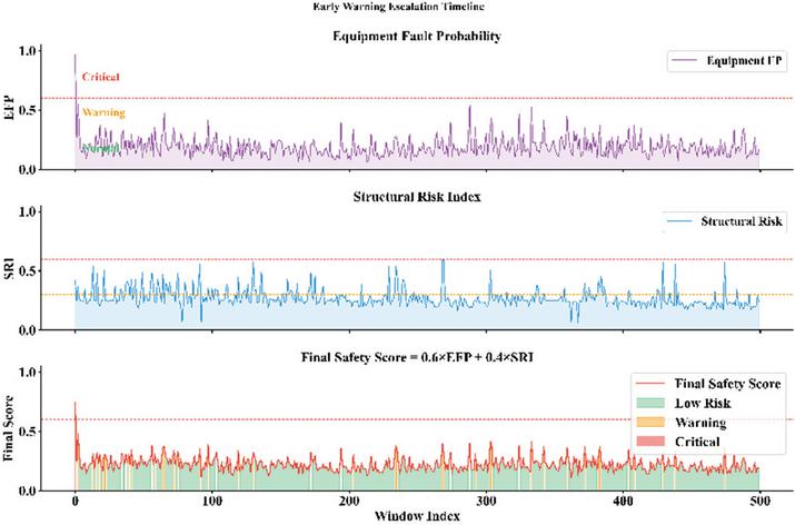
Figure 13 Early warning escalation timeline.

This early warning timeline displays equipment conditions through three important parameters: Equipment Fault Probability (EFP), Structural Risk Index (SRI), and the combined Final Safety Score. The EFP graph indicates fluctuations with occasional peaks approaching the warning threshold but remaining below it. The Final Safety Score combines these two parameters using the following equation: 0.6 * EFP $+$ 0.4 * SRI. The majority of its values lie within the low-risk zone with temporary excursions into the warning zone and very few instances in the critical zone as shown in Figure 13.

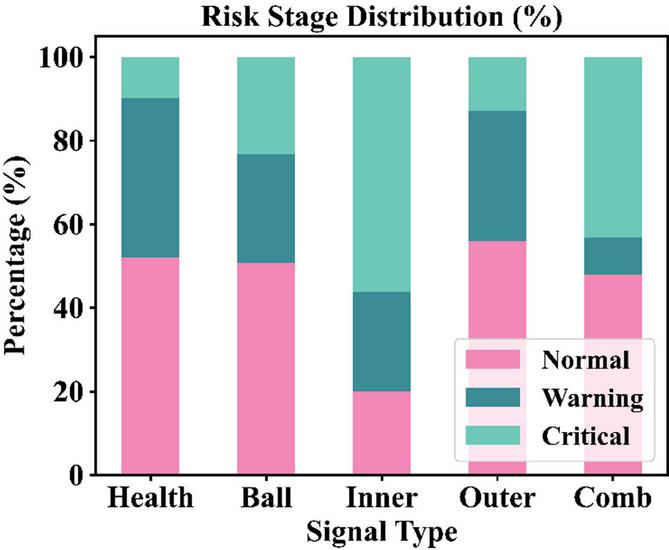
Figure 14 Risk stage distribution (%).

The chart illustrates the percentage distribution of the risk stages, which are Normal, Warning, and Critical. These stages are represented in different types of signals such as Health, Ball, Inner, Outer, and Combined. Based on the chart, the health and outer signals show the highest normal conditions. Therefore, these are the most stable in terms of performance. The Inner signal is the most critical since it shows the highest percentage in the Critical category. The Ball and Combined signals are balanced in terms of the number of conditions in the normal, warning, and critical stages as shown in Figure 14.

This dashboard represents the safety status of hydroponic equipment through key risk indicators. It indicates that the average health of the equipment is 0.435, and the average structural risk is 0.276. Thus, it concludes that the final safety score is 0.371. On the basis of this score, it is evident that the overall risk is Medium. The line chart represents how the safety score is changing during different monitoring windows. On the other hand, the risk counts chart represents that most of the windows represent low risk, followed by medium and high risks. It is recommended that the load should be reduced, maintenance should be done within 48 hours, and the next inspection should be done within 48 hours as shown in Figure 15.

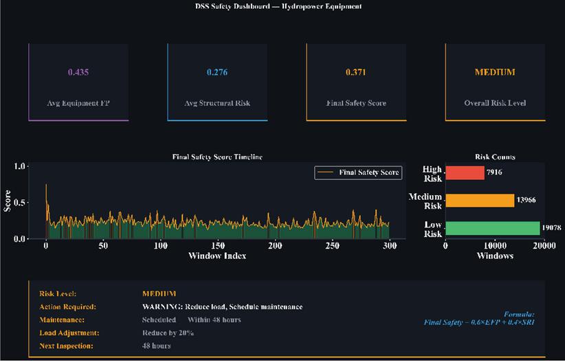
Figure 15 DSS safety dashboard.

This ablation study assesses the additional contribution of each component of the proposed model. Each CNN model and LSTM model represents the baseline performance of the model for fault detection. Using CNN and LSTM together with feature fusion improves accuracy, F1-score, and ROC-AUC. Adding structural risk information improves the model’s predictive power. The proposed model represents the best ROC-AUC and accuracy, validating the effectiveness of each component of the model as shown in Table 3.

Table 3 Ablation study of model variants for fault detection and risk assessment

Model Variant	Accuracy	F1-Score	ROC-AUC
CNN only	0.8630	0.8500	0.8800
LSTM only	0.8410	0.8300	0.8600
CNN-LSTM (no fusion)	0.8870	0.8700	0.9000
CNN-LSTM + Fusion	0.9190	0.9100	0.9300
Fusion + CNN-LSTM + Structural Risk	0.9340	0.9300	0.9500
Full Proposed Model	0.9634	0.9065	0.9905

Table 4 Comparative accuracy analysis of deep learning models for equipment fault diagnosis

Models	Accuracy
RNN [40]	0.9337
CNN [41]	0.9333
LSTM [42]	0.8613
Proposed Model	0.9634

6.1 Comparison with Other Models

Table 4 shows the comparative evaluation of the proposed model, namely CNN-LSTM, against existing deep learning techniques, as reported in recent literature. The traditional RNN model attained an accuracy of 0.9337, indicating moderate performance in sequential learning. However, it lacked the ability for spatial feature learning. Similarly, the proposed CNN model attained an accuracy of 93.33%, indicating its strong performance in spatial feature learning for the given vibration signals. Further, the proposed LSTM model attained an accuracy of 86.13%, indicating moderate performance in sequential learning. On the other hand, the proposed CNN-LSTM model attained the highest accuracy of 0.9634, indicating that the proposed model is effective in fault classification for hydropower equipment.

6.2 Discussion

The experimental results show that the proposed CNN-LSTM-based multi-source fusion framework can greatly improve the equipment-level health condition assessment performance compared to the single-model-based ones. The fusion of multi-channel vibration and torque signals can allow the model to learn both spatial fault signatures and temporal degradation patterns. Recent advancements in smart energy systems have demonstrated the effectiveness of digital twin technology for real-time energy management, monitoring, and optimization. Furthermore, the combination of graph convolutional networks and digital twin models has improved operational perception, network state assessment, and intelligent decision-making capabilities in distribution networks [43, 44]. This can improve the classification accuracy and stability of the model. It can be seen that the proposed CNN-LSTM-based multi-source fusion framework can better capture the progressive evolution of faults in rotating machinery systems compared to the performance of the single models. This verifies the effectiveness of the proposed framework in rotating machinery systems. The overall safety of a hydropower facility depends on the interaction between equipment health conditions and plant-level structural risk factors. Equipment health assessment provides information regarding the operational condition of critical assets such as turbines, generators, and associated rotating machinery, whereas the Structural Risk Index (SRI) reflects broader infrastructure-related risks associated with dam characteristics, reservoir capacity, and plant configuration.

Apart from equipment-level monitoring, the addition of structural information related to the plant-level variables from the GloHydroRes dataset helps to improve the overall safety evaluation process. This is done by moving from a fault-detection approach to a more risk-conscious approach through a hierarchical fusion of dam height, reservoir volume, capacity, and type of plants in a structural risk index model. This hierarchical approach helps to distinguish between similar types of equipment faults that have occurred under different structural or risk conditions. This leads to a more holistic safety score that represents a higher level of overall operation risks.

The decision support system takes the predictive results and turns them into recommendations, which is another aspect of practical application of the results in real-world hydropower settings. By relating fault probability and structural risk to warning levels, the proposed framework eliminates confusion that may occur when interpreting alarm messages. Although the study is comprehensive, it is limited by its use of laboratory data from rotating machinery for validation of the proposed framework, which should be replaced with real-world hydropower SCADA data. Validation of the proposed framework using real-world turbine generator data is recommended for future work, along with consideration of hydrological and climate variability factors for improved safety predictions.

7 Conclusion and Future Works

The research proposed a framework for multi-level health condition assessment and safety early warning, which combines a CNN-LSTM model for equipment fault diagnosis and a structural risk evaluation model at the plant level. The performance of the proposed model has been verified through experiments using the multi-sensor dataset from SEU. The proposed model has demonstrated good performance with high Accuracy: 0.9634, Precision: 0.8642, Recall: 0.9613, F1-score: 0.9065, and Matthews Correlation Coefficient: 0.8662. The confusion matrix has further verified that the proposed model has high reliability with only one misclassification from the Inner race fault class. The multi-class ROC has further verified the robustness of the proposed model with high AUC values: 0.9936 for Low Risk, 0.9930 for Medium Risk, and 0.9997 for High Risk. The Precision-Recall curves further verified that the proposed model has high Average Precision with high values: 1.0000 for Ball, Health, and Outer.

At the plant level, the result of the Structural Risk Index (SRI) analysis showed that the majority of the hydropower plants fell in the range of 0.15–0.30. These values corresponded to low structural risk conditions. Finally, the distribution of the unified safety score, which included the Equipment Fault Probability (EFP) and the Structural Risk Index (SRI), revealed the following final result: 46.6% Low Risk (19,078 samples), 34.1% Medium Risk (13,966 samples), and 19.3% High Risk (7,916 samples). The result of the analysis showed that the equipment fault probability played a more important role in the final safety score than the structural risk.

Future Works

• Test the developed model with real SCADA data from a hydropower plant instead of laboratory data to evaluate the performance of the model.

• Instead of using weights, use adaptive or optimized weighting methods to improve the accuracy of the risk calculation.

• Include hydrological and environmental factors along with weather conditions to improve the accuracy of structural risk prediction.

Declarations

Data Availability

The datasets used in this study include the SEU multi-sensor dataset and the GloHydroRes dataset, which are publicly available from their respective repositories. Additional data supporting the findings of this study are available from the corresponding author upon reasonable request.

Conflicts of Interest/Competing Interests

The authors declare that they have no competing interests.

Funding

this work was funded by 2025 Fujian Huadian Furui Energy Development Co., Ltd. Technology Project: Research and Application of Regional Equipment Full Lifecycle Management Based on Information Technology Innovation, Project No.: CHDKJ24-04-02-445

Author Contributions

Qiaofeng Lin: Conceptualization, methodology, software, data analysis, writing—original draft. Shijian Wu: Supervision, validation, writing—review and editing.

Ethical Approval

This article does not contain any studies involving human participants or animals performed by any of the authors.

Consent to Participate

Not applicable.

Consent to Publication

The authors consent to the publication of this manuscript.

References

[1] Su Y, Gan H, Ji Z (2024) Research on multi-parameter fault early warning for marine diesel engine based on PCA-CNN-BiLSTM. J Mar Sci Eng 12:965. https://doi.org/10.3390/jmse12060965.

[2] He X et al. (2023) Situation awareness of energy internet of things in smart city based on digital twin: from digitization to informatization. IEEE Internet Things J 10(9):7439–7458. https://doi.org/10.1109/JIOT.2022.3203823.

[3] Lu J et al. (2025) Multi-modal intelligent fault detection of screening equipment using sparse sensing and deep visual analysis: field application in coal preparation plants. Int J Coal Prep Util: 1–28. https://doi.org/10.1080/19392699.2025.2584172.

[4] Wang Z, Wang S, Chen Y, Zhan M, Wang Y, Sun C (2025) A pattern-guided CIM vulnerability diagnosis framework for multi-sensor thermal management system in energy storage stations. Energies 18:6158. https://doi.org/10.3390/en18236158.

[5] Peng J (2025) Digital twin technology and its application in water governance: China’s practices and achievements. Int J Water Resour Dev 41(5–6):974–989. https://doi.org/10.1080/07900627.2025.2544810.

[6] Wu X et al. (2025) From forecasting to foresight: building an autonomous O&M brain for the new power system based on a cognitive digital twin. Electronics 14:4537. https://doi.org/10.3390/electronics14224537.

[7] Tang T, Zhao C, Liu X, Sun S (2025) Digital twin-enabled deep learning for real-time fire situation awareness. Vis Comput 41(14):11857–11869. https://doi.org/10.1007/s00371-025-04131-0.

[8] Wei A, Ke H, He S, Jiang M, Yao Z, Yi J (2025) Enhanced landslide risk evaluation in hydroelectric reservoir zones utilizing an improved random forest approach. Water 17:946. https://doi.org/10.3390/w17070946.

[9] Dui H, Dong X, Wu X, Chen L, Bai G (2024) IoT-enabled risk warning and maintenance strategy optimization for tunnel-induced ground settlement. IEEE Internet Things J 11(13):22966–22981. https://doi.org/10.1109/JIOT.2024.3377440.

[10] Zou Y et al. (2025) Multi-stakeholder risk assessment of a waterway engineering project during the decision-making stage from the perspective of sustainability. Sustainability 17:5372. https://doi.org/10.3390/su17125372.

[11] Ahmed S, Alnaqbi AH, Al Hemairy M, Al Ahmad M (2018) ECG abnormality detection algorithm. Int J Adv Comput Sci Appl 9(8):215–221. https://doi.org/10.14569/ijacsa.2018.090827.

[12] Al Hemairy M, Amin S, Hijji M, Serhani M, Al Ahmad M (2016) Integrated and scalable architecture for providing cost-effective remote health monitoring. In: Proc 9th Int Conf Dev eSystems Eng (DeSE), pp. 74–77. https://doi.org/10.1109/DeSE.2016.14.

[13] Zhang P, Wang Q, Xu S, Zhu J, Zhong S, Zhang Y (2025) Early warning of coal mine production environment safety risks based on multi-source information feature fusion. Sustainability 17:2085. https://doi.org/10.3390/su17052085.

[14] Plakantara SP, Karakitsiou A (2025) Transforming agrifood supply chains with digital technologies: a systematic review of safety and quality risk management. Oper Res Forum 6:113. https://doi.org/10.1007/s43069-025-00511-3.

[15] Jiaxiang O et al. (2025) Intelligent hardware design for wire status monitoring integrating Beidou GNSS and inertial measurement technology in machine learning environment. Aust J Electr Electron Eng 22(4):575–586. https://doi.org/10.1080/1448837X.2024.2423982.

[16] Li H, Zhao H, Shen Y, Zheng S, Zhang R (2024) Structural health monitoring and failure analysis of large-scale hydro-steel structures based on multi-sensor information fusion. Water 16:3167. https://doi.org/10.3390/w16223167.

[17] Feng Z, Liang Q, Wei M, Li L, Bu Y, Xin Y (2025) Management system and optimal control for three-dimensional visualization and maintenance of thermal power plant. Energy Inform 8:71. https://doi.org/10.1186/s42162-025-00491-y.

[18] Xin L, Zhao Y, Zhao Q (2025) BeiDou and SAR fusion technology with AI in reservoir dam monitoring for climate-based disaster mitigation. Discov Artif Intell 5:100. https://doi.org/10.1007/s44163-025-00320-x.

[19] Shao S, Zhou F, Wang Y, Wu J (2025) An integrated multi-sensor information system for real-time reservoir monitoring and management. Sensors 25:5730. https://doi.org/10.3390/s25185730.

[20] Sun J, Fei L (2025) A generative AI-enhanced case-based reasoning method for risk assessment: ontology modeling and similarity calculation framework. Mathematics 13:2735. https://doi.org/10.3390/math13172735.

[21] Bai J et al. (2024) Fault diagnosis of pumped storage units—a novel data-model hybrid-driven strategy. Processes 12:2127. https://doi.org/10.3390/pr12102127.

[22] Zhou X et al. (2025) A fault diagnosis method for centrifugal compressors based on ontology and Bayesian network fusion reasoning. Concurr Comput Pract Exp 37:e70278. https://doi.org/10.1002/cpe.70278.

[23] Li S et al. (2025) Key technologies and applications of digital twin hydraulic engineering. Digit Twin 2:2486862. https://doi.org/10.1080/27525783.2025.2486862.

[24] Xie Y, Zeng W, Qiu J (2023) Integrated water risk early warning framework of the semi-arid transitional zone based on the water environmental carrying capacity (WECC). J Arid Land 15(2):145–163. https://doi.org/10.1007/s40333-022-0083-z.

[25] Zhao T et al. (2025) Leveraging immersive digital twins and AI-driven decision support systems for sustainable water reserves management: a conceptual framework. Sustainability 17:3754. https://doi.org/10.3390/su17083754.

[26] Negi P et al. (2024) Specific soft computing strategies for the digitalization of infrastructure and its sustainability: a comprehensive analysis. Arch Comput Methods Eng 31(3):1341–1362. https://doi.org/10.1007/s11831-023-10018-x.

[27] Liu H, Su H, Li H (2024) Study on digital twin technologies for watershed information modeling (WIM): a systematic literature review and bibliometric analysis. Arch Comput Methods Eng 31(1):263–289. https://doi.org/10.1007/s11831-023-09977-y.

[28] Ling M et al. (2025) Framework for comprehensive risk assessment and factor diagnosis from the perspective of the water–energy–food–ecology–carbon complex system: a case study of the Yellow River ‘Ji’ Bay. Sustainability 17:9637. https://doi.org/10.3390/su17219637.

[29] Ma L, Chen S, Wei D, Zhang Y, Guo Y (2024) A comprehensive hybrid deep learning approach for accurate status predicting of hydropower units. Appl Sci 14:9323. https://doi.org/10.3390/app14209323.

[30] Zhang L, Hou Y, Deng K, Xin J (2025) Advancements toward a standard system for intelligent operation and maintenance of buildings and municipal facilities. Buildings 15:3965. https://doi.org/10.3390/buildings15213965.

[31] Zhao J et al. (2025) Analysis of construction safety risk management for cold region concrete gravity dams based on fuzzy VIKOR-LEC. Buildings 15:1981. https://doi.org/10.3390/buildings15121981.

[32] Zhang W, Meng H, Wang R, Wang P (2025) Intelligent optimized diagnosis for hydropower units based on CEEMDAN combined with RCMFDE and ISMA-CNN-GRU-attention. Water 17:2125. https://doi.org/10.3390/w17142125.

[33] Liu G et al. (2025) Advances in artificial intelligence and digital twin for tunnel boring machines. Artif Intell Rev 58:257. https://doi.org/10.1007/s10462-025-11261-3.

[34] Tian J, Zhang X, Zheng S, Liu Z, Zhan C (2024) Synergising an advanced optimisation technique with deep learning: a novel method in fault warning systems. Mathematics 12:1301. https://doi.org/10.3390/math12091301.

[35] Zhou Y et al. (2025) IoT-driven intelligent curing of face slab concrete in rockfill dams based on integrated multi-source monitoring. Buildings 15:2344. https://doi.org/10.3390/buildings15132344.

[36] Pi Y, Tan Y, Golmohammadi AM, Guo Y, Xiao Y, Chen Y (2023) A fault warning approach using an enhanced sand cat swarm optimization algorithm and a generalized neural network. Processes 11:2543. https://doi.org/10.3390/pr11092543.

[37] Zhang S, Liu J, Li Z, Xiahou X, Li Q (2024) Analyzing critical factors influencing the quality management in smart construction site: a DEMATEL-ISM-MICMAC based approach. Buildings 14:2400. https://doi.org/10.3390/buildings14082400.

[38] cathysiyu (2026) Mechanical-datasets/gearbox/gearset. GitHub. Available at: https://github.com/cathysiyu/Mechanical-datasets/tree/master/gearbox/gearset (Accessed 24 Feb 2026)

[39] Shah J, Hu J, Edelenbosch O, van Vliet MTH (2024) GloHydroRes—a global dataset combining open-source hydropower plant and reservoir data. Zenodo. https://doi.org/10.5281/zenodo.14526360.

[40] Liu B, Wang X, Zhang Z, Zhao Z, Wang X, Liu T (2025) Fault prediction of hydropower station based on CNN-LSTM-GAN with biased data. Energies 18:3772. https://doi.org/10.3390/en18143772.

[41] Yang Z et al. (2025) Hybrid CNN-BiLSTM-MHSA model for accurate fault diagnosis of rotor motor bearings. Mathematics 13:334. https://doi.org/10.3390/math13030334.

[42] Han K, Wang W, Guo J (2024) Research on a bearing fault diagnosis method based on a CNN-LSTM-GRU model. Machines 12:927. https://doi.org/10.3390/machines12120927.

[43] He X (2026) Digital twin-enabled smart energy management for mega sports events. Distrib Gener Altern Energy J 41(2):245–270.

[44] Liu Y, Bai H, Li W (2026) A distribution network operational situation perception technology based on graph convolutional neural network-enhanced digital twin model. Distrib Gener Altern Energy J 41(2):301–326.

Biographies

Qiaofeng Lin obtained his Bachelor’s degree from Nanchang Institute of Technology in 2013. He has been working at Fujian Branch of China Huadian Corporation since 2021. He has received honors including Advanced Individual in Work Safety, Outstanding Young Post Expert of Fujian Province, and National Young Post Expert. He specializes in hydraulic mechanical engineering and hydropower station operation, and has published 6 academic papers.

Shijian Wu received his Bachelor’s degree from Huaqiao University in 2009. He has been working at China Huadian Corporation Fujian Branch since 2009. In 2014, he was awarded the Bronze Award for Excellent Achievements in the 3rd Youth Innovation & Efficiency Competition of China Huadian Corporation for the “Kemen 7S Coal Unloading Method”. He specializes in project management and procurement management, and has authored and published more than 10 academic papers.

Distributed Generation & Alternative Energy Journal, Vol. 41_5, 1241–1298
doi: 10.13052/dgaej2156-3306.4153
© 2026 River Publishers