Meshfree Galerkin Method for a Rotating Non-Uniform Rayleigh Beam with Refinement of Radial Basis Functions

Vijay Panchore

Maulana Azad National Institute of Technology, Mechanical Engineering, Bhopal, 462003, India

E-mail: vijaypanchore36@gmail.com

Received 16 August 2021; Accepted 04 January 2022; Publication 19 January 2022

Abstract

The rotating Rayleigh beam problem is solved with meshfree method where the radial basis functions are explored. Numbers of basis functions have been used for meshfree methods which also include radial basis function. In this paper, the Gaussian radial basis function and multiquadrics radial basis functions are combined to get the new basis function which provides accuracy for higher natural frequencies. The radial basis functions satisfy the Kronecker delta property and it is easy to apply the essential boundary conditions. The Galerkin method is used for weak formulation. The matrices have been derived. The results are obtained for Gaussian radial basis function and new basis function. The results show more accurate values for fourth and fifth natural frequency with new basis function where only six nodes are used within the subdomain of trial and test function. The results are also obtained with conventional finite element method where forty, two node elements are considered. Also, the results are obtained for rotating Euler-Bernoulli beam to observe the difference in results with rotating Rayleigh beam.

Keywords: Galerkin method, Gaussian radial basis function, multiquadrics radial basis function, rotating beam, free vibration, meshfree methods.

1 Introduction

The meshfree methods are based on nodal approximation when compared to element approximation of conventional finite element method. The radial basis functions and moving least squares approximations are mostly used for deriving the shape functions [1, 2]. The radial basis functions can further be divided: (1)  Thin plate splines radial basis function, (2) Multiquadrics radial basis function, (3) Gaussian radial basis function and (4) logarithmic radial basis function [1]. To develop the new basis function with higher accuracy we can refine the different approximations for radial basis functions. This area of meshfree approximation can be explored to get new solutions based on the structure of problem. The weak formulation for the problem can be developed based on the subdomain of test and trial function.

The weak form can be obtained with collocation method and Galerkin method. These methods differ from the Meshless Petrov-Galerkin method where algebraic equations can be written for each node. In Galerkin method the trial and test function have the same subdomain. The number of nodes within the subdomain can be considered based on the matrices which have to be inverted. The meshless Galerkin method has been used to solve Dirichlet boundary value problems where radial basis functions are considered [3]. Also, the radial basis functions are explored where Galerkin method is considered for the weak form [4]. The collocation method is used to solve Burgers’ equation where the method is found to be accurate for high Reynolds number [5]. A meshless approach has been used for the bimodulus materials, the method found to be highly accurate and convergent [6]. The Rayleigh beam theory, which provides a single differential equation, has been solved with spinning and axial motions for vibration problem [7].

The rotating beam problems, which include an additional centrifugal force when compared to non-rotating beams, have been solved with conventional finite element method [8–11]. These methods include Galerkin and collocation approaches where different derived basis functions are used [12–14]. Mesh free method has been used to Euler-Bernoulli beam problem using radial basis function [2]. The rotating beam problems: Rayleigh beam, Timoshenko beam and Euler-Bernoulli beam have been solved in literature using meshless Petrov-Galerkin method and B-spline finite element method [15–17]. The tapered rotating Euler-Bernoulli beam problem has been solved with Adomian decomposition method [18]. Spectral finite element method is used to solve the rotating beam problem as well [19]. The semi analytical solutions are obtained for rotating beam where series solutions are explored with Frobenius method [20]. The problem of rotating functionally graded beams is solved for steady bending deformation [21].

The complete formulation for a rotating beam problem subjected to an aerodynamic force has been discussed where finite element in time and stability of the system are explained as well [22]. Many possible formulations are discussed in literature and the results have been obtained with numbers of basis functions [23]. The mass and stiffness matrices have been derived where symmetric stiffness matrix formulation has been obtained with Galerkin method for the first time [24]. For Euler-Bernoulli, Timoshenko and Rayleigh beams the matrices have been derived and solved with conventional methods. A rotating Timoshenko beam theory, which results in two coupled equations, has a shear locking problem which can be solved with radial basis function approximation [16]. The results of all these rotating beams are compared in the literature as well. In rotating beam literature, the rotating Rayleigh beam problem has not been explored with meshless Galerkin method and with refined radial basis functions.

In this paper, we solve the rotating Rayleigh beam problem using meshless Galerkin method where radial basis functions are considered as basis functions. Two types of radial basis functions, Gaussian and multiquadrics, are multiplied together to form a new radial basis function which provides better results for fourth and fifth natural frequencies when compared to Gaussian alone. The multiquadrics radial basis functions are refined and Gaussian radial basis functions are kept same before the multiplication. The results have been verified from the literature [25]. The results are accurate when only six nodes are considered in the subdomain of trial and test function. Above six nodes the ill conditioning of matrices occurs. The results are obtained for non-uniform, non-rotating beam as well. Also, the results are obtained for the rotating Euler-Bernoulli beams and compared with Rayleigh beam. All the matrices have been derived, the natural boundary conditions are satisfied by integrating the weak form and essential boundary conditions are applied in matrix form.

2 Weak Formulation of the Governing Differential Equation

The governing differential equation of a rotating Rayleigh beam is given by

${\displaystyle \frac{{\partial }^2}{\partial x^2}}\left[EI(x){\displaystyle \frac{{\partial }^{2}w(x,t)}{\partial x^2}}\right]+\rho A(x){\displaystyle \frac{{\partial }^{2}w(x,t)}{\partial t^2}}-{\displaystyle \frac{\partial }{\partial x}}\left[G(x){\displaystyle \frac{\partial w(x,t)}{\partial x}}\right]$
$\mathrm{\hspace{1em}\hspace{1em}}+{\displaystyle \frac{\partial }{\partial x}}\left\{\rho I(x){\displaystyle \frac{\partial }{\partial x}}\left[{\mathrm{\Omega }}^{2}w(x,t)-{\displaystyle \frac{{\partial }^{2}w(x,t)}{\partial t^2}}\right]\right\}=0$	(1)

The fourth term is an additional term when compared to Euler-Bernoulli beam theory. This includes additional rotary inertia. Here, the flexural stiffness is $EI(x)$, density is $\rho$, cross sectional area is $A(x)$, transverse displacement is $w(x)$ and $G(x)$ is the centrifugal force which is given by

$$G(x)={\int }_x^R\rho A(x){\mathrm{\Omega }}^{2}x\mathit{d}x$$

(2)

where, $\mathrm{\Omega }$ is angular velocity and $R$ is radius of the rotating beam.

After substituting $w(x,t)=e^{i\omega t}\overline{w}(x),$ we get the free vibration problem of a rotating beam which is given by

${\displaystyle \frac{d^2}{d{x}^2}}\left[EI(x){\displaystyle \frac{d^2\overline{w}(x)}{d{x}^2}}\right]-{\omega }^2\rho A(x)\overline{w}(x)-{\displaystyle \frac{d}{dx}}\left[G(x){\displaystyle \frac{d\overline{w}(x)}{dx}}\right]$
$\mathrm{\hspace{1em}\hspace{1em}}+{\displaystyle \frac{d}{dx}}\left\{\rho I(x){\displaystyle \frac{d}{dx}}\left[({\mathrm{\Omega }}^2+{\omega }^2)\overline{w}(x)\right]\right\}=0$	(3)

The weak form of Equation (3) is given by

${\displaystyle {\int }_0^R}v(x)\left\{{\displaystyle \frac{d^2}{d{x}^2}}\left[EI(x){\displaystyle \frac{d^2\overline{w}(x)}{d{x}^2}}\right]-\rho A(x){\omega }^2\overline{w}(x)-{\displaystyle \frac{d}{dx}}\left[G(x){\displaystyle \frac{d\overline{w}(x)}{dx}}\right]\right\}\mathit{d}x$
$\mathrm{\hspace{1em}\hspace{1em}}+{\displaystyle {\int }_0^R}v(x){\displaystyle \frac{d}{dx}}\left\{\rho I(x){\displaystyle \frac{d}{dx}}\left[\left({\mathrm{\Omega }}^2+{\omega }^2\right)\overline{w}(x)\right]\right\}=0$	(4)

Integrating Equation (4) by parts, we get

${\left|v(x)\left\{{\displaystyle \frac{d}{dx}}\left[EI(x){\displaystyle \frac{d^2\overline{w}(x)}{d{x}^2}}\right]-G(x){\displaystyle \frac{d\overline{w}(x)}{dx}}+\rho I(x){\displaystyle \frac{d}{dx}}\left[({\mathrm{\Omega }}^2+{\omega }^2)\overline{w}(x)\right]\right\}\right|}_0^R$
$\mathrm{\hspace{1em}\hspace{1em}}-{\left|{\displaystyle \frac{dv(x)}{dx}}EI(x){\displaystyle \frac{d^2\overline{w}(x)}{d{x}^2}}\right|}_0^R+{\displaystyle {\int }_0^R}EI(x){\displaystyle \frac{d^{2}v(x)}{d{x}^2}}{\displaystyle \frac{d^2\overline{w}(x)}{d{x}^2}}\mathit{d}x$
$\mathrm{\hspace{1em}\hspace{1em}}+{\displaystyle {\int }_0^R}G(x){\displaystyle \frac{dv(x)}{dx}}{\displaystyle \frac{d\overline{w}(x)}{dx}}\mathit{d}x-{\mathrm{\Omega }}^2{\displaystyle {\int }_0^R}\rho I(x){\displaystyle \frac{dv(x)}{dx}}{\displaystyle \frac{d\overline{w}(x)}{dx}}\mathit{d}x$
$\mathrm{\hspace{1em}\hspace{1em}}-{\omega }^2{\displaystyle {\int }_0^R}\rho A(x)v(x)\overline{w}(x)\mathit{d}x-{\omega }^2{\displaystyle {\int }_0^R}\rho I(x){\displaystyle \frac{dv(x)}{dx}}{\displaystyle \frac{d\overline{w}(x)}{dx}}\mathit{d}x=0$	(5)

Here the test function satisfies the essential boundary conditions. The natural boundary conditions, which are shear force and bending moment at the tip, are satisfied as well, which are given by Equations (6) and (7)

$\{{\displaystyle \frac{d}{dx}}\left[EI(x){\displaystyle \frac{d^2\overline{w}(x)}{d{x}^2}}\right]-G(x){\displaystyle \frac{d\overline{w}(x)}{dx}}$
$\mathrm{\hspace{1em}\hspace{1em}}+\rho I(x){\displaystyle \frac{d}{dx}}[({\mathrm{\Omega }}^2+{\omega }^2)\overline{w}(x)]\left\}\right|{}_{(x=R)}=0$	(6)
${EI(x){\displaystyle \frac{d^2\overline{w}(x)}{d{x}^2}}|}_{(x=R)}=0$	(7)

Equation (5) now can be rewritten as

${\displaystyle {\int }_0^R}EI(x){\displaystyle \frac{d^{2}v(x)}{d{x}^2}}{\displaystyle \frac{d^2\overline{w}(x)}{d{x}^2}}\mathit{d}x+{\displaystyle {\int }_0^R}G(x){\displaystyle \frac{dv(x)}{dx}}{\displaystyle \frac{d\overline{w}(x)}{dx}}\mathit{d}x$
$\mathrm{\hspace{1em}\hspace{1em}}-{\mathrm{\Omega }}^2{\displaystyle {\int }_0^R}\rho I(x){\displaystyle \frac{dv(x)}{dx}}{\displaystyle \frac{d\overline{w}(x)}{dx}}\mathit{d}x-{\omega }^2{\displaystyle {\int }_0^R}\rho A(x)v(x)\overline{w}(x)\mathit{d}x$
$\mathrm{\hspace{1em}\hspace{1em}}-{\omega }^2{\displaystyle {\int }_0^R}\rho I(x){\displaystyle \frac{dv(x)}{dx}}{\displaystyle \frac{d\overline{w}(x)}{dx}}\mathit{d}x-0$	(8)

The conventional finite element assumption is given by Equations (9) and (10)

$\overline{w}(x)$	$=[N(x)][q]$	(9)
$v(x)$	$={[\delta q]}^T{[N(x)]}^T$	(10)

From Equations (8), (9) and (10), we write

$[{\displaystyle {\int }_0^R}EI(x){\displaystyle \frac{d^2{[N]}^T}{d{x}^2}}{\displaystyle \frac{d^2[N]}{d{x}^2}}dx+{\displaystyle {\int }_0^R}G(x){\displaystyle \frac{d{[N]}^T}{dx}}{\displaystyle \frac{d[N]}{dx}}dx$
$\mathrm{\hspace{1em}\hspace{1em}}-{\mathrm{\Omega }}^2{\displaystyle {\int }_0^R}\rho I(x){\displaystyle \frac{d{[N]}^T}{dx}}{\displaystyle \frac{d[N]}{dx}}][q]$
$\mathrm{\hspace{1em}\hspace{1em}}-\left[{\omega }^2{\displaystyle {\int }_0^R}\rho A(x){[N]}^T[N]\mathit{d}x+{\omega }^2{\displaystyle {\int }_0^R}\rho I(x){\displaystyle \frac{d{[N]}^T}{dx}}{\displaystyle \frac{d[N]}{dx}}\mathit{d}x\right][q]=0$	(11)

where, $[N(x)]$ represents the shape function vector and $[q]$ represents a vector containing nodal degrees of freedom.

Here, the stiffness matrix is given by

$[K]={\displaystyle {\int }_0^R}EI(x){\displaystyle \frac{d^2{[N]}^T}{d{x}^2}}{\displaystyle \frac{d^2[N]}{d{x}^2}}\mathit{d}x+{\displaystyle {\int }_0^R}G(x){\displaystyle \frac{d{[N]}^T}{dx}}{\displaystyle \frac{d[N]}{dx}}\mathit{d}x$
$\mathrm{\hspace{1em}\hspace{1em}}-{\mathrm{\Omega }}^2{\displaystyle {\int }_0^R}\rho I(x){\displaystyle \frac{d{[N]}^T}{dx}}{\displaystyle \frac{d[N]}{dx}}$	(12)

and the mass matrix is given by

$[M]={\displaystyle {\int }_0^R}\rho A(x){[N]}^T[N]\mathit{d}x+{\displaystyle {\int }_0^R}\rho I(x){\displaystyle \frac{d{[N]}^T}{dx}}{\displaystyle \frac{d[N]}{dx}}\mathit{d}x$

(13)

The relative stiffness and mass matrix of an Euler-Bernoulli beam is given by Equations (14) and (15)

${[K]}_{E-B}$	$={\displaystyle {\int }_0^R}EI(x){\displaystyle \frac{d^2{[N]}^T}{d{x}^2}}{\displaystyle \frac{d^2[N]}{d{x}^2}}\mathit{d}x+{\displaystyle {\int }_0^R}G(x){\displaystyle \frac{d{[N]}^T}{dx}}{\displaystyle \frac{d[N]}{dx}}\mathit{d}x$ (14)
${[M]}_{E-B}$	$={\displaystyle {\int }_0^R}\rho A(x){[N]}^T[N]\mathit{d}x$	(15)

Finally, the eigenvalue problem can be solved to get the natural frequencies and mode shapes which is given by

$${\omega }^2[M][\varphi ]=[K][\varphi ]$$

(16)

Where, $i=1,2,3\mathrm{\dots }N,$ where, ${\omega }_1$ is the first natural frequency and $[\varphi ]$ is an eigenvector.

3 Rotating Rayleigh Beam Equation in Non-dimensional Form

The equations can be written in non-dimensional form where the term are given by [25]

$I(x)=I_{0}g(x),A(x)=A_{0}f(x)$

(17,18)

Here,

$g(x)={\left(1-c{\displaystyle \frac{x}{R}}\right)}^{\overline{n}+2},f(x)={\left(1-c{\displaystyle \frac{x}{R}}\right)}^{\overline{n}}$

(19,20)

and $c$ is a constant. Here, $A_0$ and $I_O$ are the constant cross sectional area and second moment of area terms, respectively.

The Equation (3) can be written in non-dimensional form as

${\displaystyle \frac{d^2}{d{\zeta }^2}}\left[g(\zeta ){\displaystyle \frac{d^2\overline{w}(\zeta )}{d{\zeta }^2}}\right]-{\lambda }^{2}f(\zeta )\overline{w}(\zeta )-s^2{\displaystyle \frac{d}{d\zeta }}\left[h(\zeta ){\displaystyle \frac{d\overline{w}(\zeta )}{d\zeta }}\right]$
$\mathrm{\hspace{1em}\hspace{1em}}+{\displaystyle \frac{s^2}{r^2}}{\displaystyle \frac{d}{d\zeta }}\left[g(\zeta ){\displaystyle \frac{d\overline{w}(\zeta )}{d\zeta }}\right]+{\displaystyle \frac{{\lambda }^2}{r^2}}{\displaystyle \frac{d}{d\zeta }}\left[g(\zeta ){\displaystyle \frac{d\overline{w}(\zeta )}{d\zeta }}\right]=0$	(21)

where,

$$\zeta =\frac{x}{R},r^2=\frac{A_0{R}^2}{I_0},s^2={\mathrm{\Omega }}^2\frac{\rho A_0{R}^4}{E{I}_0},{\lambda }^2={\omega }^2\frac{\rho A_0{R}^4}{E{I}_0},$$

$$\text{and}\mathit{\hspace{1em}}h(\zeta )={\int }_{\zeta }^1\zeta f(\zeta )\mathit{d}\zeta .$$

Here, $s$ and $\lambda$ are the non-dimensional rotating speed and natural frequency respectively and $r$ is the slenderness ratio.

The essential and natural boundary conditions are given by

${\overline{w}(\zeta )|}_{(\zeta =0)}=0,{{\displaystyle \frac{d\overline{w}(\zeta )}{d\zeta }}|}_{(\zeta =0)}=0,$

(22,23)

$\{{\displaystyle \frac{d}{d\zeta }}\left[g(\zeta ){\displaystyle \frac{d^2\overline{w}(\zeta )}{d{\zeta }^2}}\right]-s^{2}h(\zeta ){\displaystyle \frac{d\overline{w}(\zeta )}{d\zeta }}$
$\mathrm{\hspace{1em}\hspace{1em}}+{\displaystyle \frac{(s^2+{\lambda }^2)}{r^2}}g(\zeta ){\displaystyle \frac{d\overline{w}(\zeta )}{d\zeta }}\left\}\right|{}_{(x=R)}=0$	(24)
${g(\zeta ){\displaystyle \frac{d^2\overline{w}(\zeta )}{d{\zeta }^2}}|}_{(x=R)}=0$	(25)

Weak formulation of Equation (21) gives the stiffness and mass matrices as

$[K]$	$={\displaystyle {\int }_0^1}g(\zeta ){\displaystyle \frac{d^2{[N]}^T}{d{\zeta }^2}}{\displaystyle \frac{d^2[N]}{d{\zeta }^2}}\mathit{d}\zeta +{\displaystyle {\int }_0^1}{s}^{2}h(\zeta ){\displaystyle \frac{d{[N]}^T}{d\zeta }}{\displaystyle \frac{d[N]}{d\zeta }}\mathit{d}\zeta$
	$\mathrm{\hspace{1em}\hspace{1em}}-{\displaystyle {\int }_0^1}{\displaystyle \frac{s^2}{r^2}}g(\zeta ){\displaystyle \frac{d{[N]}^T}{d\zeta }}{\displaystyle \frac{d[N]}{d\zeta }}\mathit{d}\zeta$	(26)
$[M]$	$={\displaystyle {\int }_0^1}f(\zeta ){[N]}^T[N]\mathit{d}\zeta +{\displaystyle {\int }_0^1}{\displaystyle \frac{1}{r^2}}g(\zeta ){\displaystyle \frac{d{[N]}^T}{d\zeta }}{\displaystyle \frac{d[N]}{d\zeta }}\mathit{d}\zeta$	(27)

4 Radial Basis Function Interpolation for Meshfree Method

Single local support domain ${\mathrm{\Omega }}_s^{(1)}$ is same for the test and trial functions. In Figure 1, a uniform rotating beam has been shown with mesh free approximation. The overall number of nodes with in sub-domain has a limit.

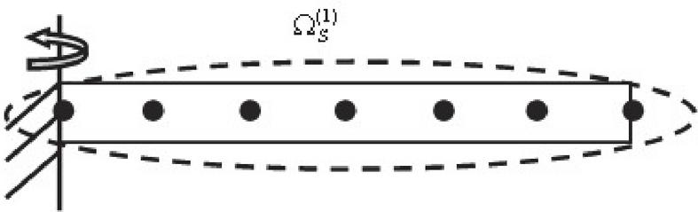
Figure 1 Nodal distribution on the rotating uniform beam.

The Gaussian radial basis functions are given by [1]

$$R_j(x)=e^{-c\frac{{(|x-x_j|)}^2}{s_j^2}}$$

(28)

The multiquadrics basis functions are given by [1]

$$R_j(x)={[{(|x-x_j|)}^2+{({\alpha }_c{d}_c)}^2]}^q$$

(29)

If ${\alpha }_c=1,d_c=1$ and $q=1$, we get the radial basis function which is given by

$$R_j(x)=[1+{(|x-x_j|)}^2]$$

(30)

Further we refine the Equation (30) as

$$R_j(x)=[1+|x-x_j|+{(|x-x_j|)}^2+{(|x-x_j|)}^3]$$

(31)

The Equation (31) is similar to conventional cubic approximation in finite element method. To get the new basis function (refined basis function) we multiply the right hand sides of Equations (28) and (31), which is given by Equation (32)

$$R_j(x)=[1+|x-x_j|+{(|x-x_j|)}^2+{(|x-x_j|)}^3]e^{-c\frac{{(|x-x_j|)}^2}{s_j^2}}$$

(32)

Equation (32) is the new basis function which provides better results for fourth and fifth natural frequencies. The results are more accurate for higher natural frequencies.

The transverse displacement can be written as

$\overline{w}(x)$	$=R_1(x)a_1+S_1(x)b_1+R_2(x)a_2+S_2(x)b_2$
	$\mathrm{\hspace{1em}}+\mathrm{\cdots }+R_N(x)a_N+S_N(x)b_N$	(33)

where, $N$ is the number of nodes, and $a_1,b_1,a_2,b_2,\mathrm{\dots },a_N,b_N$ are arbitrary constants. The derivative of the new basis function is given by

$$S_j(x)=\frac{d{R}_j(x)}{dx}$$

(34)

Here, values of $c$ and $s_j$ are user defined. The slope can be given by

$\theta (x)$	$={\displaystyle \frac{d{R}_1(x)}{dx}}{a}_1+{\displaystyle \frac{d{S}_1(x)}{dx}}{b}_1+{\displaystyle \frac{d{R}_2(x)}{dx}}{a}_2+{\displaystyle \frac{d{S}_2(x)}{dx}}{b}_2$
	$\mathrm{\hspace{1em}}+\mathrm{\cdots }+{\displaystyle \frac{d{R}_N(x)}{dx}}{a}_N+{\displaystyle \frac{d{S}_N(x)}{dx}}{b}_N$	(35)

The transverse displacement is given by

$$\overline{w}(x)={[Q(x)]}_{(1,2N)}{[c]}_{(2N,1)}^T$$

(36)

Here,

$${[Q(x)]}_{(1,2N)}=[R_1(x)S_1(x)R_2(x)S_2(x)\mathrm{\dots }{R}_N(x)S_N(x)]$$

(37)

and

$${[c]}_{(1,2N)}=[a_1{b}_1{a}_2{b}_2\mathrm{\dots }{a}_N{b}_N]$$

(38)

The slope is given by

$$\theta (x)={\left[\frac{dQ(x)}{dx}\right]}_{(1,2N)}{[c]}_{(2N,1)}^T$$

(39)

Here,

${\left[{\displaystyle \frac{dQ(x)}{dx}}\right]}_{(1,2N)}=\left[{\displaystyle \frac{d{R}_1(x)}{dx}}{\displaystyle \frac{d{S}_1(x)}{dx}}{\displaystyle \frac{d{R}_2(x)}{dx}}{\displaystyle \frac{d{S}_2(x)}{dx}}\mathrm{\dots }{\displaystyle \frac{d{R}_N(x)}{dx}}{\displaystyle \frac{d{S}_N(x)}{dx}}\right]$

(40)

After substituting the values of nodal points in Equations (36) and (39) we get

$${[Q_M]}_{(2N,2N)}{[c]}_{(2N,1)}^T={[d]}_{(2N,1)}$$

(41)

Here,

$${[d]}_{(1,2N)}=[w_1{\theta }_1{w}_2{\theta }_2\mathrm{\dots }{w}_N{\theta }_N]$$

(42)

and

$$[{\mathrm{Q}}_{\mathrm{M}}]=\left[\begin{array}{ccccccc}\hfill {\mathrm{R}}_1({\mathrm{x}}_1)\hfill & \hfill {\mathrm{S}}_1({\mathrm{x}}_1)\hfill & \hfill {\mathrm{R}}_2({\mathrm{x}}_1)\hfill & \hfill {\mathrm{S}}_2({\mathrm{x}}_1)\hfill & \hfill \mathrm{\cdots }\hfill & \hfill {\mathrm{R}}_{\mathrm{N}}({\mathrm{x}}_1)\hfill & \hfill {\mathrm{S}}_{\mathrm{N}}({\mathrm{x}}_1)\hfill \\ \hfill \frac{{\mathrm{dR}}_1({\mathrm{x}}_1)}{\mathrm{dx}}\hfill & \hfill \frac{{\mathrm{dS}}_1({\mathrm{x}}_1)}{\mathrm{dx}}\hfill & \hfill \frac{{\mathrm{dR}}_2({\mathrm{x}}_1)}{\mathrm{dx}}\hfill & \hfill \frac{{\mathrm{dS}}_2({\mathrm{x}}_1)}{\mathrm{dx}}\hfill & \hfill \mathrm{\cdots }\hfill & \hfill \frac{{\mathrm{dR}}_{\mathrm{N}}({\mathrm{x}}_{1)}}{\mathrm{dx}}\hfill & \hfill \frac{{\mathrm{dS}}_{\mathrm{N}}({\mathrm{x}}_1)}{\mathrm{dx}}\hfill \\ \hfill {\mathrm{R}}_1({\mathrm{x}}_2)\hfill & \hfill {\mathrm{S}}_1({\mathrm{x}}_2)\hfill & \hfill {\mathrm{R}}_2({\mathrm{x}}_2)\hfill & \hfill {\mathrm{S}}_2({\mathrm{x}}_2)\hfill & \hfill \mathrm{\cdots }\hfill & \hfill {\mathrm{R}}_{\mathrm{N}}({\mathrm{x}}_2)\hfill & \hfill {\mathrm{S}}_{\mathrm{N}}({\mathrm{x}}_2)\hfill \\ \hfill \frac{{\mathrm{dR}}_1({\mathrm{x}}_2)}{\mathrm{dx}}\hfill & \hfill \frac{{\mathrm{dS}}_1({\mathrm{x}}_2)}{\mathrm{dx}}\hfill & \hfill \frac{{\mathrm{dR}}_2({\mathrm{x}}_2)}{\mathrm{dx}}\hfill & \hfill \frac{{\mathrm{dS}}_2({\mathrm{x}}_2)}{\mathrm{dx}}\hfill & \hfill \mathrm{\cdots }\hfill & \hfill \frac{{\mathrm{dR}}_{\mathrm{N}}({\mathrm{x}}_2)}{\mathrm{dx}}\hfill & \hfill \frac{{\mathrm{dS}}_{\mathrm{N}}({\mathrm{x}}_2)}{\mathrm{dx}}\hfill \\ \hfill .\hfill & \hfill .\hfill & \hfill .\hfill & \hfill .\hfill & \hfill \mathrm{\cdots }\hfill & \hfill .\hfill & \hfill .\hfill \\ \hfill .\hfill & \hfill .\hfill & \hfill .\hfill & \hfill .\hfill & \hfill \mathrm{\cdots }\hfill & \hfill .\hfill & \hfill .\hfill \\ \hfill .\hfill & \hfill .\hfill & \hfill .\hfill & \hfill .\hfill & \hfill \mathrm{\cdots }\hfill & \hfill .\hfill & \hfill .\hfill \\ \hfill {\mathrm{R}}_1({\mathrm{x}}_{\mathrm{N}})\hfill & \hfill {\mathrm{S}}_1({\mathrm{x}}_{\mathrm{N}})\hfill & \hfill {\mathrm{R}}_2({\mathrm{x}}_{\mathrm{N}})\hfill & \hfill {\mathrm{S}}_2({\mathrm{x}}_{\mathrm{N}})\hfill & \hfill \mathrm{\cdots }\hfill & \hfill {\mathrm{R}}_{\mathrm{N}}({\mathrm{x}}_{\mathrm{N}})\hfill & \hfill {\mathrm{S}}_{\mathrm{N}}({\mathrm{x}}_{\mathrm{N}})\hfill \\ \hfill \frac{{\mathrm{dR}}_1({\mathrm{x}}_{\mathrm{N}})}{\mathrm{dx}}\hfill & \hfill \frac{{\mathrm{dS}}_1({\mathrm{x}}_{\mathrm{N}})}{\mathrm{dx}}\hfill & \hfill \frac{{\mathrm{dR}}_2({\mathrm{x}}_{\mathrm{N}})}{\mathrm{dx}}\hfill & \hfill \frac{{\mathrm{dS}}_2({\mathrm{x}}_{\mathrm{N}})}{\mathrm{dx}}\hfill & \hfill \mathrm{\cdots }\hfill & \hfill \frac{{\mathrm{dR}}_{\mathrm{N}}({\mathrm{x}}_{\mathrm{N}})}{\mathrm{dx}}\hfill & \hfill \frac{{\mathrm{dS}}_{\mathrm{N}}({\mathrm{x}}_{\mathrm{N}})}{\mathrm{dx}}\hfill \end{array}\right].$$

(43)

Here, $w_1,{\theta }_1,w_2,{\theta }_2,\mathrm{\dots },w_N,{\theta }_N$ are the nodal degrees of freedom.

We can write Equation (41) as

$${[c]}_{(2N,1)}^T={[Q_M]}_{(2N,2N)}^{-1}{[d]}_{(2N,1)}$$

(44)

From Equations (36) and (41), we get

$$\overline{w}(x)={[H(x)]}_{(1,2N)}{[d]}_{(2N,1)}$$

(45)

where, $[H(x)]$ is the shape function vector.

${[H(x)]}_{(1,2N)}$	$={[Q(x)]}_{(1,2N)}{[Q_M]}_{(2N,2N)}^{-1}$
	$=[{\varphi }_1^{(w)}(x)\mathit{\hspace{1em}}{\varphi }_1^{(\theta )}(x)\mathit{\hspace{1em}}{\varphi }_2^{(w)}(x)\mathit{\hspace{1em}}{\varphi }_2^{(\theta )}(x){\varphi }_N^{(w)}(x){\varphi }_N^{(\theta )}(x)]$	(46)

Here, ${\varphi }_i^{(w)}(x)$ and ${\varphi }_i^{(\theta )}(x)$ are the shape functions related with node $i$.

The transverse displacement is given by

$$\overline{w}(x)=\sum _{j=1}^N({\varphi }_j^{(w)}(x)w_j+{\varphi }_j^{(\theta )}(x){\theta }_j)$$

(47)

In Galerkin method, the test function is given by

$$v(x)=\sum _{j=1}^N({\varphi }_j^{(w)}(x)\delta w_j+{\varphi }_j^{(\theta )}(x)\delta {\theta }_j)$$

(48)

The meshfree stiffness and mass matrices are given by

${[K]}_{{\mathrm{\Omega }}_S^{(i)}}$	$={\displaystyle {\int }_{{\mathrm{\Omega }}_S^{(i)}}}g(\zeta ){\displaystyle \frac{d^2{[H]}^T}{d{\zeta }^2}}{\displaystyle \frac{d^2[H]}{d{\zeta }^2}}\mathit{d}\zeta +{\displaystyle {\int }_{{\mathrm{\Omega }}_S^{(i)}}}{s}^{2}h(\zeta ){\displaystyle \frac{d{[H]}^T}{d\zeta }}{\displaystyle \frac{d[H]}{d\zeta }}\mathit{d}\zeta$
	$\mathrm{\hspace{1em}\hspace{1em}}-{\displaystyle {\int }_{{\mathrm{\Omega }}_S^{(i)}}}{\displaystyle \frac{s^2}{r^2}}g(\zeta ){\displaystyle \frac{d{[H]}^T}{d\zeta }}{\displaystyle \frac{d[H]}{d\zeta }}\mathit{d}\zeta$	(49)
${[M]}_{{\mathrm{\Omega }}_S^{(i)}}$	$={\displaystyle {\int }_{{\mathrm{\Omega }}_S^{(i)}}}f(\zeta ){[H]}^T[H]\mathit{d}\zeta +{\displaystyle {\int }_{{\mathrm{\Omega }}_S^{(i)}}}{\displaystyle \frac{1}{r^2}}g(\zeta ){\displaystyle \frac{d{[H]}^T}{d\zeta }}{\displaystyle \frac{d[H]}{d\zeta }}\mathit{d}\zeta$	(50)

To explain the meshfree Galerkin method, we have number of subdomains shown in Figure 2. The algebraic equations can be written for each element and assembled where the essential boundary conditions are applied.

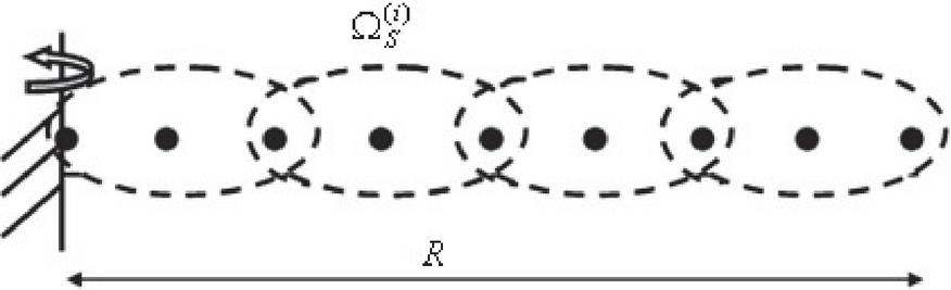
Figure 2 Nodal distribution and local support domains for the meshfree finite element method.

Figure 3 shows the plots for shape function and shape function derivative.

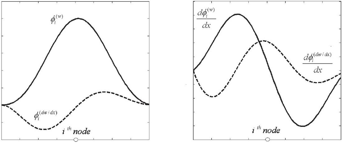
Figure 3 (a) and (b): Variations of the shape function and the shape function’s derivative, respectively.

5 Results and Discussion

The results are obtained for the rotating and non-rotating Rayleigh beam. The results discuss both Gaussian radial basis function and refined radial basis functions. Also, the results are obtained for the rotating Euler-Bernoulli beams for comparison. Here, we consider only six nodes within the subdomain. The results are obtained for varying non-dimensional parameters $r$ and $s$ which are explained in Section 3. Here, Tables 1 and 3 show the result of a non-rotating beam and in Tables 2 and 4 show the result of rotating beams. For each Table corresponding mode shapes are shown in Figures. The results of conventional finite element have been obtained where forty elements are considered within the domain. In Figures 8(a) and 8(b), the results are compared for both the beams.

Table 1 Non-dimensional natural frequencies of a non-rotating Rayleigh beam

$r=10,s=0,\overline{n}=1,c=1/2$					$r=100,s=0,\overline{n}=1,c=1/2$
			Gaussian	Refined			Gaussian	Refined
			Radial	Radial			Radial	Radial	FEM
		FEM	Basis	Basis		FEM	Basis	Basis	$(n=40)$
	[25]	$n=40$	Function	Function	[25]	$n=40$	Function	Function	(E-B)
${\lambda }_1$	3.7727	3.7727	3.7727	3.7727	3.8233	3.8233	3.8233	3.8233	3.8238
${\lambda }_2$	17.097	17.0975	17.0975	17.0975	18.304	18.3038	18.3038	18.3038	18.3173
${\lambda }_3$	40.412	40.4126	40.4125	40.4125	47.178	47.1781	47.1780	47.1780	47.2649
${\lambda }_4$	N/A	69.4402	69.4395	69.4401	N/A	90.1371	90.1351	90.1356	90.4509
${\lambda }_5$	N/A	101.4261	101.4587	101.4447	N/A	147.1728	147.3387	147.3258	148.0035

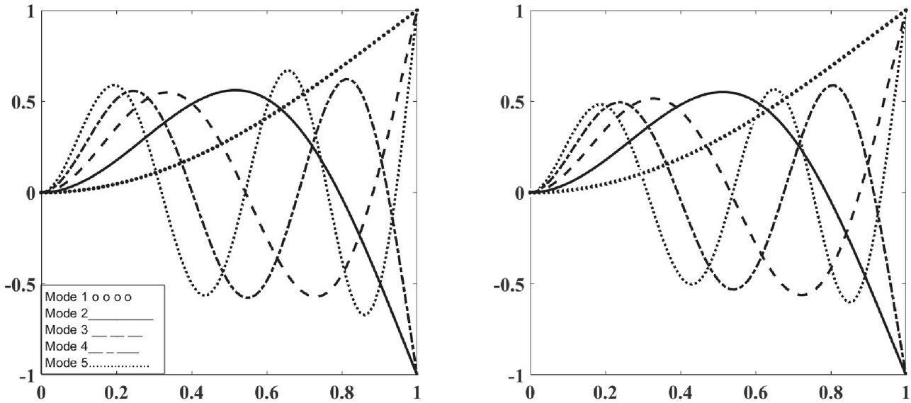
Figure 4 (a) and (b): Mode shapes of a non-rotating beam for $r=10,s=0,\overline{n}=1,c=1/2$ and $r=100,s=0,\overline{n}=1,c=1/2$.

Table 2 Non-dimensional natural frequencies of a rotating Rayleigh beam

$r=10,s=5,\overline{n}=1,c=1/2$					$r=100,s=5,\overline{n}=1,c=1/2$
			Gaussian	Refined			Gaussian	Refined
			Radial	Radial			Radial	Radial	FEM
		FEM	Basis	Basis		FEM	Basis	Basis	$(n=40)$
	[25]	$n=40$	Function	Function	[25]	$n=40$	Function	Function	(E-B)
${\lambda }_1$	6.6118	6.6118	6.6118	6.6118	6.7421	6.7421	6.7421	6.7421	6.7434
${\lambda }_2$	20.356	20.3563	20.3563	20.3563	21.888	21.8883	21.8882	21.8882	21.9053
${\lambda }_3$	43.444	43.4436	43.4436	43.4436	50.839	50.8391	50.8390	50.8390	50.9339
${\lambda }_4$	N/A	72.2411	72.2403	72.2407	N/A	93.8788	93.8762	93.8764	94.2067
${\lambda }_5$	N/A	103.9772	104.0090	103.9972	N/A	150.9629	151.1378	151.1284	151.8160

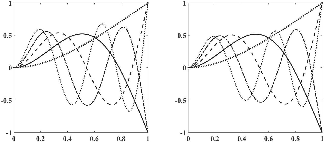
Figure 5 (a) and (b): Mode shapes of a non-rotating beam for $r=10,s=5,\overline{n}=1,c=1/2$ and $r=100,s=5,\overline{n}=1,c=1/2$.

Table 3 Non-dimensional natural frequencies of a non-rotating Rayleigh beam

$r=10,s=0,\overline{n}=2,c=1/2$					$r=100,s=0,\overline{n}=2,c=1/2$
			Gaussian	Refined			Gaussian	Refined
			Radial	Radial			Radial	Radial	FEM
		FEM	Basis	Basis		FEM	Basis	Basis	$(n=40)$
	[25]	$n=40$	Function	Function	[25]	$n=40$	Function	Function	(E-B)
${\lambda }_1$	4.5517	4.5517	4.5517	4.5517	4.6244	4.6244	4.6244	4.6244	4.6251
${\lambda }_2$	18.211	18.2107	18.2107	18.2107	19.533	19.5328	19.5328	19.5328	19.5476
${\lambda }_3$	41.457	41.4573	41.4572	41.4572	48.489	48.4886	48.4885	48.4885	48.5790
${\lambda }_4$	N/A	70.3744	70.3737	70.3746	N/A	91.4925	91.4906	91.4912	91.8132
${\lambda }_5$	N/A	102.2365	102.2407	102.2271	N/A	148.5498	148.6896	148.6769	149.3917

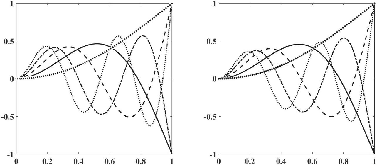
Figure 6 (a) and (b): Mode shapes of a non-rotating beam for $r=10,s=0,\overline{n}=2,c=1/2$ and $r=100,s=0,\overline{n}=2,c=1/2.$

Table 4 Non-dimensional natural frequencies of a rotating Rayleigh beam

$r=10,s=5,\overline{n}=2,c=1/2$					$r=100,s=5,\overline{n}=2,c=1/2$
			Gaussian	Refined			Gaussian	Refined
			Radial	Radial			Radial	Radial	FEM
		FEM	Basis	Basis		FEM	Basis	Basis	$(n=40)$
	[25]	$n=40$	Function	Function	[25]	$n=40$	Function	Function	(E-B)
${\lambda }_1$	7.1268	7.1268	7.1268	7.1268	7.2885	7.2885	7.2885	7.2885	7.2901
${\lambda }_2$	21.003	21.0033	21.0033	21.0033	22.618	22.6179	22.6179	22.6179	22.6360
${\lambda }_3$	44.014	44.0143	44.0143	44.0143	51.595	51.5945	51.5945	51.5945	51.6919
${\lambda }_4$	N/A	72.7026	72.7018	72.7023	N/A	94.6302	94.6276	94.6278	94.9630
${\lambda }_5$	N/A	104.3394	104.3527	104.3406	N/A	151.7073	151.8609	151.8509	152.5683

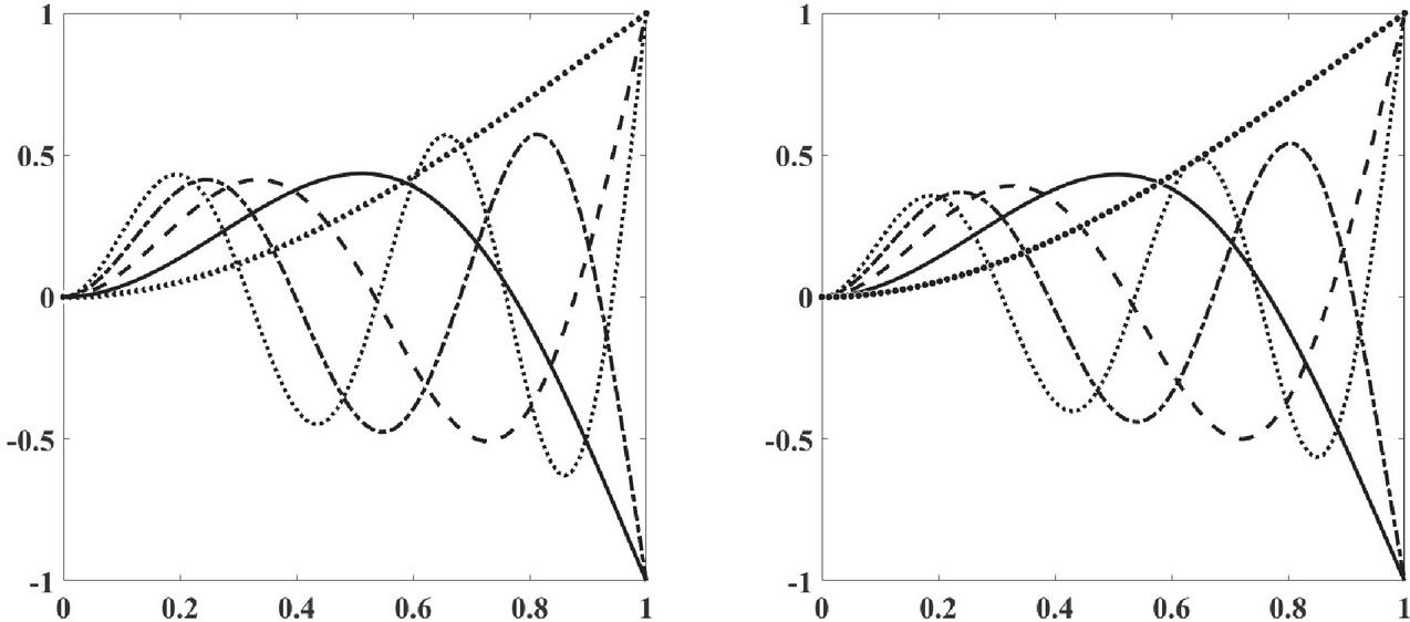
Figure 7 (a) and (b): Mode shapes of a non-rotating beam for $r=10,s=5,\overline{n}=2,c=1/2$ and $r=100,s=5,\overline{n}=2,c=1/2.$

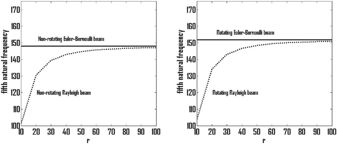
Figure 8 (a) and (b): Variation in the fifth natural frequency with change in the slenderness ratio for a non-rotating and a rotating beam, respectively.

6 Conclusions

In this paper, the rotating and non-rotating Rayleigh beam problems have been using the meshfree Galerkin method where new radial basis functions (refined radial basis functions) are developed and results are found more accurate than the Gaussian radial basis functions for the third and fourth natural frequencies when only six nodes are considered within the subdomain of trial and test function. Both multiquadrics radial basis functions and Gaussian radial basis functions are multiplied to get the new basis function. Also, the results of rotating Euler-Bernoulli obtained to have a comparison of change in natural frequency. For conventional finite element method forty elements are considered within the domain. Stiffness and mass matrices have been derived for in non-dimensional form as well. The results are found accurate when compared to literature and conventional finite element method.

References

[1] G. R. Liu, Y. T. Gu, An Introduction to Meshfree Methods and Their Programming, Springer, New York, 2005.

[2] I. S. Raju, D. R. Phillips, T. Krishnamurthy, A radial basis function approach in the meshless local Petrov-Galerkin method for Euler-Bernoulli beam problems, Computational Mechanics, 34, 464–474, 2004.

[3] Y. Duan, Y.-J. Tan, A meshless Galerkin method for Dirichlet problems using radial basis functions, Journal of Computational and Applied Mathematics, 196, 394–401, 2006.

[4] H. Wendland, Meshless Galerkin methods using radial basis functions, Mathematics of Computation, 68, 1521–1531, 1999.

[5] S-u-Islam, B. Sarler, R. Vertnik, G. Kosec, Radial basis function collocation method for the numerical solution of the two-dimensional transient nonlinear coupled Burgers’ equations, Applied Mathematical Modelling, 36, 1148–1160, 2012.

[6] T. Huang, Q. X. Pan, J. Jin, J. L. Zheng, P. H. Wen, Continuous constitutive model for bimodulus materials with meshless approach, Applied Mathematical Modelling, 66, 41–58, 2019.

[7] K. Zhu, J. Chung, Vibration and stability analysis of a simply-supported Rayleigh beam with spinning and axial motions, Applied Mathematical Modelling, 66, 362–382, 2019.

[8] H. D. Hodges, M. J. Rutkowski, Free-vibration analysis of rotating beams by a variable-order finite element method, AIAA Journal, 19, 1459–1466, (1981).

[9] V. T. Nagaraj, P. Shanthakumar, Rotor blade vibration by the Galerkin finite element method, Journal of Sound and Vibration, 43, 575–577, 1975.

[10] O. A. Bauchau, C. H. Hong, Finite element approach to rotor blade modeling, Journal of the American Helicopter Society, 32, 60–67, 1987.

[11] S. V. Hoa, Vibration of a rotating beam with tip mass, Journal of Sound and Vibration, 67, 369–381, 1979.

[12] J. B. Gunda, R. Ganguli, Stiff-string basis functions for vibration analysis of high speed rotating beams, Journal of Applied Mechanics, 75, 0245021–25, 2007.

[13] J. B. Gunda, R. K. Gupta, R. Ganguli, Hybrid stiff-string-polynomial basis functions for vibration analysis of high speed rotating beam, Computers and Structures, 87, 254–265, 2008.

[14] D. Sushma, R. Ganguli, A collocation approach for finite element basis functions for Euler-Bernoulli beams undergoing rotations and transverse bending vibration, International Journal for Computational Methods in Engineering Science and Mechanics, 13, 290–307, 2012.

[15] V. Panchore, R. Ganguli, S. N. Omkar, Meshless local Petrov-Galerkin method for rotating Euler-Bernoulli beam, Computer Modeling in Engineering and Sciences, 104, 353–373, 2015.

[16] V. Panchore, R. Ganguli, S. N. Omkar, Meshless local Petrov-Galerkin method for rotating Timoshenko beam: A locking-free shape function formulation, Computer Modeling in Engineering and Sciences, 108, 215–237, 2015.

[17] V. Panchore, R. Ganguli, Quadratic B-spline finite element method for a rotating non-uniform Rayleigh beam, Structural Engineering Mechanics, 61, 765–773, 2017.

[18] D. Adair, M. Jaeger, Simulation of tapered rotating beams with centrifugal stiffening using the Adomian decomposition method, Applied Mathematical Modelling, 40, 3230–3241, 2016.

[19] K. G. Vinod, S. Gopalakrishnan, R. Ganguli, Free vibration and wave propagation analysis of uniform and tapered rotating beams using spectrally formulated finite elements, International Journal of Solids and Structures, 44, 5875–5893, 2007.

[20] V. Giurgiutiu, R. O. Stafford, Semi-analytical methods for frequencies and mode shapes of rotor blades, Vertica, 1, 291–306, 1977.

[21] Y. Chen, X. Guo, D. Zhang, L. Li, Dynamic modeling and analysis of rotating FG beams for capturing steady bending deformation, Applied Mathematical Modelling, 88, 498–517, 2020.

[22] R. Ganguli, V. Panchore, The rotating beam problem in helicopter dynamics, Springer, Singapore, 2018.

[23] R. Ganguli, Finite element analysis of rotating beams, Springer, Singapore, 2017.

[24] V. Panchore, R. Ganguli, S. N. Omkar, Meshfree Galerkin Method for a rotating Euler-Bernoulli beam, International Journal for Computational Methods in Engineering Science and Mechanics, 19, 11–21, 2017.

[25] J. R. Banerjee, D. R. Jackson, Free vibration of a rotating tapered Rayleigh beam: A dynamic stiffness method of solution, Computers and Structures, 124, 11–20, 2013.

Biography

Vijay Panchore received the bachelor’s degree in Industrial engineering from NIT Jalandhar in 2009, the master’s degree in Design engineering from IISc Bangalore in 2011, and the philosophy of doctorate degree in Aerospace Engineering from IISc Bangalore in 2017, respectively. He is currently working as an Assistant Professor at the Department of Mechanical Engineering, Maulana Azad National Institute of Technology, Bhopal, 462003, India.

European Journal of Computational Mechanics, Vol. 30_4–6, 501–518.
doi: 10.13052/ejcm2642-2085.30469
© 2022 River Publishers

Abstract

1 Introduction

2 Weak Formulation of the Governing Differential Equation

3 Rotating Rayleigh Beam Equation in Non-dimensional Form

4 Radial Basis Function Interpolation for Meshfree Method

5 Results and Discussion

6 Conclusions

References

Biography