Stress Analysis by Two Cuboid Isoparametric Elements

Mohammad Rezaiee-Pajand* and Arash Karimipour

Department of Civil Engineering, Ferdowsi University of Mashhad, Iran

Email: rezaiee@um.ac.ir

* Corresponding Author

Received 28 July 2019; Accepted 03 December 2019; Publication 18 December 2019

Abstract

The finite element method is a powerful tool for solving most of the structural problems. This technique has been used extensively, since the complexity of the elastic field equations does not allow the specialist to find analytical solutions, especially for the three-dimensional structures. It is well-known that the finite element formulation yields the approximate stress responses. To remedy this defect, the Airy stress function is utilized in this study. The stress function formulation leads to a valid solution since it satisfies equilibrium and compatibility equations simultaneously. Two cuboid isoparametric elements are formulated for solving three-dimensional elastic structures. To demonstrate the performance of the proposed technique, various benchmark problems are analyzed. The errors between the exact, displacement-based finite element and recommended scheme solution are also calculated. All the obtained outcomes show the good merit of the presented new elements.

Keywords: Finite element method, precise stress, analytical formulation, cuboid element, accurate displacement.

Notation

U	Interior of a closed curve G in the xy-plane
um	Displacement fields in the member
σxx	Vertical stress component in x-direction
ν	Poisson’s ratio
V	Scalar potential
fsim	Simulation values
f, g and h	Uniform functions defining position on G
ℒ	Set of linear differential operatives
σyy	Vertical stress component in the y-direction
φ	Shape function
MAPE	Mean absolute percentage error
σm	Stress fields in the member
σzz	Vertical stress component in z-direction
μ	Modulus of elasticity
r	Position vector
fana	Analytical values

Introduction

Finite element method has different elements to solve a great variety of problems. Displacement techniques are common ways to formulate a new element. The weakness of this scheme is mostly leading to inaccurate stresses. There are several ways to remedy this fault and improve the responses. In one of the studies, an 8-node element was selected, and the Airy function was utilized to establish a new element by Fu et al. in 2008 [1]. The performance of this element was carefully evaluated by the researchers, which showed some improvements. It should be reminded that the Airy stress function can give more accurate stress. This function is determined so that the prescribed boundary conditions at a far field and the continuity condition of the traction force, along with the displacement field at the interface are satisfied exactly.

In another study, Lee and Bathe studied some influences achieved by 8-node and 12-node and also Lagrangian (Q9, Q16) elements by using numerical analyses with different meshes [2]. Their obtained results showed that displacement outcomes of the 8-node element were more accurate than when 12-node was selected. In 1999, Kikuchi et al. modified the 8-node model by defining a new principle of 8-node spaces and using the Cartesian quadratic polynomial space. This principle was established when the quadrilateral had eight nodes. However, this element could not properly represent the behavior of the Cartesian quadratic polynomials in the fully isoperimetric cases [3]. Li et al. proposed a new 8-node element by paying attention to Kikuchi’s research. Their study led to the simpler formulations for this element [4].

In 2003, Rajendran and Liew used two different shape functions, namely metric set and isoperimetric set, as the trial and test functions, respectively [5]. In their study, the 8-node element was utilized based on unsymmetrical element stiffness matrix. Their formulations represented an excellent performance for this element. These findings highly fitted the results of several exact solutions. In 2006, Li and Wang proposed a new 8-node spline element. According to their study, accurate outcomes for several problems can be achieved by utilizing a relatively complicated mathematical treatment [6]. In another research, Long et al. established a new coordinate system. This was followed by developing 8-node element by Soh et al. [7] and Cen et al. [8], respectively.

There are other studies focusing on systematical discussions of this topic based on the finite element method [9]. The principle of minimum potential energy forms the basis of the method in all of these researches [10, 11]. In another study, a new formula was established for elasticity problems [12]. Although the error in this approach was obvious, this technique led to the direct and simple solution for determining the strain values. For this purpose, a formula was obtained by using poor performance of the current direct formulations, based on the strain and material property distribution. In 2012, Cervera et al. proposed an analytical solution for bifurcation, localization, stress bounded and the DE cohesion conditions for the elasticity problems [13]. This study showed that a mixed displacement-pressure formulation was suitable and provided accurate performance for predicting correct failure mechanisms with the localized patterns of plastic deformation in plasticity problems. Artioli et al. recognized a numerical solution for 2D elasticity problems. In their study, the theory of strain was considered along with mixed Hellinger–Reissner variational formulation. Recently, Rezaiee-Pajand and Karimipour presented three new triangular elements [14]. In their investigation, complementary energy functional, along with the Airy stress function, were utilized within an element for the analysis of plane problems. To validate the results, extensive numerical studies were accomplished. The findings clearly demonstrated the accuracies of structural displacements, as well as, stresses.

So far, the properties of the 8-node element and its improvement by stress function were revealed. According to the available literature, there have been some activities in utilizing the Airy function for solving structural problems. In Fosdick and Schuler research, a generalized Airy stress function was presented, which preserved smoothness and also completeness [15]. The generalized form identified the explicit additional pieces that were needed for completeness in the multiply connected domains. This study by Fosdick and Schuler was performed for the case when a body force field was presented. In another research, Zavelani-Ross established a finite element technique for plane stress problems [16]. To solve in-plane free vibration arch shape members, Nieh et al. presented an analytical solution in 2003 [17]. They considered the effect of the extensibility of the arch shape members and neglected the effect of shear deformation. In order to establish an analytical solution for the free vibration of arch members with varying curvature, a series solution was proposed. As a result, the suggested scheme played an accurate role in predicting arc behavior.

In another investigation, Serra proposed approximate analytical and numerical solutions [18]. In this study, the arch shape members were analyzed under the static loads, and two approximate solutions were utilized. Furthermore, the related code for the latter solution was given. In 1988, HarikGhassan and Salamoun defined an analytical strip method for solving the rectangular plates [19]. In their investigation, the plate was modelled as a system of plate strips and beam segments rigidly connected to each other. For this structure, the closed-form solution was derived. By avoiding the polynomial representation and minimization procedure, they took advantages of the semi-analytical finite strip method in the mentioned study. The obtained outcomes indicated that the stiffened and unstiffened rectangular plates with different edge and loading conditions could be solved exactly by their method.

In order to determine the shear behavior of plate elements, Karttunen et al. used an exact elasticity solution [20]. They presented a general exact 3-D plate solution. Their element had four nodes. In fact, the general plate solution was derived by a bi-harmonic mid-surface function. This function was appropriate for the thick plate elements. Furthermore, the 3-D Navier equations of elasticity and the Kirchhoff constraints were used for the development of the finite element model. In 1989, Arya presented an analytical and finite element solution for some problems by using a viscoplastic model [21]. This researcher performed a nonlinear structural analysis. The proposed scheme could analyze thick-walled cylinder, thin rotating disk and thick-walled sphere. The analytical expressions derived for the stress and the strain rates for these components were general in nature. Moreover, they considered both the time-depended mechanical and thermal loadings. The achieved consequences showed that the possibility of the viscoplastic model could play an appropriate role in the nonlinear structural analyses.

Zhang et al. presented a Three-dimensional damage analysis by using FEM [22]. They proposed the damage of members in three-dimensional space. In order to reduce the number of degrees of freedoms, an automatic mesh generation algorithm was employed. To illustrate the mesh-independence, a double-notched tension beam was simulated with two different meshes. According to the obtained outcomes, the projected computational method was adept of accurately catching the damage progress under complicated boundary conditions. Shang et al. used FEM for solving Euler-Bernoulli beam problems [23]. They presented a dynamic analysis scheme. By this technique, analysis of a bar was achieved by using several enhancement stages. In this process, error measures and nonlinear strains were projected. The obtained results demonstrated that the presented scheme had good accuracy. In 2018, two-dimensional orthotropic elasticity problems were solved by the help of Airy stress function [24]. A simple 8-node element with 16-DOF was utilized in this procedure. All numerical tests demonstrated that this quadratic element could reach the exact solutions in constant and linear stress cases. In 2016, a new technique was utilized to solve boundary value problems [25]. Unlike the displacement technique, these problems were solved by the help of implicit function, which relates linearized strain and stress. These investigators assumed that the stress and the displacement were unknowns. Then, both the equilibrium equations and continuity of displacements were enforced precisely. The mentioned actions led to estimate the unknowns of the stress and displacement and created an efficient scheme.

Based on the available literature, some plane elements have been presented by using Airy stress functions, so far. To solve the three-dimensional problems, solid elements, based on the assumed displacement, are mostly utilized. To the best knowledge of the authors, no hybrid three-dimensional rectangular element has been proposed up to this date, which has utilized the Airy stress functions. Since this kind of elements is very useful in the use of irregular meshes, two new three-dimensional hybrid rectangular elements are presented in this article. Both suggested elements are isoparametric types. All formulations utilize Airy stress functions. Comprehensive studies are performed to calculate and validate the obtained displacement and stress. All findings clearly demonstrate very good accuracies.

Research Significance

The presented method employs the Airy stress function. This scheme reduces the general formulation to a single governing equation in terms of a single unknown. In this article, the mentioned governing equation is utilized by the finite element technique. Since the stress function formulation satisfies both equilibrium and compatibility conditions, it can lead to good responses for displacement as well as stress. According to the literature review, many studies have been done for increasing the response accuracy of the plane structures. Airy-stress function is one of the useful schemes, which leads to the suitable outcomes with good accuracy and low computation time. So far, no three-dimensional elements, based on the Airy stress function have been suggested. This study aims to perform some stress analyses by two new cuboid isoparametric elements. Solved problems will demonstrate that the authors’ elements are able to analyze three-dimensional elasticity problems efficiently.

Energy Functional for Airy Stress Function

Energy methods are a useful tool to solve different problems. These schemes are based on complementary energy formulas. In the finite element method, the complementary energy functional can be written in the next form:

$${\Pi }_C={\Pi }_C^{*}+V_C^{*}=\frac{1}{2}{\displaystyle \int {\displaystyle \int {\displaystyle {\int }_{V^e}^1{\sigma }^{T}C\sigma \mathit{dV}-}}}{\displaystyle {\int }_{\Gamma }^1{T}^T\overline{U}\mathit{ds}}$$

(1)

This equation has the following parts:

$$\sigma =\left\{\begin{array}{c}{\sigma }_x\\ {\sigma }_y\\ {\sigma }_z\\ {\tau }_{xy}\\ {\tau }_{xz}\\ {\tau }_{yz}\end{array}\right\}$$

(2)

$$\begin{array}{l}C=\frac{E}{(1+\mu )(1-2\mu )}\hfill \\ \times \left[\begin{array}{cccccc}1-\mu & \mu & \mu & 0& 0& 0\\ \mu & 1-\mu & \mu & 0& 0& 0\\ \mu & \mu & 1-\mu & 0& 0& 0\\ 0& 0& 0& \frac{1-2\mu }{2}& 2& 0\\ 0& 0& 0& 0& \frac{1-2\mu }{2}& 2\\ 0& 0& 0& 0& 0& \frac{1-2\mu }{2}\end{array}\right]\hfill \end{array}$$

(3)

$$T=\left\{\begin{array}{c}{T}_x\\ T_y\\ T_z\end{array}\right\}$$

(4)

$$\overline{U}=\left\{\begin{array}{c}\overline{u}\\ \overline{v}\\ \overline{w}\end{array}\right\}$$

(5)

Where, ${\Pi }_C^{*}$ and $V_C^{*}$ are the complementary energy within the element and along the element boundaries, respectively. Furthermore, σ is the stress vector, T is the surface traction force vector through the element boundaries, U is the displacement vector along the element boundaries, and C is the elastic flexibility matrix. It should be mentioned that Young’s modulus (E) and Poisson’s ratio (μ) in all directions are constant. The relation between the Airy stress function, φ, and the stress vector, σ, is as follows:

$$\sigma =\left\{\begin{array}{c}{\sigma }_x\\ {\sigma }_y\\ {\sigma }_z\\ {\tau }_{xy}\\ {\tau }_{xz}\\ {\tau }_{zy}\end{array}\right\}=\left\{\begin{array}{r}\hfill \frac{{\partial }^2\phi }{\partial y^2}\\ \hfill \frac{{\partial }^2\phi }{\partial x^2}\\ \hfill \frac{{\partial }^2\phi }{\partial z^2}\\ \hfill -\frac{{\partial }^2\phi }{\partial x\partial y}\\ \hfill -\frac{{\partial }^2\phi }{\partial x\partial z}\\ \hfill -\frac{{\partial }^2\phi }{\partial z\partial y}\end{array}\right\}=\tilde{R}(\phi )$$

(6)

Utilizing the direction cosines, the surface force vector can be written by:

$$T=\left\{\begin{array}{c}{T}_x\\ T_y\\ T_z\end{array}\right\}=\left[\begin{array}{llllll}l\hfill & 0\hfill & 0\hfill & m\hfill & m\hfill & 0\hfill \\ 0\hfill & m\hfill & 0\hfill & l\hfill & 0\hfill & l\hfill \\ 0\hfill & 0\hfill & n\hfill & 0\hfill & n\hfill & n\hfill \end{array}\right]\left\{\begin{array}{c}{\sigma }_x\\ {\sigma }_y\\ {\sigma }_z\\ {\tau }_{xy}\\ {\tau }_{xz}\\ {\tau }_{zy}\end{array}\right\}=L\tilde{R}\left(\phi \right)$$

(7)

$$L=\left[\begin{array}{cccccc}l& 0& 0& m& m& 0\\ 0& m& 0& l& 0& l\\ 0& 0& n& 0& n& n\end{array}\right]$$

(8)

Where l, m and n are the direction cosines of the outer normal n in the element boundaries. By substituting equations (6) and (7) into (1), the complementary energy functional can be written in the next form:

$${\Pi }_C={\Pi }_C^{*}+V_C^{*}=\frac{1}{2}{\displaystyle \int {\displaystyle \int {\displaystyle {\int }_{V^e}^1\tilde{R}{(\phi )}^{T}C\tilde{R}(\phi )\mathit{dV}}}}-{\displaystyle {\int }_{\Gamma }^1{(L\tilde{R}\left(\phi \right))}^T\overline{U}\mathit{ds}}$$

(9)

So far, based on the basic relationships of the finite element method, the element complementary energy functional containing the Airy stress function is established.

Analytical Solutions by Stress Function

In the three-dimensional problems, without body forces, the Airy stress satisfies the following equation:

$${\nabla }^6\phi =\frac{{\partial }^6\phi }{\partial y^6}+3\frac{{\partial }^6\phi }{\partial x^3\partial y^3}+\frac{{\partial }^6\phi }{\partial x^6}+3\frac{{\partial }^6\phi }{\partial x^3\partial z^3}+\frac{{\partial }^6\phi }{\partial z^6}+3\frac{{\partial }^6\phi }{\partial y^3\partial z^3}$$

(10)

In order to choose appropriate trial functions for establishing a new element model, the next principles should be taken into account:

• (1) The basic analytical solutions of the stress function should be selected, which include the terms from the lowest-order to the higher-order.
• (2) The resulting stress fields should possess completeness in the Cartesian Coordinates.

In this study, two new 3D elements are formulated. One of them is an eight-node rectangular prism or cuboid element, which is named A3D8. As it is demonstrated in Figure 1, this element possesses eight nodes and twenty-four degrees of freedom. The second suggested element, which is called A3D20, has twenty nodes and sixty degrees of freedom. According to Figure 1, all the nodes are located in the element sides and corners. These types of elements are suggested to reach appropriate displacement, as well as, stress outputs. Their convergence powers to the exact solutions are also studied. According to the number of nodes and degrees of freedom in the element, stress function can be determined.

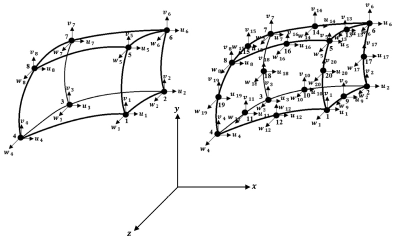
Figure 1 Tow proposed cuboid elements, A3D8 and A3D20.

Calculating the Interpolation Functions

At this stage, the degrees of freedom for the new elements are defined. As it is presented in Figure 1, the element nodal displacement vector, q^e, for A3D8 has the next form:

$$q_8^e=\left[\begin{array}{ccccccccccccc}{u}_1& v_1& w_1& u_2& v_2& w_2& u_3& v_3& w_3& u_4& v_4& w_4& u_5\\ v_5& w_5& u_6& v_6& w_6& u_7& v_7& w_7& u_8& v_8& w_8& & \end{array}\right]$$

(11)

A3D20 has the following degrees of freedom:

$$q_{12}^e=\left[\begin{array}{ccccccccccc}{u}_1& v_1& w_1& u_2& v_2& w_2& u_3& v_3& w_3& u_4& v_4\\ w_4& u_5& v_5& w_5& u_6& v_6& w_6& u_7& v_7& w_7& u_8\\ v_8& w_8& u_9& v_9& w_9& u_{10}& v_{10}& w_{10}& u_{11}& v_{11}& w_{11}\\ u_{12}& v_{12}& w_{12}& u_{13}& v_{13}& w_{13}& u_{14}& v_{14}& w_{14}& u_{15}& v_{15}\\ w_{15}& u_{16}& v_{16}& w_{16}& u_{17}& v_{17}& w_{17}& u_{18}& v_{18}& w_{18}& u_{19}\\ v_{19}& w_{19}& u_{20}& v_{20}& w_{20}& & & & & & \end{array}\right]$$

(12)

Where, u_i, v_i and w_i are the nodal displacements belonged to the x, y and z directions, respectively. Based on these degrees of freedom, there are different analytical solutions for the stress function. All of them are presented in Tables 1 and 2. Both suggested elements are isoparametric types. In the subsequent lines, the interpolation functions are found. For A3D8, the next relationships are calculated and verified:

$$N_8=\left\{\begin{array}{c}{N}_1\\ N_2\\ N_3\\ N_4\\ N_5\\ N_6\\ N_7\\ N_8\end{array}\right\}=\left\{\begin{array}{c}\frac{1}{8}(1-\xi )(1-\eta )(1-\zeta )\\ \frac{1}{8}(1+\xi )(1-\eta )(1-\zeta )\\ \frac{1}{8}(1+\xi )(1+\eta )(1-\zeta )\\ \frac{1}{8}(1-\xi )(1+\eta )(1-\zeta )\\ \frac{1}{8}(1-\xi )(1-\eta )(1+\zeta )\\ \frac{1}{8}(1+\xi )(1-\eta )(1+\zeta )\\ \frac{1}{8}(1+\xi )(1+\eta )(1+\zeta )\\ \frac{1}{8}(1-\xi )(1+\eta )(1+\zeta )\end{array}\right\}$$

(13)

Table 1 Basic analytical solutions of stress function and stresses for plane problem using A3D8

	i	1	2	3	4	5	6	7	8	9	10	11	12
	φi	x2	xy	y2	yz	z2	x2z	x3	x2y	y2x	z2x	y3	x2z
	σx	0	0	2	0	0	0	0	0	2x	0	6y	0
	σy	2	0	0	0	0	2z	6x	2y	0	0	0	2z
	σz	0	0	0	0	2	0	0	0	0	2x	0	0
	τxy	0	−1	0	0	0	−2y	0	−2x	−2y	0	0	0
	τxz	0	0	0	0	0	−2x	0	0	0	−2z	0	−2x
	τyz	0	0	0	−1	0	0	0	0	0	0	0	0
A3D8	i	13	14	15	16	17	18	19	20	21	22	23
	φi	z3	y2z	z2y	y2x2	y2z2	y4	x4	z4	x3y2 − y3x2	x3z2 − z3x2	y3z2 − z3y2
	σx	0	2z	0	2x2	2z2	12y2	0	0	2x3 − 6yx2	0	6yz2 − 2z3
	σy	0	0	0	2y2	0	0	12x2	0	6xy2 − 2y3	6xz2 − 2z3	0
	σz	6z	0	2y	0	2y2	0	0	12z2	0	2x3 − 6zx2	2y3 − 6zy2
	τxy	0	0	0	−4xy	0	0	0	0	−6x2y + 6y2x	0	0
	τxz	0	0	0	0	0	0	0	0	0	−6x2z + 6z2x	0
	τyz	0	−2y	−2z	0	−4yz	0	0	0	0	0	−6y2z + 6z2y

Table 2 Basic analytical solutions of stress function and stresses for plane problem using A3D20

	i	1	2	3	4	5	6	7	8	9	10	11
	φi	x2	xy	xz	y2	yz	z2	xy + xz − yz	x3	x2y	y2x	x2z
	σx	0	0	0	2y	0	0	0	0	0	2yx	0
	σy	2	0	0	0	0	0	0	6x	2y	0	2z
	σz	0	0	0	0	0	2z	0	0	0	0	0
	τxy	0	−1	0	0	0	0	−1	0	−2x	−2y	0
	τxz	0	0	−1	0	0	0	−1	0	0	0	−2x
	τyz	0	0	0	0	−1	0	+1	0	0	0	0
A3D20	i	11	12	13	14	15	16	17	18	19	20	21
	φi	z2x	y3	x2y + y2x	x2z − z2x	z3	x4	x3y	y3x	x2y2	y4	y3z
	σx	0	6y	2x	0	0	0	0	6yx	2x2	12y2	6yz
	σy	0	0	2y	2z	0	12x2	6xy	0	2y2	0	0
	σz	2x	0	0	−2x	6z	0	0	0	0	0	0
	τxy	0	0	−2x − 2y	0	0	0	−3x2	−3y2	−4xy	0	0
	τxz	−2z	0	0	−2x + 2z	0	0	0	0	0	0	0
	τyz	0	0	0	0	0	0	0	0	0	0	−3y2
	i	22	23	24	25	26	27	28	29	30	31	32
	φi	z3y	z2y2	z4	x3z	x2z2	z3x	x2y2 − z2y2 + x2z2	x3y + y3x	y3z − z3y	x3z+z3x	x5
	σx	0	2z2	0	0	0	0	2x2 − 2z2	6yx	6yz	0	0
	σy	0	0	0	6xz	2z2	0	2y2 + 2z2	6xy	0	6xy	20x3
	σz	6zy	2y2	12z2	0	2x2	6zx	−2y2 + 2x2	0	−6zy	6zx	0
	τxy	0	0	0	0	0	0	−4xy	−3x2 − 3y2	0	0	0
	τxz	0	0	0	−3x2	−4xz	−3z2	−4xz	0	0	−3x2−3z2	0
	τyz	−3z2	−4zy	0	0	0	0	+4zy	0	−3y2 + 3z2	0	0
A3D20	i	33	34	35	36	37	38	39	40	41	42	43
	φi	x4y	x3y2 + y3x2	y4x	y5	y4z	y3z2 − z3y2	z4y	z5	x4z	x3z2 + z3x2	z4x
	σx	0	2x3 + 6yx2	12y2x	20y3	12y2z	6yz2 − 2z3	0	0	0	0	0
	σy	12x2y	6xy2 + 2y3	0	0	0	0	0	0	12x2z	6xz2 + 2z3	0
	σz	0	0	0	0	0	2y3 − 6zy2	12z2y	20z3	0	2x3 + 6zx2	12z2x
	τxy	−4x3	−6x2y − 6y2x	−4y3	0	0	0	0	0	0	0	0
	σxz	0	0	0	0	0	0	0	0	−4x3	−6x2z − 6z2x	−4z3
	τyz	0	0	0	0	−4y3	−6y2z + 6z2y	−4z3	0	0	0	0
	i	44	45	46	47	48	49	50	51	52	53	54
	φi	x6	x5y	x4y2 + y4x2	x3y3	y5x	y6	y5z	y4z2 − z4y2	z3y3	z5y	z6
	σx	0	0	2x4 + 12y2x2	6x3y	20y3x	30y3	20y3z	12y2z2 − 2z4	6z3y	0	0
	σy	30x4	20x3y	12x2y2 + 2y4	6xy3	0	0	0	0	0	0	0
	σz	0	0	0	0	0	0	0	2y4 − 12z2y2	6zy3	20z3y	30z4
	τxy	0	−5x4	−8x3y − 8y3x	−9x2y2	−5y4	0	0	0	0	0	0
	τxz	0	0	0	0	0	0	0	0	0	0	0
	τyz	0	0	0	0	0	0	−5y4	−8y3z + 8z3y	−9z2y2	−5z4	0
	i	55		56		57		58		59
	φi	x5z		x4z2 − z4x2		z3x3		z5x		x3y3 − z3y3 + z3x3
	σx	0		0		0		0		6x3y − 6z3y
	σy	20x3z		12x2z2 − 2z4		6xz3		0		6xy3 + 6xz3
	σz	0		2x4 − 12z2		6zx3		20z3x		−6zy3 + 6zx3
	τxy	0		0		0		0		−9x2y2
	τxz	−5x4		−8x3z + 8z3x		−9z2x2		−5z4		−9z2x2
	τyz	0		0		0		0		+9z2y2

Similarly, the following interpolation functions are found for A3D20:

$$N_{20}=\left\{\begin{array}{c}{N}_1\\ N_2\\ N_3\\ N_4\\ N_5\\ N_6\\ N_7\\ N_8\\ N_9\\ N_{10}\\ N_{11}\\ N_{12}\\ N_{13}\\ N_{14}\\ N_{15}\\ N_{16}\\ N_{17}\\ N_{18}\\ N_{19}\\ N_{20}\end{array}\right\}=\left\{\begin{array}{c}\frac{1}{8}(1+{\xi }_1\xi )(1+{\eta }_1\eta )(1+{\zeta }_1\zeta )\\ \frac{1}{8}(1+{\xi }_2\xi )(1+{\eta }_2\eta )(1+{\zeta }_2\zeta )\\ \frac{1}{8}(1+{\xi }_3\xi )(1+{\eta }_3\eta )(1+{\zeta }_3\zeta )\\ \frac{1}{8}(1+{\xi }_4\xi )(1+{\eta }_4\eta )(1+{\zeta }_4\zeta )\\ \frac{1}{8}(1+{\xi }_5\xi )(1+{\eta }_5\eta )(1+{\zeta }_5\zeta )\\ \frac{1}{8}(1+{\xi }_6\xi )(1+{\eta }_6\eta )(1+{\zeta }_6\zeta )\\ \frac{1}{8}(1+{\xi }_7\xi )(1+{\eta }_7\eta )(1+{\zeta }_7\zeta )\\ \frac{1}{8}(1+{\xi }_8\xi )(1+{\eta }_8\eta )(1+{\zeta }_8\zeta )\\ \frac{1}{4}(1-{\xi }^2)(1+{\eta }_9\eta )(1+{\zeta }_9\zeta )\\ \frac{1}{4}(1+{\xi }_{10}\xi )(1-{\eta }^2)(1+{\zeta }_{10}\zeta )\\ \frac{1}{4}(1-{\xi }^2)(1+{\eta }_{11}\eta )(1+{\zeta }_{11}\zeta )\\ \frac{1}{4}(1+{\xi }_{12}\xi )(1-{\eta }^2)(1+{\zeta }_{12}\zeta )\\ \frac{1}{4}(1-{\xi }^2)(1+{\eta }_{13}\eta )(1+{\zeta }_{13}\zeta )\\ \frac{1}{4}(1+{\xi }_{14}\xi )(1-{\eta }^2)(1+{\zeta }_{14}\zeta )\\ \frac{1}{4}(1-{\xi }^2)(1+{\eta }_{15}\eta )(1+{\zeta }_{15}\zeta )\\ \frac{1}{4}(1+{\xi }_{16}\xi )(1-{\eta }^2)(1+{\zeta }_{16}\zeta )\\ \frac{1}{4}(1+{\xi }_{17}\xi )(1+{\eta }_{17}\eta )(1-{\zeta }^2)\\ \frac{1}{4}(1+{\xi }_{18}\xi )(1+{\eta }_{18}\eta )(1-{\zeta }^2)\\ \frac{1}{4}(1+{\xi }_{19}\xi )(1+{\eta }_{19}\eta )(1-{\zeta }^2)\\ \frac{1}{4}(1+{\xi }_{20}\xi )(1+{\eta }_{20}\eta )(1-{\zeta }^2)\end{array}\right\}$$

(14)

After a lot of searching and examining functions, all parts of stress function are found and listed in Tables 1 and 2. This action is a very tedious job and is based on the trial-and-error process. To be valid functions, they must satisfy the governing equation 10. Having these functions, the stress components are calculated and inserted in Tables 1 and 2. It should be mentioned that two types of coordinate systems, which are illustrated in Figure 1, are used in this study. One of them is the Cartesian Coordinates, and the other is the Natural Coordinates.

Formulating the New Elements

At the first step, the Airy stress function can be defined in terms of unknown parameters. A general form of this function is as follows:

$$\phi ={\displaystyle \sum _{i=1}^n}{\phi }_i{\beta }_i$$

(15)

Where, n is the number of analytical solution, φ_i, and β_i are unknown constants. They are given in the next line:

$$\phi =\left[{\phi }_1{\phi }_2\dots \dots {\phi }_n\right]\mathrm{and}\beta =[{\beta }_1{\beta }_2\dots \dots {\beta }_n]$$

(16)

Upon substitution of Equation (15) into the ${\Pi }_C^{*}$ part of Equation (9), the subsequent equation will be achieved:

$${\Pi }_C^{*}=\frac{1}{2}{\beta }^{T}M\beta$$

(17)

$$V_C^{*}=-\beta M{\beta }^T$$

(18)

$$M={\displaystyle \int {\displaystyle \int {\displaystyle {\int }_{V^e}^1{S}^T\mathit{CSdV}}}}$$

(19)

Here, S and M are the matrix expressions. These matrices are needed for performing the stress analysis. As it is shown in Tables 1 and 2, the S matrix is established according to the obtained components of stresses. The values for A3D8 have the following forms:

$$\begin{array}{l}{S}_8=\left[\begin{array}{ccccccccccccccc}0& 0& 2& 0& 0& 0& 0& 0& 2x& 0& 6x& 0& 0& 2x& 0\\ 2& 0& 0& 0& 0& 2z& 6x& 2y& 0& 0& 0& 2z& 0& 0& 0\\ 0& 0& 0& 0& 2& 0& 0& 0& 0& 2x& 0& 0& 6z& 0& 2y\\ 0& -1& 0& 0& 0& -2y& 0& -2x& -2y& 0& 0& 0& 0& 0& 0\\ 0& 0& 0& 0& 0& -2x& 0& 0& 0& -2z& 0& -2x& 0& 0& 0\\ 0& 0& 0& -1& 0& 0& 0& 0& 0& 0& 0& 0& 0& -2y& -2x\end{array}\right]\hfill \\ \times \left[\begin{array}{cccccccc}2x^2& 2z^2& 12y^2& 0& 0& 2x^3-6y{x}^2& 0& 6y{z}^2-2z^3\\ 2y^2& 0& 0& 12x^2& 0& 6x{y}^2-2y^3& 6x{z}^2-2z^3& 0\\ 0& 2y^2& 0& 0& 12z^2& 0& 2x^3-6z{x}^2& 2y^3-6z{y}^2\\ -4xy& 0& 0& 0& 0& -6x^{2}y+6y^{2}x& 0& 0\\ 0& 0& 0& 0& 0& 0& -6x^{2}z+6z^{2}x& 0\\ 0& -4yz& 0& 0& 0& 0& 0& -6y^{2}z+6z^{2}y\end{array}\right]\hfill \end{array}$$

(20)

A3D20 has the following formula:

$$S_{20}=\left[\begin{array}{cccccccc}0& 0& 0& 2y& 0& 0& 0& 0\\ 2& 0& 0& 0& 0& 0& 0& 6x\\ 0& 0& 0& 0& 0& 2x& 0& 0\\ 0& -1& 0& 0& 0& 0& -1& 0\\ 0& 0& -1& 0& 0& 0& -1& 0\\ 0& 0& 0& 0& -1& 0& 1& 0\end{array}\right]$$

(21)

$$\begin{array}{ccccccc}0& 2yx& 0& 0& 6y& 2x& 0\\ 2y& 0& 2z& 0& 0& 2y& 2z\\ 0& 0& 0& 2x& 0& 0& -2x\\ -2x& -2y& 0& 0& 0& -2x-2y& 0\\ 0& 0& -2x& -2z& 0& 0& -2x+2z\\ 0& 0& 0& 0& 0& 0& 0\\ 0& 0& 0& 6yx& 2x^2& 12y^2& 6yz\\ 0& 12x^2& 6xy& 0& 2y^2& 0& 0\\ 6z& 0& 0& 0& 0& 0& 0\\ 0& 0& -3x^2& -3y^2& -4xy& 0& 0\\ 0& 0& 0& 0& 0& 0& 0\\ 0& 0& 0& 0& 0& 0& -3y^2\\ 0& 2z^2& 0& 0& 0& 0& 2x^2-2z^2\\ 0& 0& 0& 6xz& 2z^2& 0& 2y^2+2x^2\\ 6zy& 2y^2& 12z^2& 0& 2x^2& 6zx& -2y^2+2x^2\\ 0& 0& 0& 0& 0& 0& -4xy\\ 0& 0& 0& -3x^2& -4xz& -3z^2& -4xz\\ -3z^2& -4zy& 0& 0& 0& 0& 4zy\end{array}$$ $$\begin{array}{ccccccc}6yx& 6yz& 0& 0& 0& 2x^3+5y{x}^2& 12y^{2}x\\ 6xy& 0& 6xy& 20x^3& 12x^{2}y& 6x{y}^2+2y^3& 0\\ 0& -6zy& 6zx& 0& 0& 0& 0\\ -3x^2-3y^2& 0& 0& 0& -4x^3& -6x^{2}y-6y^{2}x& -4y^3\\ 0& 0& -3x^2-3z^2& 0& 0& 0& 0\\ 0& -3y^2+3z^2& 0& 0& 0& 0& 0\\ 20y^3& 12y^{2}z& 6y{z}^2-2z^3& 0& 0& 0& 0\\ 0& 0& 0& 0& 0& 12x^{2}z& 6x{z}^2+2z^3\\ 0& 0& 2y^3-6z{y}^2& 12z^{2}y& 20z^3& 0& 2x^3+6z{x}^2\\ 0& 0& 0& 0& 0& 0& 0\\ 0& 0& 0& 0& 0& -4x^3& -6x^{2}z-6z^{2}x\\ 0& -4y^3& -6y^{2}z+6z^{2}y& -4z^3& 0& 0& 0\end{array}$$ $$\begin{array}{ccccccccc}0& 0& 0& 2x^4+12y^2{x}^2& 6x^{3}y& 20y^{3}x& 30y^3& 20y^{3}z& 12y^2{z}^2-2z^4\\ 0& 30x^4& 20x^{3}y& 12x^2{y}^2+2y^4& 6x{y}^3& 0& 0& 0& 0\\ 12z^{2}x& 0& 0& 0& 0& 0& 0& 0& 2y^4-12z^2{y}^2\\ 0& 0& -5x^4& -8x^{3}y-8y^{3}x& -9x^2{y}^2& -5y^4& 0& 0& 0\\ -4z^3& 0& 0& 0& 0& 0& 0& 0& 0\\ 0& 0& 0& 0& 0& 0& 0& -5y^4& -8y^{3}z+8z^{3}y\end{array}$$ $$\begin{array}{cccccccc}6z^{3}y& 0& 0& 0& 0& 0& 0& 6x^{3}y-6z^{3}y\\ 0& 0& 0& 20x^{3}z& 12x^2{z}^2-2z^4& 6z{x}^3& 0& 6x{y}^3+6x{z}^3\\ 6z{y}^3& 20z^{3}y& 30z^4& 0& 2x^4-12z^2& 6z{x}^3& 20z^{3}x& -6z{y}^3+6z{x}^3\\ 0& 0& 0& 0& 0& 0& 0& -9x^2{y}^2\\ 0& 0& 0& -5x^4& -8x^{3}z+8z^{3}x& -9z^2{x}^2& -5z^4& -9z^2{x}^2\\ -9z^2{y}^2& -5z^4& 0& 0& 0& 0& 0& +9z^2{y}^2\end{array}$$

Both authors’ elements are isoparametric types. Based on this fact, the following equation can be established:

$$x={\displaystyle \sum _{i=1}^n}{N}_i^0(\xi ,\eta ,\zeta )x_i,y={\displaystyle \sum _{i=1}^n}{N}_i^0(\xi ,\eta ,\zeta )y_i,z={\displaystyle \sum _{i=1}^n}{N}_i^0(\xi ,\eta ,\zeta )z_i$$

(22)

Here, (x_i, y_i) refer to the Cartesian coordinates of the node i and $N_i^0(\xi ,\eta ,\zeta )$ is its shape function. Therefore, the matrix M can be written in the next form:

$$M={\displaystyle {\int }_{-1}^1}{\displaystyle {\int }_{-1}^1}{\displaystyle {\int }_{-1}^1}S{(\xi ,\eta ,\zeta )}^T\mathit{CS}(\xi ,\eta ,\zeta )\left|j\right|d\xi d\eta d\zeta$$

(23)

Where, |j| is the Jacobian determinant, and can be found by derivation of x, y and z with respect to (ξ, η, ζ). By substitution of Equation (18) into the value of $V_C^{*}$ of Equation (9) yields:

$$V_C^{*}=-{\beta }^{T}H{q}^e$$

(24)

$$H={\displaystyle {\int }_{\Gamma }^1}{S}^T{L}^T\overline{N}\mathit{dS}$$

(25)

Matrices, $\overline{N}$ and H can be obtained according to the below relationships:

$$\begin{array}{l}{\overline{N}}_8=\left[\begin{array}{ccccccccccccccc}{N}_1^0& 0& N_2^0& 0& N_3^0& 0& N_4^0& 0& N_5^0& 0& N_6^0& 0& N_7^0& 0& N_8^0\\ 0& N_1^0& 0& N_2^0& 0& N_3^0& 0& N_4^0& 0& N_5^0& 0& N_6^0& 0& N_7^0& 0\\ 0& 0& N_1^0& 0& N_2^0& 0& N_3^0& 0& N_4^0& 0& N_5^0& 0& N_6^0& 0& N_7^0\end{array}\right]\hfill \\ \left[\begin{array}{cc}0& 0\\ N_8^0& 0\\ 0& N_8^0\end{array}\right]\hfill \end{array}$$

(26)

$$\begin{array}{l}{\overline{N}}_{20}=\left[\begin{array}{ccccccccccccccc}{N}_1^0& 0& N_2^0& 0& N_3^0& 0& N_4^0& 0& N_5^0& 0& N_6^0& 0& N_7^0& 0& N_8^0\\ 0& N_1^0& 0& N_2^0& 0& N_3^0& 0& N_4^0& 0& N_5^0& 0& N_6^0& 0& N_7^0& 0\\ 0& 0& N_1^0& 0& N_2^0& 0& N_3^0& 0& N_4^0& 0& N_5^0& 0& N_6^0& 0& N_7^0\end{array}\right]\hfill \\ \begin{array}{cccccccccccc}0& N_9^0& 0& N_{10}^0& 0& N_{11}^0& 0& N_{12}^0& 0& N_{13}^0& 0& N_{14}^0\\ N_8^0& 0& N_9^0& 0& N_{10}^0& 0& N_{11}^0& 0& N_{12}^0& 0& N_{13}^0& 0\\ 0& N_8^0& 0& N_9^0& 0& N_{10}^0& 0& N_{11}^0& 0& N_{12}^0& 0& N_{13}^0\end{array}\hfill \\ \left[\begin{array}{cccccccccccccc}0& N_{15}^0& 0& N_{16}^0& 0& N_{17}^0& 0& N_{18}^0& 0& N_{19}^0& 0& N_{20}^0& 0& 0\\ N_{14}^0& 0& N_{15}^0& 0& N_{16}^0& 0& N_{17}^0& 0& N_{18}^0& 0& N_{19}^0& 0& N_{20}^0& 0\\ 0& N_{14}^0& 0& N_{15}^0& 0& N_{16}^0& 0& N_{17}^0& 0& N_{18}^0& 0& N_{19}^0& 0& N_{20}^0\end{array}\right]\hfill \end{array}$$

(27)

Furthermore, H has the next form:

$$\begin{array}{l}H={\displaystyle {\int }_{{\Gamma }_{12}}^1}{S}^T{L}^T\overline{N}\mathit{ds}+{\displaystyle {\int }_{{\Gamma }_{23}}^1}{S}^T{L}^T\overline{N}\mathit{ds}+{\displaystyle {\int }_{{\Gamma }_{34}}^1}{S}^T{L}^T\overline{N}\mathit{ds}\hfill \\ +{\displaystyle {\int }_{{\Gamma }_{45}}^1}{S}^T{L}^T\overline{N}\mathit{ds}+{\displaystyle {\int }_{{\Gamma }_{56}}^1}{S}^T{L}^T\overline{N}\mathit{ds}+{\displaystyle {\int }_{{\Gamma }_{61}}^1}{S}^T{L}^T\overline{N}\mathit{ds}\hfill \end{array}$$

(28)

Where, Γ_ij represents the element edge. The direction cosines of the outer normal of each element edge, l and m can be expressed as follows:

$$l=\frac{dy}{ds},m=-\frac{dx}{ds},n=-\frac{dz}{ds}$$

(29)

By inserting Equations (17) and (18) into Equation (9), the subsequent element complementary energy function can be found:

$${\Pi }_C\mathrm{<mo>=</mo>}\frac{1}{2}{\beta }^{T}M\beta -{\beta }^{T}H{q}^e$$

(30)

To find the solution by using the principle of minimum complementary energy, Π_C should be minimized:

$$\frac{\partial {\Pi }_C}{\partial \beta }=0$$

(31)

After calculating the nodal displacement vector, q^e, the unknown constant vector, β can be achieved by the next relation:

$$\beta =M^{-1}H{q}^e$$

(32)

Substitution of Equation (32) into (30) yields:

$${\Pi }_C=\frac{1}{2}{q}^{\mathit{e}}{}^{\mathit{T}}{K}^{*}{q}^e$$

(33)

$$K^{*}={(M^{-1}H)}^{T}H$$

(34)

In the last equation, matrix K* are named the equivalent stiffness matrix. This matrix is used in the conventional finite element technique. Utilizing the element nodal displacement vector, q^e the element stresses can be written as:

$$\sigma ={\mathit{SM}}^{-1}H{q}^e$$

(35)

Having the stress function for each element, stresses at all points will be in hand. In fact, the stress value at any point within the element can be determined by inserting the Cartesian coordinates of that point into Equation (35).

The present analysis is performed by the following steps:

1. All terms of the stress functions, φ_i, are found by using a trial-and-error procedure. 8-nodes element has 24 terms, and 20-nodes element has sixty terms. To be valid, these functions should satisfy Equation (10).
2. By performing derivative on stress functions, all the stress components are calculated.
3. Both values of the stress functions and stress components are shown in Tables 1 and 2.
4. S matrix is established according to the obtained components of stresses.
5. Having S, and using Equation (23), M matrix will be available.
6. Utilizing S, N and Equation (28) will lead to H.
7. Equation (34) will lead to K*, which is the equivalent stiffness matrix.
8. Nodal displacements are found by the finite-element process, and Equation (35) gives the stress components.

Numerical Examples

In order to assess the performance of the two new elements, seven different problems are analyzed. As it was mentioned so far, this formulation is based on the variational principle containing the Airy stress function. It is expected to have proper accuracy in both displacements and stresses.

Example 1: In Figure 2, a straight prismatic bar is subject to a gravitational load. The dimensions of the bar are 1m × 1m × 2m. This structure is fixed at the top, which leads to u_xA = u_yA = u_zA = u_xB = u_yB = u_zB = u_xC = u_yC = u_zC = u_xD = u_yD = u_zD = 0. Supposing that the structure is loaded alongside the z-direction by its weight force. As it is shown in the figure, the coordinate system is located at the body centre. It should be mentioned that in all tables, FEM indicates the obtained solutions by using the finite element scheme, which is based on the displacement formulation. The sparseness shows the distance of the obtained outcomes from the centerline. MAPE demonstrates the mean absolute percentage error between the average obtained outcomes and exact solution.

According to Figure 2, the body forces can be expressed as follows:

$$F_x=0,F_y=0,F_z=-\rho g$$

(36)

In the last equations, ρ is the density and g is the gravity acceleration. Furthermore, the material properties used in this structure are E = 4 × 10⁷ Pa, ν = 0.25 and ρ = 2000 kg/m³. A total number of 500 collocation points are equally spaced on T and also 300 points are arranged inside G for interpolation. The obtained displacement and stress consequences by the authors’ technique are compared with the available analytical solutions and the finite element method. All the mentioned answers are demonstrated in Tables 3 and 4. According to these tables, the variations of displacement and stress are presented.

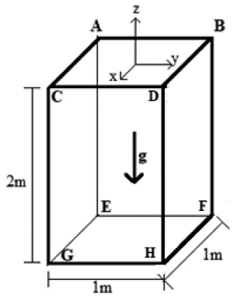
Figure 2 Straight prismatic bar under its weight.

Table 3 Displacement values for problem one

		−uz (mm)
	Z (m)	Sparseness = 20%	Sparseness = 60%	Sparseness = 100%	FEM	Analytical Solution
	−0.25	0.2424	0.2404	0.2397	0.2055	0.2345
	−0.50	0.4526	0.4487	0.4471	0.4141	0.4375
	−0.75	0.6291	0.6237	0.6211	0.5944	0.6100
Reference	−1.00	0.7729	0.7663	0.7627	0.7392	0.7500
[26]	−1.25	0.8845	0.8770	0.8726	0.8500	0.8600
	−1.50	0.9642	0.9561	0.9511	0.9285	0.9450
	−1.75	1.0119	1.0036	0.9982	0.9754	0.9900
	MAPE (%)	2.871	2.003	1.552	3.728
	−0.25	0.2397	0.2384	0.2365	0.2055	0.2345
	−0.50	0.4494	0.4455	0.4451	0.4141	0.4375
A3D8	−0.75	0.6261	0.6207	0.6185	0.5944	0.6100
	−1.00	0.7700	0.7640	0.7592	0.7392	0.7500
	−1.25	0.8815	0.8740	0.8697	0.8500	0.8600
	−1.50	0.9612	0.9528	0.9489	0.9285	0.9450
	−1.75	1.0009	1.0006	0.9963	0.9754	0.9900
	MAPE (%)	1.327	1.257	1.087	3.728
	−0.25	0.2389	0.2362	0.2340	0.2055	0.2345
	−0.50	0.4415	0.4387	0.4370	0.4141	0.4375
	−0.75	0.6154	0.6137	0.6110	0.5944	0.6100
	−1.00	0.7532	0.7521	0.7505	0.7392	0.7500
A3D20	−1.25	0.8700	0.8619	0.8605	0.8500	0.8600
	−1.50	0.9500	0.9467	0.9456	0.9285	0.9450
	−1.75	1.0007	0.9939	0.9915	0.9754	0.9900
	MAPE (%)	0.034	0.023	0.019	3.728

Table 4 Stress values for problem one

		σzz (kPa)
	Z (m)	Sparseness = 20%	Sparseness = 60%	Sparseness = 100%	FEM	Analytical Solution
	−0.25	36.34	36.02	35.88	36.30	35.6
	−0.50	30.87	30.60	30.44	31.81	30.0
	−0.75	25.57	25.35	25.19	25.91	25.0
Reference	−1.00	20.42	20.24	20.10	20.31	20.0
[23]	−1.25	15.32	15.18	15.06	15.08	15.0
	−1.50	10.20	10.13	10.04	10.01	10.0
	−1.75	5.11	5.07	5.02	5.00	5.0
	MAPE (%)	2.232	1.390	0.673	1.975
	−0.25	35.81	35.73	35.62	36.30	35.6
	−0.50	31.13	31.09	30.09	31.81	30.0
	−0.75	25.25	25.19	25.10	25.91	25.0
	−1.00	20.83	20.83	20.08	20.31	20.0
A3D8	−1.25	15.34	15.10	15.05	15.08	15.0
	−1.50	10.21	10.21	10.01	10.01	10.0
	−1.75	5.20	5.08	5.00	5.00	5.0
	MAPE (%)	0.25	0.13	0.08	1.975
	−0.25	35.72	35.62	35.61	36.30	35.6
	−0.50	31.11	30.81	30.08	31.81	30.0
	−0.75	25.20	25.10	25.09	25.91	25.0
	−1.00	20.74	20.62	20.07	20.31	20.0
A3D20	−1.25	15.25	15.07	15.04	15.08	15.0
	−1.50	10.20	10.10	10.00	10.01	10.0
	−1.75	5.10	5.02	5.00	5.00	5.0
	MAPE (%)	0.14	0.09	0.02	1.975

As it is seen in Tables 3 and 4, the suggested elements can predict the z-direction displacement and stress components with high accuracy compared to the previously presented elements. Furthermore, by increasing the node numbers and utilizing A3D20, the accuracy was even better. It is clear that the amount of MAPE was decreased by increasing sparseness values. In fact, the exact solution with the sparseness of 100% can be obtained by A3D20. The performances of both suggested elements in calculating the stress components were more accurate than the displacement components.

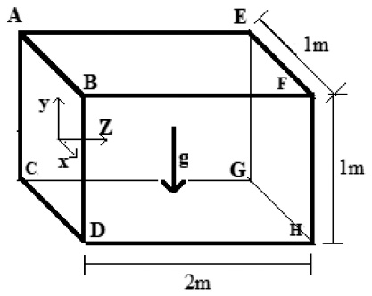
Figure 3 Bending effect of the cantilever beam.

Example 2: In this part, another benchmark problem is solved for demonstrating the performance of the new elements. The bending effect is considered in this example. Figure 3 shows a cantilever beam with u_xA = u_yA = u_zA = u_xB = u_yB = u_zB = u_xC = u_yC = u_zC = u_xD = u_yD = u_zD = 0. As it is seen in Figure 5, the structural dimensions are 1m × 2m × 1m. For this problem, the material properties are assumed to be E = 4 × 10⁷ Pa, ν = 0.25 and ρ = 2000 kg/m³.

To investigate the bending effect of this beam, the numerical results of deflection along the y-axis are calculated by the proposed method. These answers are compared with the finite element results and also with the outcomes of reference 23 in Table 5. As it was mentioned in the previous example, the same number of elements is used.

According to the obtained results, the computational accuracy of the authors’ formulation is high for this problem. The numerical solutions seem to converge when the degree of sparseness increases. In fact, the discrepancy between the suggested approach at full sparseness and FEM is only 0.05%.

Example 3: In this part, a cylinder with 10 m internal radius, 10 m thickness and 20 m height are considered. As it is shown in Figure 4, this structure is subjected under a centrifugal load. It should be reminded that this problem is solved with the following dimensionless material parameters, E = 2.1 × 10⁵, ν = 0.33 and ρ = 1. According to the body symmetry, only one-quarter of the cylinder domain needs to be analyzed. Based on Figure 4, appropriate symmetrical displacement constraints are also applied to the symmetric planes.

Table 5 Displacement outcomes of the cantilever beam

		uzz (mm)
	Z (m)	Sparseness = 20%	Sparseness = 60%	Sparseness = 100%	FEM
	0.25	−0.095	−0.094	−0.094	−0.093
	0.50	−0.246	−0.245	−0.243	−0.242
Reference [26]	0.75	−0.431	−0.429	−0.425	−0.424
	1.00	−0.634	−0.631	−0.625	−0.626
	1.25	−0.846	−0.842	−0.834	−0.837
	1.50	−1.060	−1.054	−1.044	−1.050
	1.75	−1.270	−1.263	−1.250	−1.258
A3D8	0.25	−0.095	−0.094	−0.093	−0.093
	0.50	−0.245	−0.243	−0.242	−0.242
	0.75	−0.427	−0.426	−0.425	−0.424
	1.00	−0.628	−0.626	−0.626	−0.626
	1.25	−0.839	−0.837	−0.837	−0.837
	1.50	−1.055	−1.051	−1.050	−1.050
	1.75	−1.262	−1.259	−1.258	−1.258
	0.25	−0.095	−0.094	−0.093	−0.093
	0.50	−0.244	−0.243	−0.242	−0.242
	0.75	−0.426	−0.425	−0.424	−0.424
A3D20	1.00	−0.627	−0.626	−0.625	−0.626
	1.25	−0.838	−0.837	−0.837	−0.837
	1.50	−1.053	−1.051	−1.050	−1.050
	1.75	−1.260	−1.259	−1.258	−1.258

It is obvious that for this structure, the stress fields are more complex than the two previous solved problems. The results of radial and hoop stresses at specified locations are arranged, respectively. All findings are obtained from the proposed method, available references [26] and FEM. They are represented in Tables 6 and 7. Similar to the former two examples, the MAPE of the suggested scheme reduces with increased sparseness. Once again, it is observed that good agreement between authors’ elements, and the available analytical solutions.

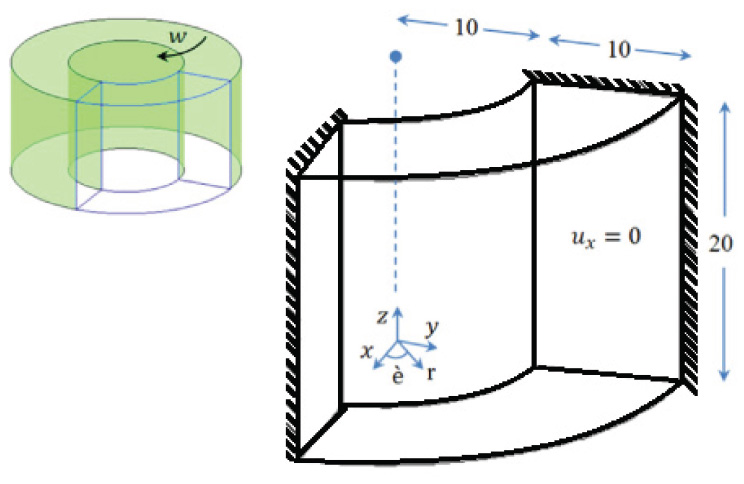
Figure 4 Thick cylinder subjected to centrifugal load.

For cylindrical shape problem, both A3D8 and A3D30 can calculate the displacement and stress components with high accuracy. However, the performance of A3D20 was better than A3D8. On the other hand, in this type of problems, the performance of proposed elements in order to calculate the radial stress components was more effective than hoop stress components.

Example 4: To analysis a complex state of stresses, the body in Figure 5 is solved under four circumstances of the loading. For the first case, it is assumed that 10 kg/m² the distributed load is applied in EFGH surface in the z-direction. It should be mentioned that the face ABCD is fixed in all cases, u_xA = u_yA = u_zA = u_xB = u_yB = u_zB = u_xC = u_yC = u_zC = u_xD = u_yD = u_zD = 0. Once again, the same dimensionless material parameters, E = 2.1 × 10⁵, ν = 0.3 and ρ = 1, are used for all different situations. After performing the required analysis, the obtained outputs are inserted in Table 8.

Example 5: In case two, 20 kg/m² the distributed load is applied in EFGH surface in the negative y-direction. In addition, 10 kg/m² force is applied in EFGH surface in the z-direction. All the obtained results for stress and displacement component in the z-direction with different sparseness from the central axis are represented in Tables 9 and 10.

Example 6: In case three, 30 kg/m² is applied to BFGH face in the x-direction. In addition, 20 kg/m² force is applied to EFGH face in the negative y-direction. Finally, 10 kg/m² force is applied to the EFGH surface in the z-direction. All the achieved results for the stress and displacement components, in the z-direction with different sparseness from the central axis, are represented in Tables 11 and 12.

Table 6 Radial stresses for the thick cylinder

		σr (kPa)
	r (m)	Sparseness = 20%	Sparseness = 60%	Sparseness = 80%	Sparseness = 100%	FEM	Analytical Solution
	11.25	2.723	2.221	2.424	2.340	2.434	2.367
	12.50	4.068	3.603	3.673	3.691	3.740	3.620
Reference	13.75	4.562	4.247	4.132	4.271	4.233	4.099
[26]	15.00	4.482	4.269	4.027	4.245	4.108	4.010
	16.25	4.005	3.789	3.489	3.751	3.568	3.484
	17.50	3.194	2.902	2.582	2.888	2.647	2.604
	18.75	1.942	1.652	1.357	1.684	1.442	1.430
	MAPE (%)	17.694	7.492	1.594	7.073	2.394
	11.25	2.461	2.432	2.384	2.370	2.434	2.367
	12.50	3.611	3.594	3.546	3.542	3.740	3.620
	13.75	4.228	4.213	4.154	4.152	4.233	4.099
	15.00	4.231	4.221	4.057	4.050	4.108	4.010
A3D8	16.25	3.594	3.571	3.502	3.497	3.568	3.484
	17.50	2.714	2.688	2.634	2.624	2.647	2.604
	18.75	1.602	1.482	1.454	1.450	1.442	1.430
	MAPE (%)	4.842	2.248	1.735	1.215	2.394
	11.25	2.432	2.401	2.371	2.365	2.434	2.367
	12.50	3.602	3.575	3.545	3.521	3.740	3.620
	13.75	4.209	4.182	4.152	4.100	4.233	4.099
	15.00	4.112	4.082	4.046	4.012	4.108	4.010
A3D20	16.25	3.555	3.530	3.491	3.485	3.568	3.484
	17.50	2.695	2.677	2.612	2.608	2.647	2.604
	18.75	1.503	1.473	1.441	1.433	1.442	1.430
	MAPE (%)	0.815	0.118	0.017	0.008	2.394

Table 7 Hoop stresses for the thick cylinder

		σt (kPa)
	r (m)	Sparseness = 20%	Sparseness = 60%	Sparseness = 100%	FEM	Analytical Solution
	11.25	33.88	28.69	29.92	31.48	30.66
	12.50	29.71	26.29	27.00	28.24	27.47
Reference	13.75	26.27	24.24	24.53	25.55	24.86
[23]	15.00	23.27	22.45	22.38	23.21	22.61
	16.25	20.51	20.84	20.43	21.10	20.60
	17.50	17.96	19.36	18.63	19.12	18.74
	18.75	15.78	18.03	17.05	17.21	16.97
	MAPE (%)	5.542	3.520	1.200	2.392
	11.25	32.11	31.89	31.24	31.48	30.66
	12.50	29.37	29.06	28.84	28.24	27.47
	13.75	26.17	25.89	25.43	25.55	24.86
A3D8	15.00	23.76	23.57	23.11	23.21	22.61
	16.25	21.73	21.42	21.00	21.10	20.60
	17.50	19.82	19.48	19.54	19.12	18.74
	18.75	18.09	17.86	17.43	17.21	16.97
	MAPE (%)	3.170	2.407	1.7942	2.392
	11.25	31.42	31.03	30.67	31.48	30.66
	12.50	28.06	27.84	27.50	28.24	27.47
	13.75	25.67	25.26	24.89	25.55	24.86
A3D20	15.00	23.21	22.97	22.67	23.21	22.61
	16.25	21.19	20.91	20.65	21.10	20.60
	17.50	19.45	19.01	18.80	19.12	18.74
	18.75	17.59	17.28	17.00	17.21	16.97
	MAPE (%)	0.421	0.122	0.038	2.392

According to the obtained results, the computational accuracy of the authors’ formulation is high for this problem. The numerical solutions seem to converge when the degree of sparseness increases and the discrepancy between the suggested approach at full sparseness and FEM is only 0.07%.

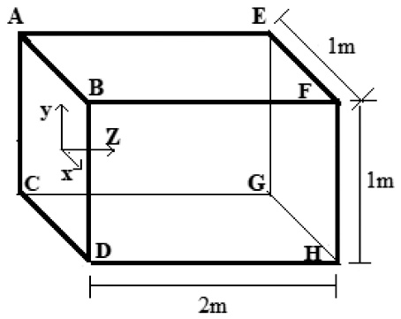
Figure 5 Body under four different loadings.

Table 8 Stress consequences for case one

		σzz (kPa)
	Z (m)	Sparseness = 20%	Sparseness = 60%	Sparseness = 100%	FEM	Analytical Solution
	0.25	46.52	46.38	46.13	46.30	45.71
	0.50	41.91	41.81	41.52	41.81	40.12
	0.75	35.85	35.74	35.66	35.91	35.74
	1.00	31.39	31.15	30.95	30.31	30.27
A3D8	1.25	25.81	25.72	25.49	25.08	25.21
	1.50	20.82	20.68	20.45	20.01	20.01
	1.75	10.43	10.24	10.19	10.00	10.00
	MAPE (%)	3.342	2.423	0.680	1.975
	0.25	45.93	45.78	45.63	46.30	45.71
	0.50	41.25	41.06	40.10	41.81	40.12
	0.75	35.66	35.50	35.67	35.91	35.74
	1.00	30.95	30.83	30.17	30.31	30.27
A3D20	1.25	25.49	25.10	25.19	25.08	25.21
	1.50	20.45	20.21	20.01	20.01	20.01
	1.75	10.19	10.08	10.00	10.00	10.00
	MAPE (%)	0.681	0.171	0.082	1.975

Table 9 Stress consequences for case two

		σzz (kPa)
	Z (m)	Sparseness = 20%	Sparseness = 60%	Sparseness = 100%	FEM	Analytical Solution
	0.25	51.58	51.34	51.13	51.30	50.71
	0.50	46.83	46.38	46.24	46.81	45.12
	0.75	41.38	41.07	40.86	40.91	40.74
	1.00	36.49	36.22	35.94	35.31	35.27
A3D8	1.25	30.98	30.72	30.48	30.08	30.21
	1.50	25.73	25.48	25.23	25.01	25.01
	1.75	15.54	15.38	15.17	15.00	15.00
	MAPE (%)	2.420	1.973	1.413	2.175
	0.25	50.92	50.75	50.69	51.30	50.71
	0.50	46.24	46.13	45.09	46.81	45.12
	0.75	40.86	40.74	40.69	40.91	40.74
A3D20	1.00	35.94	35.83	35.16	35.31	35.27
	1.25	30.48	30.21	30.17	30.08	30.21
	1.50	25.23	25.09	25.01	25.01	25.01
	1.75	15.17	15.08	15.00	15.00	15.00
	MAPE (%)	0.412	0.137	0.071	2.175

Table 10 Displacement outcomes for case two

		uz (mm)
	Z (m)	Sparseness = 20%	Sparseness = 60%	Sparseness = 100%	FEM	Analytical Solution
	0.25	0.3501	0.3475	0.3457	0.3055	0.3345
	0.50	0.5591	0.5573	0.5551	0.5141	0.5375
	0.75	0.7771	0.7746	0.7721	0.6944	0.7100
	1.00	0.8810	0.8786	0.8768	0.8392	0.8500
A3D8	1.25	0.9921	0.9897	0.9872	0.9500	0.9600
	1.50	1.0772	1.0689	1.0662	1.0285	1.0450
	1.75	1.1221	1.1190	1.1171	1.1754	1.1100
	MAPE (%)	4.015	3.487	3.007	3.728
	0.25	0.3426	0.3402	0.3354	0.3055	0.3345
	0.50	0.5525	0.5485	0.5471	0.5141	0.5375
	0.75	0.7293	0.7234	0.7111	0.6944	0.7100
	1.00	0.8731	0.8662	0.8527	0.8392	0.8500
A3D20	1.25	0.9847	0.9770	0.9616	0.9500	0.9600
	1.50	1.0644	1.0588	1.0511	1.0285	1.0450
	1.75	1.1152	1.1133	1.1112	1.1754	1.1100
	MAPE (%)	2.752	1.543	0.885	3.728

Table 11 Stress consequences for case three

		σzz (kPa)
	Z (m)	Sparseness = 20%	Sparseness = 60%	Sparseness = 100%	FEM	Analytical Solution
	0.25	63.38	63.12	62.95	62.30	62.41
	0.50	58.72	58.59	58.32	57.41	56.80
	0.75	52.93	52.71	52.51	52.71	51.74
	1.00	48.46	48.11	47.94	47.21	47.17
A3D8	1.25	43.03	42.84	42.51	41.18	41.32
	1.50	37.61	37.35	37.19	36.01	36.01
	1.75	27.85	27.64	27.13	26.00	26.00
	MAPE (%)	4.008	3.257	2.943	2.575
	0.25	62.72	62.54	62.38	62.30	62.41
	0.50	58.04	57.29	56.79	57.41	56.80
	0.75	52.16	51.91	51.80	52.71	51.74
	1.00	47.74	47.37	47.18	47.21	47.17
A3D20	1.25	42.28	41.61	41.36	41.18	41.32
	1.50	37.13	37.00	36.01	36.01	36.01
	1.75	27.02	26.18	26.00	26.00	26.00
	MAPE (%)	1.373	0.137	0.090	2.575

Table 12 Displacement outcomes for case three

		uz (mm)
	Z (m)	Sparseness = 20%	Sparseness = 60%	Sparseness = 100%	FEM	Analytical Solution
	0.25	0.4705	0.4672	0.4657	0.4255	0.4545
	0.50	0.6819	0.6785	0.6762	0.6241	0.6675
	0.75	0.8469	0.8443	0.8412	0.8144	0.8300
	1.00	0.9883	0.9861	0.9848	0.9592	0.9700
A3D8	1.25	1.1225	1.1198	1.1171	1.0700	1.0800
	1.50	1.1834	1.1799	1.1768	1.1485	1.1650
	1.75	1.2458	1.2425	1.2396	1.2954	1.2300
	MAPE (%)	4.110	3.824	3.183	3.918
	0.25	0.4613	0.4578	0.4553	0.4255	0.4545
	0.50	0.6726	0.6699	0.6671	0.6241	0.6675
	0.75	0.8384	0.8337	0.8310	0.8144	0.8300
	1.00	0.9829	0.9742	0.9707	0.9592	0.9700
A3D20	1.25	1.1145	1.1082	1.0813	1.0700	1.0800
	1.50	1.1742	1.1676	1.1654	1.1485	1.1650
	1.75	1.2369	1.2336	1.2300	1.2954	1.2300
	MAPE (%)	2.793	1.513	0.072	3.918

Table 13 Stress consequences for case four

		σzz (kPa)
Z (m)	Sparseness = 20%	Sparseness = 60%	Sparseness = 100%	FEM	Analytical Solution
	0.25	51.43	51.19	50.81	50.18	50.29
	0.50	46.77	46.38	46.13	45.29	45.68
	0.75	40.96	40.69	40.38	39.59	39.62
	1.00	36.29	36.00	35.85	35.08	35.05
A3D8	1.25	31.04	30.75	30.49	29.06	29.20
	1.50	26.17	25.84	25.37	24.84	24.84
	1.75	16.09	15.88	15.29	14.88	14.88
	MAPE (%)	2.138	1.275	0.840	1.635
	0.25	50.60	50.41	50.20	50.18	50.29
	0.50	45.98	45.77	45.67	45.29	45.68
	0.75	40.02	39.79	39.70	39.59	39.62
	1.00	35.62	35.41	35.06	35.08	35.05
A3D20	1.25	30.16	29.75	29.14	29.06	29.20
	1.50	25.01	24.84	24.84	24.84	24.84
	1.75	15.01	14.88	14.88	14.88	14.88
	MAPE (%)	0.371	0.257	0.081	1.635

Example 7: In case four, the structure presented Figure 5 is solved under the concentrate couple forces applied in the middle of EF and GH in both negative and positive z-direction. These couple forces are 10 kg. For this situation, the surface ABCD is also fixed, which leads to u_xA = u_yA = u_zA = u_xB = u_yB = u_zB = u_xC = u_yC = u_zC = u_xD = u_yD = u_zD = 0. Tables 13 and 14 demonstrate the obtained results of stress and displacement along the z-direction.

As it is seen in Tables 13 and 14, the presented elements can fore-cast the z-direction displacement and stress components with high accuracy compared to the FEM. Furthermore, by increasing the number of nodes and using A3D20, the accuracy was raised. Besides, the amount of MAPE was decreased by increasing the sparseness content. This clearly proved that the analytical responses can be achieved when A3D20 was used since the sparseness was 100%. It was demonstrated that for the complex stress cases, the performances of both A3D8 and A3D20, in calculating the stress components, were more accurate than finding the displacement components.

Table 14 Displacement outcomes for case four

		uz (mm)
Z (m)	Sparseness = 20%	Sparseness = 60%	Sparseness = 100%	FEM	Analytical Solution
	0.25	0.4713	0.4685	0.4653	0.4255	0.4545
	0.50	0.6759	0.6773	0.6749	0.6241	0.6675
	0.75	0.8528	0.8409	0.8381	0.8144	0.8300
	1.00	0.9950	0.9751	0.9724	0.9592	0.9700
A3D8	1.25	1.0071	1.0973	1.0942	1.0700	1.0800
	1.50	1.1882	1.1797	1.1768	1.1485	1.1650
	1.75	1.2345	1.2468	1.2432	1.2954	1.2300
	MAPE (%)	3.793	2.513	2.008	3.918
	0.25	0.4614	0.4584	0.4553	0.4255	0.4545
	0.50	0.6726	0.6702	0.6671	0.6241	0.6675
	0.75	0.8372	0.8347	0.8311	0.8144	0.8300
	1.00	0.9692	0.9663	0.9617	0.9592	0.9700
A3D20	1.25	1.0905	1.0870	1.0836	1.0700	1.0800
	1.50	1.1742	1.1711	1.1687	1.1485	1.1650
	1.75	1.2391	1.2363	1.2342	1.2954	1.2300
	MAPE (%)	1.793	0.998	0.655	3.918

Conclusion

In this paper, a novel scheme for developing two stress-based elements was proposed. Both suggested elements had three-dimensional isoparametric shapes, which are suitable for meshing irregular domain. According to comprehensive numerical studies, these formulations can solve the three-dimensional problem accurately. Indeed, the proposed elements can give precise responses for both displacement and stress. As it was demonstrated in this article, the entire element construction procedure was different from those of the traditional models. Based on this study, the following issues can be addressed:

• (1) Airy stress function was taken as the functional variable, and by minimizing the complementary energy functional, proper formulation was established and two new three-dimensional isoparametric elements were generated.
• (2) To demonstrate the abilities of the new suggested elements, a variety of the famous benchmark problems were solved.
• (3) Findings clearly showed that these elements can give both good displacements and stress responses.
• (4) Based on the numerical experiences, the orders of accuracy in these two new elements were A3D8 and A3D20.
• (5) Accuracy of proposed elements in order to calculate the stress components was more than the displacement components and was more precise than those presented by previous investigations.
• (6) For cylindrical structures, both A3D8 and A3D30 could calculate the displacement and stress components with high accuracy. However, the performance of A3D20 was more than A3D8. On the other hand, in this type of problems, the performance of proposed elements in order to calculate the radial stress components was more effective than the hoop stress components.

Funding

This study was not funded by any company.

Conflict of Interest

The authors declare that they have no conflict of interest.

References

[1] Fu, X. R., Cen, S., Li, C. F. and Chen, X. M. (2008). “Analytical trial function method for the development of new 8-node plane element based on the variational principle containing Airy stress function”, Engineering Computations: International Journal for Computer-Aided Engineering and Software, Vol. 27, No. 4, 2010, pp. 442–463.

[2] Lee, N. S. and Bathe, K. J. (1993). “Effects of element distortion on the performance of isoparametric elements”, International Journal for Numerical Methods in Engineering, Vol. 36, pp. 3553–3376.

[3] Kikuchi, F., Okabe, M. and Fujio, H. (1999). “Modification of the 8-node serendipity element”, Computer Methods in Applied Mechanics and Engineering, Vol. 179, pp. 91–109.

[4] Li, L. X., Kunimatsu, S., Han, X. P. and Xu, S. Q. (2004). “The analysis of interpolation precision of quadrilateral elements”, Finite Elements in Analysis and Design, Vol. 41, pp. 91–108.

[5] Rajendran, S. and Liew, K. M. (2003). “A novel unsymmetric 8-node plane element immune to mesh distortion under a quadratic displacement field”, International Journal for Numerical Methods in Engineering, Vol. 58, pp. 1713–1748.

[6] Li, C. J. and Wang, R. H. (2006). “A new 8-node quadrilateral spline finite element”, Journal of Computational and Applied Mathematics, Vol. 195, pp. 54–65.

[7] Long, Y. Q. and Xu, Y. (1994). “Generalized conforming triangular membrane element with vertex rigid rotational freedom”, Finite Elements in Analysis and Design, Vol. 17, pp. 259–271.

[8] Cen, S., Chen, X. M. and Fu, X. R. (2007). “Quadrilateral membrane element family formulated by the quadrilateral area coordinate method”, Computer Methods in Applied Mechanics and Engineering, Vol. 196, Nos. 41–44, pp. 4337–4353.

[9] Soh, A. K., Long, Y. Q. and Cen, S. (2000). “Development of eight-node quadrilateral membrane elements using the area coordinates method”, Computational Mechanics, Vol. 25, No. 4, pp. 376–84.

[10] Cen, S., Fu, X. R. and Zhou, M. J. (2011). “8- and 12-node plane hybrid stress-function elements immune to severely distorted mesh containing elements with concave shapes”, Computer Methods in Applied Mechanics and Engineering, Vol. 200, pp. 2321–2336.

[11] Cen, S., Zhou, M. J. and Fu, X. R. (2011). “A 4-node hybrid stress-function (HS-F) plane element with drilling degrees of freedom less sensitive to severe mesh distortions”, Computers & Structures, Vol. 89, Nos. 5–6, pp. 517–528.

[12] Cen, S., Fu, X. R., Zhou, G. H., Zhou, M. J. and Li, C. F. (2011). “Shape-free finite element method: The plane hybrid stress-function (HS-F) element method for anisotropic materials”, SCIENCE CHINA, Physics, Mechanics & Astronomy, Vol. 54, No. 4, pp. 653–665.

[13] Zhou, P. and Cen, S. (2015). “A novel shape-free plane quadratic polygonal hybrid stress-function element”, Mathematical Problems in Engineering, 491325.

[14] Rezaiee-Pajand, M. and Karimipour, A. (2019). “Three stress-based triangular elements”, Engineering with Computers, Vol. 20, No. 10, pp. 1–12.

[15] Artioli, E., Miranda, E. D., Lovadina, C. and Patruno, L. (2017). “A stress/displacement Virtual Element method for plane elasticity problems”, Computer Methods in Applied Mechanics and Engineering, Vol. 325, pp. 155–174.

[16] Rezaiee-Pajand, M. and Karkon, M. (2016). “Geometrical Nonlinear Analysis of Plane Problems by Corotational Formulation”, Journal of Engineering Mechanics, Vol. 142, No. 10, p. 04016073.

[17] Nieh, J. Y., Huang, C. S. and Tseng, Y. P. (2003). “An analytical solution for in-plane free vibration and stability of loaded elliptic arches”, Computers & Structures, Vol. 81, No. 13, pp. 1311–1327.

[18] Serra, M. (1994). “Optimal arch: Approximate analytical and numerical solutions”, Computers & Structures, Vol. 52, No. 6, 17 September, pp. 1213–1220.

[19] HarikGhassan, I. E. and Salamoun, L. (1988). “The analytical strip method of solution for stiffened rectangular plates”, Computers & Structures, Vol. 29, No. 2, pp. 283–291.

[20] Karttunen, A. T., Hertzen, R., Reddy, J. N. and Romanoff, J. (2018). “Shear deformable plate elements based on exact elasticity solution”, Computers & Structures, Vol. 200, 15 April, pp. 21–31.

[21] Arya, V. K. (1989). “Analytical and finite element solutions of some problems using a viscoelastic model”, Computers & Structures, Vol. 33, No. 4, pp. 957–967.

[22] Zhang, Z., Dissanayake, D., Saputra, A., Wu, D. and Song, C. (2018). “Three-dimensional damage analysis by the scaled boundary finite element method”, Computers & Structures, Vol. 206, 15 August, pp. 1–17.

[23] Shang, H. Y., Machado, R. D. and Filho, J. E. A. (2016). “Dynamic analysis of Euler-Bernoulli beam problems using the Generalized Finite Element Method”, Computers & Structures, Vol. 173, September, pp. 109–122.

[24] Shang, Y., Cen, S. and Zhou, M. J. (2018). “8-node unsymmetric distortion-immune element based on Airy stress solutions for plane orthotropic problems”, Acta Mechanica, Vol. 45, pp. 234–250.

[25] Shankar, L. S., Rajthilak, S. and Saravanan, U. (2016). “Numerical technique for solving truss and plane problems for a new class of elastic bodies”, Acta Mechanica, Vol. 27, pp. 128–157.

[26] Barber, J. R. (2006). “Three-dimensional elasticity problems for the prismatic bar”, Proceeding of The Royal Society, Vol. 462, pp. 1877–1896.

Biographies

Mohammad Rezaiee-Pajand received his PhD in Structural Engineering from University of Pittsburgh, Pittsburgh, PA, USA. He is currently a Professor at Ferdowsi University of Mashhad (FUM), Mashhad, Iran. His research interests are: Nonlinear structural analysis, Finite element method, Dynamic relaxation method, Composite structures, Structural vibration, Structural dynamics, Nonlinear solvers, Time integration, Plate and shell, Computational plasticity, Structural optimization and Numerical techniques.

Arash Karimipour attended the University of Ilam, where he received his B.Sc. in Civil Engineering in 2015. Then, he obtained M.Sc. degree in structural Engineering from the Ferdowsi University of Mashhad, Iran, in 2017. Arash has started Ph.D. program at the University of Texas at El Paso since fall 2019. His research interests are: Analysis and design of concrete structures, Finite element method, Experimental and numerical simulation of reinforced concrete pavement.

European Journal of Computational Mechanics, Vol. 28_5, 373–410.
doi: 10.13052/ejcm2642-2085.2851
© 2020 River Publishers