Two Ways of Solving System of Nonlinear Structural Equations

Mohammad Rezaiee-Pajand, Rahele Naserian and Hossein Afsharimoghadam

Department of Civil Engineering, Ferdowsi University of Mashhad, Mashhad, Iran

Email: rezaiee@um.ac.ir

* Corresponding Author

Received 09 February 2019; Accepted 03 December 2019; Publication 14 January 2020

Abstract

By applying the inner product of vectors, two objective functions are found. These vectors are taken from the structural equilibrium path. Via minimizing these functions, with respect to the load incremental parameter and the angle between particular vectors, two new constraint equalities are achieved. Since the scheme of authors is general, three more constraints are also reached. These formulations are similar to the previous presented nonlinear solvers, which confirm the legitimacy of new procedure. Afterward, several numerical tests are performed to prove the ability of the proposed techniques. Findings show that the new algorithms are capable in passing the load and displacement limit points of the various benchmark problems with severe nonlinear behaviors. Based on the number of increments and iterations and also the total analysis duration, the suggested methods have the maximum rapid convergence rate, in comparison to the normal plane, the updated normal plane and the cylindrical arc length strategies.

Keywords: Constraint equality, objective function, load incremental parameter, structural equilibrium path, limit points.

1 Introduction

The most popular solution methods used in the nonlinear finite element analysis are incremental-iterative techniques. In the linear incremental process, the load-displacement path is approximated piecewise linear. Under this assumption, the residual forces between external and internal nodal loads are produced [1]. In this case, an iteration procedure is necessary to eliminate the residual forces in each incremental step and to obtain more accurate results. In each step of incremental-iterative analysis, the following equation should be solved:

$$R(x,\lambda )=\lambda P-R^{\text{int}}(x)$$

(1)

Where the displacement vector and load incremental parameter are shown by x and λ, respectively. Furthermore, the external load, internal load, and residual force vectors are denoted by P, R^int(x), and R(x, λ), correspondingly. In the direct iteration method, entire loads are applied in a single step [2]. It should be noted that in the geometric nonlinear analysis, the internal loads and stiffness matrix are nonlinear functions of the nodal displacements. To perform analysis, the nodal displacement in each iteration is decomposed into the displacements induced by the external load, $\delta \widehat{x}$, and the residual force, $\delta \overline{x}$, [3]:

$$\delta x=\delta \overline{x}+\delta \lambda \delta \widehat{x},S\delta \overline{x}=R,S\delta \widehat{x}=P$$

(2)

In Equation (2), S indicates the tangential stiffness matrix. For a structure with N degrees of freedom, there are N equations with N + 1 unknowns which are the incremental displacement vector components and load incremental parameter. So far, several different versions of incremental-iterative solutions have been created based on how to control the load incremental parameter, and the way iterations are carried out within an incremental step. Riks and Ramm suggested the normal plane [4], and the updated normal plane process [5], respectively. In order to find the load incremental parameter in each iteration, Bergan minimized the residual force [6]. Furthermore, Crisfield formulated the cylindrical arc length algorithm [7].

By considering other views, researchers suggested various approaches by minimizing the residual displacement [8], and the unbalanced perimeter and residual area [9, 10]. Additionally, Rezaiee-Pajand and Afsharimoghadam obtained new constraints for geometric nonlinear analysis by optimization techniques [11]. The generalized displacement control method (GDCM) is an efficient technique for tracing the static equilibrium path [12]. This technique can trace the load, and displacement limit points. Cardoso and Fonseca identified that GDCM can be expressed as an orthogonal arc length approach [13]. Moreover, Leon et al. provided the modification of GDCM [14]. It should be reminded; this technique is more robust than the standard GDCM for capturing equilibrium paths in the region with intensive curvature. Note that the normal flow algorithm traces the lines perpendicular to Davidenko’s flow in each iteration [15]. Saffari et al. improved this method [16].

The dynamic relaxation technique is another way of solving the structural nonlinear equations [17–21]. In this procedure, the static equilibrium equations were solved in a fictitious dynamic space. In other words, the dynamic relaxation method is an explicit approach for solving the simultaneous systems of equations. In this scheme, the fictitious mass and damping are added to the static governing equations, and an artificial dynamic system is built [22–24]. By this procedure, various nonlinear structural analyses have been performed in recent years [25–29].

In addition, there are some other techniques accessible for the nonlinear structural analysis. In 2011, Saffari and Mansouri employed two-point approach with fourth order convergence for assessing the nonlinear behavior of structures [30]. In another study, an accelerated incremental tactic with the order convergence of eight was achieved by mixing several efficient functions in the normal flow technique [31]. Three brief reviews of nonlinear solution techniques were presented by researchers [32–34]. Furthermore, Torkamani and Sheih, and Rezaiee-Pajand and Naserian analyzed the geometric nonlinear behavior of truss and frame structures by using higher-order stiffness matrices [35–37]. In these methods, all the linear and nonlinear components of the strain vector were deployed in incremental static equations. Recently, a technique without incremental solution predictor step was introduced [38], and also three constraint equalities based on the residual factors were proposed [39].

In this paper, two new formulas are suggested for computing the load incremental parameter in the iterative procedure. These relations are obtained by optimizing the objective functions created from the inner product of the residual vectors. At first, the cylindrical arc length scheme is introduced briefly. Then, new formulations are presented. For this purpose, the inner product of the residual vectors is written in terms of the load incremental parameter and angle between two vectors. By minimizing the resulted functions, two novel constraint equations are obtained. Afterward, the robustness of the proposed methods is evaluated by performing several numerical tests. To confirm the solution validity process, the suggested procedures are compared with the techniques of the other researches, such as the cylindrical arc length (CAL), the normal plane (NP), the updated normal plane (UNP) schemes, and also Abaqus software. To demonstrate the advantage of novel formulations, the total number of increments and iterations required for the analysis of each example are shown. It should be emphasized that three more constraints are also found during the process of developing the required mathematical relations. These constraints belonged to the famous former nonlinear solvers. As a result; this event can be called another way of confirming the legitimacy of new procedure.

2 Cylindrical Arc Length Technique

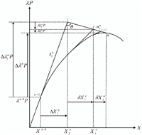
In this algorithm, the distances of all iterative points of each increment from the previous equilibrium status are kept constant [7]. This distance is named length factor (L_n). Figure 1 shows this process in the analysis of a single degree of freedom structure. Accordingly, the constraint equation of the cylindrical arc length strategy can be expressed as the next line:

$${\overrightarrow{t}}_{i+1}^n\cdot {\overrightarrow{t}}_{i+1}^n={(L_n)}^2$$

(3)

In this equality, ${\overrightarrow{t}}_{i+1}^n$ is the vector connecting the (n − 1)th point of the equilibrium path to the (i + 1)th point of the iteration path. It should be added that Crisfield ignored the load component against the displacement one, as follows:

$$\Delta x_{i+1}^{n^T}\Delta x_{i+1}^n={(L_n)}^2$$

(4)

Based on Figure 1, the current relationship can be rewritten as the next form:

$${(\Delta x_i^n+\delta x_i^n)}^T(\Delta x_i^n+\delta x_i^n)={(L_n)}^2$$

(5)

In iteration steps, inserting Equation (2) into Equation (5) and simplifying the resulted equality, lead to the subsequent second-order relationship:

$$a{(\delta {\lambda }_i^n)}^2+b(\delta {\lambda }_i^n)+c=0$$

(6)

The constant coefficients used in the current equation are defined in the following forms:

$$a={(\delta {\widehat{x}}_i^n)}^T(\delta {\widehat{x}}_i^n)$$

(7)

$$b=2{(\Delta x_i^n+\delta {\overline{x}}_i^n)}^T(\delta {\widehat{x}}_i^n)$$

(8)

$$c=2{(\Delta x_i^n+\delta {\overline{x}}_i^n)}^T(\Delta x_i^n+\delta {\overline{x}}_i^n)-L_n^2$$

(9)

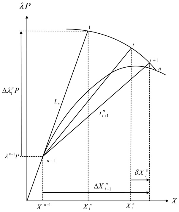
Figure 1 The general procedure of the cylindrical arc length technique.

After determining these coefficients and solving Equation (6), the next two roots will be achieved for the load incremental parameter:

$$\{\begin{array}{c}\begin{array}{c}\delta {\lambda }_{i,1}^n\\ \delta {\lambda }_{i,2}^n\end{array}=-\frac{b}{2a}\pm \sqrt{{\left(\frac{b}{2a}\right)}^2-\frac{c}{a}}\end{array}$$

(10)

If the coming condition is satisfied, the obtained roots are real:

$$\Delta =b^2-4ac>0$$

(11)

The root which is closer to the last iteration point, should be selected. The distance between the roots and the last iteration point can be obtained via the following Equation (40):

$$\Delta x_{i+1}^n\Delta x_i^n={(\Delta x_i^n+\delta {\overline{x}}_i^n+\delta {\lambda }_i^n\delta {\widehat{x}}_i^n)}^T\Delta x_i^n$$

(12)

This control formula prevents the load-displacement path returns to itself. If Δ in Equation (11) equals to zero, only one root exists. When Δ becomes negative, the obtained roots will be complex, and they are not acceptable. To overcome this difficulty, the value of the length factor is reduced, and the problem is solved again.

3 Optimized Normal Plane Strategy

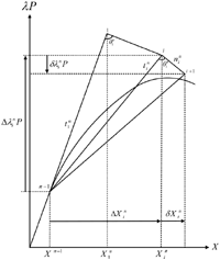
In this technique, the vector of the iterative points location, ${\overrightarrow{n}}_i^n$, constructs various angles with the tangent vector to the previous equilibrium point, ${\overrightarrow{t}}_1^n$. The process of the optimized normal plane (ONP) approach for a single degree of freedom system is shown in Figure 2. Hence, the constraint equation can be written as the subsequent equality:

$${\overrightarrow{t}}_1^n\cdot {\overrightarrow{n}}_i^n=\left|t_1^n\right|\left|n_i^n\right|Cos\theta$$

(13)

$${\overrightarrow{t}}_1^n=(\Delta x_1^n,\Delta {\lambda }_1^{n}P)$$

(14)

$${\overrightarrow{n}}_i^n=(\delta x_i^n,\delta {\lambda }_i^{n}P)$$

(15)

In these relations, the angle between ${\overrightarrow{n}}_i^n$ and ${\overrightarrow{t}}_1^n$ is shown by θ. According to the equalities (14) and (15), the inner product of these vectors leads to the succeeding result:

$$\begin{array}{l}(\Delta x_1^n,\Delta {\lambda }_1^{n}P)\cdot (\delta x_i^n,\delta {\lambda }_i^{n}P)=\left(\sqrt{\Delta x_1^{n^T}\Delta x_1^n+{(\Delta {\lambda }_1^n)}^2{P}^{T}P}\right)\hfill \\ \left(\sqrt{\delta x_i^{n^T}\delta x_i^n+{(\delta {\lambda }_i^n)}^2{P}^{T}P}\right)\mathit{Cos}\theta \hfill \end{array}$$

(16)

By inserting Equation (2) into the equality (16), the constraint equation can be obtained as follows:

$$\begin{array}{l}\delta {\lambda }_i^n(\Delta x_1^{n^T}\delta {\widehat{x}}_i^n+\Delta {\lambda }_1^n{P}^{T}P)+\Delta x_1^{n^T}\delta {\overline{x}}_i^n\hfill \\ =\left(\sqrt{\begin{array}{l}[\Delta x_1^{n^T}\Delta x_1^n+{(\Delta {\lambda }_1^n)}^2{P}^{T}P]\hfill \\ [{(\delta {\overline{x}}_i^n+\delta {\lambda }_i^n\delta {\widehat{x}}_i^n)}^T(\delta {\overline{x}}_i^n+\delta {\lambda }_i^n\delta {\widehat{x}}_i^n)+{(\delta {\lambda }_i^n)}^2{P}^{T}P]\hfill \end{array}}\right)\mathit{Cos}\theta \hfill \end{array}$$

(17)

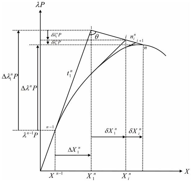
Figure 2 The general procedure of optimized normal plane strategy.

Squaring both sides of Equation (17), leads to the next relation:

$$\begin{array}{l}{(\delta {\lambda }_i^n)}^2[{(\Delta x_1^{n^T}\delta {\widehat{x}}_i^n+\Delta {\lambda }_1^n{P}^{T}P)}^2-Co{s}^2\theta (\delta {\widehat{x}}_i^{n^T}\delta {\widehat{x}}_i^n+P^{T}P)\hfill \\ (\Delta x_1^{n^T}\Delta x_1^n+{(\Delta {\lambda }_1^n)}^2{P}^{T}P)]\hfill \\ +2(\delta {\lambda }_i^n)[(\Delta x_1^{n^T}\delta {\overline{x}}_i^n)(\Delta x_1^{n^T}\delta {\widehat{x}}_i^n+\Delta {\lambda }_1^n{P}^{T}P)\hfill \\ -Co{s}^2\theta (\delta {\overline{x}}_i^{n^T}\delta {\widehat{x}}_i^n)(\Delta x_1^{n^T}\Delta x_1^n+{(\Delta {\lambda }_1^n)}^2{P}^{T}P)]\hfill \\ +[{(\Delta x_1^{n^T}\delta {\overline{x}}_i^n)}^2-Co{s}^2\theta (\delta {\overline{x}}_i^{n^T}\delta {\overline{x}}_i^n)\hfill \\ (\Delta x_1^{n^T}\Delta x_1^n+{(\Delta {\lambda }_1^n)}^2{P}^{T}P)]=0\hfill \end{array}$$

(18)

As a result, the inner product of the vector passing through the iterative points and the tangent vector to the previous equilibrium point, leads to an objective function with two variables. To achieve the constraint equation, this function is optimized based on the angle variable between the aforesaid vectors, and also the load incremental parameter. At the first stage, function (18) is minimized with respect to $\delta {\lambda }_i^n$:

$$\begin{array}{l}(\delta {\lambda }_i^n)[{(\Delta x_1^{n^T}\delta {\widehat{x}}_i^n+\Delta {\lambda }_1^n{P}^{T}P)}^2-{\mathit{Cos}}^2\theta (\delta {\widehat{x}}_i^{n^T}\delta {\widehat{x}}_i^n+P^{T}P)\hfill \\ (\Delta x_1^{n^T}\Delta x_1^n+{(\Delta {\lambda }_1^n)}^2{P}^{T}P)]\hfill \\ +[(\Delta x_1^{n^T}\delta {\overline{x}}_i^n)(\Delta x_1^{n^T}\delta {\widehat{x}}_i^n+\Delta {\lambda }_1^n{P}^{T}P)-{\mathit{Cos}}^2\theta (\delta {\overline{x}}_i^{n^T}\delta {\widehat{x}}_i^n)\hfill \\ (\Delta x_1^{n^T}\Delta x_1^n+{(\Delta {\lambda }_1^n)}^2{P}^{T}P)]=0\hfill \end{array}$$

(19)

On the other hand, by squaring both sides of Equation (17), the next value for Cos²θ can be achieved:

$${\mathit{Cos}}^2\theta =\frac{{[\delta {\lambda }_i^n(\Delta x_1^{n^T}\delta {\widehat{x}}_i^n+\Delta {\lambda }_1^n{P}^{T}P)+\Delta x_1^n\delta {\overline{x}}_i^n]}^2}{\begin{array}{l}[\Delta x_1^{n^T}\Delta x_1^n+{(\Delta {\lambda }_1^n)}^2{P}^{T}P]\hfill \\ [{(\delta {\overline{x}}_i^n+\delta {\lambda }_i^n\delta {\widehat{x}}_i^n)}^T(\delta {\overline{x}}_i^n+\delta {\lambda }_i^n\delta {\widehat{x}}_i^n)+{(\delta {\lambda }_i^n)}^2{P}^{T}P]\hfill \end{array}}$$

(20)

Substituting Cos²θ from Equation (20) into Equation (19), and performing some algebraic simplifications lead to the subsequent quadratic constraint relation:

$$a{(\delta {\lambda }_i^n)}^2+b(\delta {\lambda }_i^n)+c=0$$

(21)

The constant coefficients used in the current equation are given in the below lines:

$$\begin{array}{l}a=-{(\Delta {\lambda }_1^n)}^2\delta {\widehat{x}}_i^{n^T}\delta {\overline{x}}_i^n{P}^{T}P-\Delta {\lambda }_1^n\delta {\widehat{x}}_i^{n^T}\delta {\widehat{x}}_i^n\Delta x_1^{n^T}\delta {\overline{x}}_i^n\hfill \\ +\Delta {\lambda }_1^n\Delta x_1^{n^T}\delta {\overline{x}}_i^n{P}^{T}P+\delta {\widehat{x}}_i^{n^T}\delta {\overline{x}}_i^n\Delta x_1^{n^T}\Delta x_1^n\hfill \end{array}$$

(22)

$$\begin{array}{l}b=-{(\Delta {\lambda }_1^n)}^2\delta {\overline{x}}_i^{n^T}\delta {\overline{x}}_i^n{P}^{T}P-2\Delta {\lambda }_1^n\delta {\widehat{x}}_i^{n^T}\delta {\overline{x}}_i^n\Delta x_1^{n^T}\delta {\overline{x}}_i^n\hfill \\ +\delta {\overline{x}}_i^{n^T}\delta {\overline{x}}_i^n\Delta x_1^{n^T}\Delta x_1^n\hfill \end{array}$$

(23)

$$c=-\Delta {\lambda }_1^n\delta {\overline{x}}_i^{n^T}\delta {\overline{x}}_i^n\Delta x_1^{n^T}\delta {\overline{x}}_i^n$$

(24)

After calculating the constant coefficients and solving Equation (21), the roots are obtained from relation (10).

At the second stage, for optimizing the function (18), it is minimized with respect to the angle parameter. In this way, the next relation is obtained:

$$\begin{array}{l}\mathit{Sin}2\theta [\Delta x_1^{n^T}\Delta x_1^n+{(\Delta {\lambda }_1^n)}^2{P}^{T}P]\hfill \\ [{(\delta {\lambda }_i^n)}^2(\delta {\widehat{x}}_i^{n^T}\delta {\widehat{x}}_i^n+P^{T}P)+\delta {\lambda }_i^n(2\delta {\widehat{x}}_i^{n^T}\delta {\overline{x}}_i^n)+(\delta {\overline{x}}_i^{n^T}\delta {\overline{x}}_i^n)]=0\hfill \end{array}$$

(25)

The second term of the current equation, the initial arc length, cannot be zero. Thus, there are two other circumstances. In the former case, by setting Sin 2θ to zero, minimum objective function is computed as follows:

$$\mathit{Sin}2\theta =0\Rightarrow \theta ={90}^{\circ }\Rightarrow {\overrightarrow{t}}_1^n\perp {\overrightarrow{n}}_i^n$$

(26)

In this case, similar to the normal plane method, the vector passing through the iterative points is perpendicular to the tangent vector to the equilibrium point of the previous increment [4]. The constraint relation of this technique has the following appearance:

$$\delta {\lambda }_i^n=-\frac{\Delta x_1^{n^T}\delta {\overline{x}}_i^n}{\Delta x_1^{n^T}\delta {\widehat{x}}_i^n+\Delta {\lambda }_1^n{P}^{T}P}$$

(27)

In the latter case, the third term of Equation (25) can be zero. This leads to the next quadratic equation for calculating the load incremental parameter:

$$\alpha {(\delta {\lambda }_i^n)}^2+\beta (\delta {\lambda }_i^n)+\gamma =0$$

(28)

$$\alpha =\delta {\widehat{x}}_i^{n^T}\delta {\widehat{x}}_i^n+P^{T}P$$

(29)

$$\beta =2\delta {\widehat{x}}_i^{n^T}\delta {\overline{x}}_i^n$$

(30)

$$\gamma =\delta {\overline{x}}_i^{n^T}\delta {\overline{x}}_i^n$$

(31)

Usually a scale factor is employed in the constraint equation, which includes force and displacement components. In the current formulation, the load component is neglected without using the scale factor. As a consequence, the coefficient α in Equation (28) is simplified as follows:

$$\alpha =\delta {\widehat{x}}_i^{n^T}\delta {\widehat{x}}_i^n$$

(32)

By applying the recent constant coefficients, α, β and γ, Δ in Equation (11) equals to zero. In this case, Equation (28) has only the next root:

$$\delta {\lambda }_i^n=-\frac{\delta {\overline{x}}_i^{n^T}\delta {\widehat{x}}_i^n}{\delta {\widehat{x}}_i^{n^T}\delta {\widehat{x}}_i^n}$$

(33)

It is worth mentioning that Equation (33) is similar to the constraint relation belongs to the minimum residual displacement technique [8]. This is an important result since it shows the accuracy and generality of the formulations of authors.

4 Optimized Updated Normal Plane Strategy

In this technique, the vector of the iterative points locus takes various angles with the vector connecting the previous equilibrium point to the points placed on the iteration path, ${\overrightarrow{t}}_i^n$. The optimized updated normal plane (OUNP) method for a single degree of freedom structure is shown in Figure 3. The related constraint equation has the following expression:

$${\overrightarrow{t}}_i^n\cdot {\overrightarrow{n}}_i^n=\left|t_i^n\right|\left|n_i^n\right|\mathit{Cos}{\theta }_i^n$$

(34)

$${\overrightarrow{t}}_i^n=(\Delta x_i^n,\Delta {\lambda }_i^{n}P)$$

(35)

In relation (34), ${\theta }_i^n$ is the angle between ${\overrightarrow{n}}_i^n$ and ${\overrightarrow{t}}_i^n$. Substituting vectors (15) and (35) into Equation (34) leads to the following equality:

$$\begin{array}{l}(\Delta x_i^n,\Delta {\lambda }_i^{n}P)\cdot (\delta x_i^n,\delta {\lambda }_i^{n}P)=\left(\sqrt{\Delta x_i^{n^T}\Delta x_i^n+{(\Delta {\lambda }_i^n)}^2{P}^{T}P}\right)\hfill \\ \left(\sqrt{\delta x_i^{n^T}\delta x_i^n+{(\delta {\lambda }_i^n)}^2{P}^{T}P}\right)\mathit{Cos}{\theta }_i^n\hfill \end{array}$$

(36)

The next result can be found by inserting Equation (2) into (36):

$$\begin{array}{l}\delta {\lambda }_i^n(\Delta x_i^{n^T}\delta {\widehat{x}}_i^n+\Delta {\lambda }_i^n{P}^{T}P)+\Delta x_i^{n^T}\delta {\overline{x}}_i^n\hfill \\ =\left(\sqrt{\begin{array}{l}[\Delta x_i^{n^T}\Delta x_i^n+{(\Delta {\lambda }_i^n)}^2{P}^{T}P]\hfill \\ [{(\delta {\overline{x}}_i^n+\delta {\lambda }_i^n\delta {\widehat{x}}_i^n)}^T(\delta {\overline{x}}_i^n+\delta {\lambda }_i^n\delta {\widehat{x}}_i^n)+{(\delta {\lambda }_i^n)}^2{P}^{T}P]\hfill \end{array}}\right)\mathit{Cos}{\theta }_i^n\hfill \end{array}$$

(37)

By squaring both sides of the current equality, the subsequent relationship is obtained:

$$\begin{array}{l}{(\delta {\lambda }_i^n)}^2[{(\Delta x_i^{n^T}\delta {\widehat{x}}_i^n+\Delta {\lambda }_i^n{P}^{T}P)}^2-Co{s}^2{\theta }_i^n(\delta {\widehat{x}}_i^{n^T}\delta {\widehat{x}}_i^n+P^{T}P)\hfill \\ (\Delta x_i^{n^T}\Delta x_i^n+{(\Delta {\lambda }_i^n)}^2{P}^{T}P)]\hfill \\ +2(\delta {\lambda }_i^n)[(\Delta x_i^{n^T}\delta {\overline{x}}_i^n)(\Delta x_i^{n^T}\delta {\widehat{x}}_i^n+\Delta {\lambda }_i^n{P}^{T}P)\hfill \\ -{\mathit{Cos}}^2{\theta }_i^n(\delta {\overline{x}}_i^{n^T}\delta {\widehat{x}}_i^n)(\Delta x_i^{n^T}\Delta x_i^n+{(\Delta {\lambda }_i^n)}^2{P}^{T}P)]\hfill \\ +[{(\Delta x_i^{n^T}\delta {\overline{x}}_i^n)}^2-Co{s}^2{\theta }_i^n(\delta {\overline{x}}_i^{n^T}\delta {\overline{x}}_i^n)\hfill \\ (\Delta x_i^{n^T}\Delta x_i^n+{(\Delta {\lambda }_i^n)}^2{P}^{T}P)]=0\hfill \end{array}$$

(38)

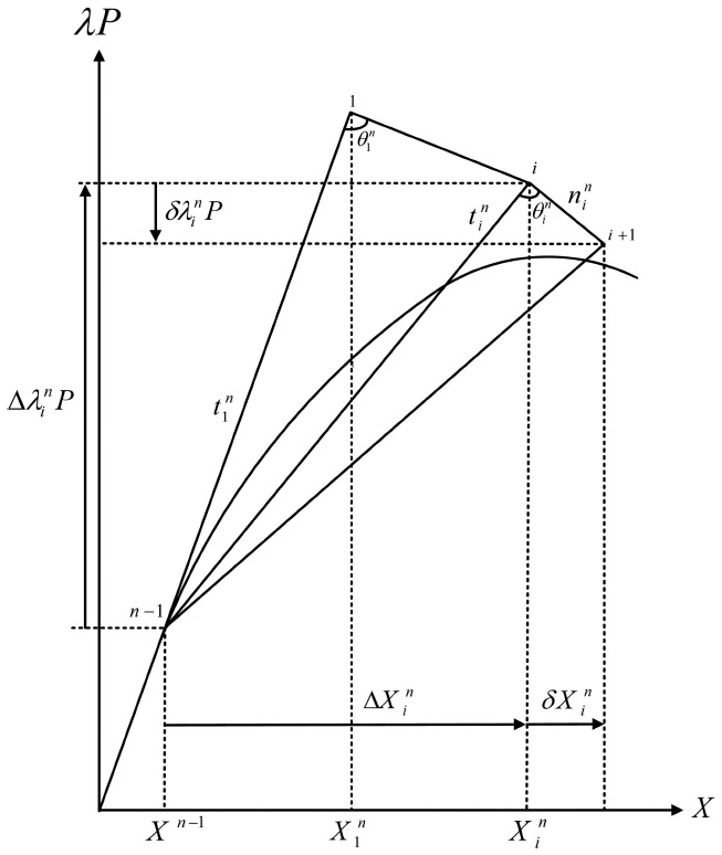
Figure 3 The general procedure of optimized updated normal plane scheme.

According to the recent equation, the inner product of the vectors ${\overrightarrow{t}}_i^n$ and ${\overrightarrow{n}}_i^n$, constitutes an objective function which has two variables. To achieve the constraint equation, this objective function is optimized based on ${\theta }_i^n$ and $\delta {\lambda }_i^n$. At first, function (38) is minimized with respect to the load incremental parameter. Subsequently, the resulted equation has the coming form:

$$\begin{array}{l}(\delta {\lambda }_i^n)[{(\Delta x_i^{n^T}\delta {\widehat{x}}_i^n+\Delta {\lambda }_i^n{P}^{T}P)}^2-{\mathit{Cos}}^2{\theta }_i^n(\delta {\widehat{x}}_i^{n^T}\delta {\widehat{x}}_i^n+P^{T}P)\hfill \\ (\Delta x_i^{n^T}\Delta x_i^n+{(\Delta {\lambda }_i^n)}^2{P}^{T}P)]\hfill \\ +[(\Delta x_i^{n^T}\delta {\overline{x}}_i^n)(\Delta x_i^{n^T}\delta {\widehat{x}}_i^n+\Delta {\lambda }_i^n{P}^{T}P)\hfill \\ -{\mathit{Cos}}^2{\theta }_i^n(\delta {\overline{x}}_i^{n^T}\delta {\widehat{x}}_i^n)(\Delta x_i^{n^T}\Delta x_i^n+{(\Delta {\lambda }_i^n)}^2{P}^{T}P)]=0\hfill \end{array}$$

(39)

By squaring both sides of the relationship (37), the squared cosine of ${\theta }_i^n$ is defined as follows:

$${\mathit{Cos}}^2{\theta }_i^n=\frac{{[\delta {\lambda }_i^n(\Delta x_i^{n^T}\delta {\widehat{x}}_i^n+\Delta {\lambda }_i^n{P}^{T}P)+\Delta x_i^n\delta {\overline{x}}_i^n]}^2}{\begin{array}{l}[\Delta x_i^{n^T}\Delta x_i^n+{(\Delta {\lambda }_i^n)}^2{P}^{T}P]\hfill \\ [{(\delta {\overline{x}}_i^n+\delta {\lambda }_i^n\delta {\widehat{x}}_i^n)}^T(\delta {\overline{x}}_i^n+\delta {\lambda }_i^n\delta {\widehat{x}}_i^n)+{(\delta {\lambda }_i^n)}^2{P}^{T}P]\hfill \end{array}}$$

(40)

Substituting the current equality into Equation (39) and simplifying the result, lead to the next constraint equation:

$$a{(\delta {\lambda }_i^n)}^2+b(\delta {\lambda }_i^n)+c=0$$

(41)

$$\begin{array}{l}a=-{(\Delta {\lambda }_i^n)}^2\delta {\widehat{x}}_i^{n^T}\delta {\overline{x}}_i^n{P}^{T}P-\Delta {\lambda }_i^n\delta {\widehat{x}}_i^{n^T}\delta {\widehat{x}}_i^n\Delta x_i^{n^T}\delta {\overline{x}}_i^n\hfill \\ +\Delta {\lambda }_i^n\Delta x_i^{n^T}\delta {\overline{x}}_i^n{P}^{T}P+\delta {\widehat{x}}_i^{n^T}\delta {\overline{x}}_i^n\Delta x_i^{n^T}\Delta x_i^n\hfill \end{array}$$

(42)

$$\begin{array}{l}b=-{(\Delta {\lambda }_i^n)}^2\delta {\overline{x}}_i^{n^T}\delta {\overline{x}}_i^n{P}^{T}P-2\Delta {\lambda }_i^n\delta {\widehat{x}}_i^{n^T}\delta {\overline{x}}_i^n\Delta x_i^{n^T}\delta {\overline{x}}_i^n\hfill \\ +\delta {\overline{x}}_i^{n^T}\delta {\overline{x}}_i^n\Delta x_i^{n^T}\Delta x_i^n\hfill \end{array}$$

(43)

$$c=-\Delta {\lambda }_i^n\delta {\overline{x}}_i^{n^T}\delta {\overline{x}}_i^n\Delta x_i^{n^T}\delta {\overline{x}}_i^n$$

(44)

In a similar fashion to the previous formulation, after finding the constant coefficients and solving Equation (41), two responses according to Equation (10) are obtained for $\delta {\lambda }_i^n$.

In the following, the second minimization of the inner product of ${\overrightarrow{t}}_i^n$ and ${\overrightarrow{n}}_i^n$ with respect to angle ${\theta }_i^n$, is formulated:

$$\begin{array}{l}\mathit{Sin}2{\theta }_i^n[\Delta x_i^{n^T}\Delta x_i^n+{(\Delta {\lambda }_i^n)}^2{P}^{T}P]\hfill \\ [{(\delta {\lambda }_i^n)}^2(\delta {\widehat{x}}_i^{n^T}\delta {\widehat{x}}_i^n+P^{T}P)+\delta {\lambda }_i^n(2\delta {\widehat{x}}_i^{n^T}\delta {\overline{x}}_i^n)+(\delta {\overline{x}}_i^{n^T}\delta {\overline{x}}_i^n)]=0\hfill \end{array}$$

(45)

By setting the first term of Equation (45) to zero, orthogonality of the subsequent vectors is proved:

$$\mathit{Sin}2{\theta }_i^n=0\Rightarrow {\theta }_i^n={90}^{\circ }\Rightarrow {\overrightarrow{t}}_i^n\perp {\overrightarrow{n}}_i^n$$

(46)

This is an important outcome which is the same hypothesis used for the updated normal plane method [5]. As a result, the next constraint equality belonged to the mentioned scheme, UNP:

$$\delta {\lambda }_i^n=-\frac{\Delta x_i^{n^T}\delta {\overline{x}}_i^n}{\Delta x_i^{n^T}\delta {\widehat{x}}_i^n+\Delta {\lambda }_i^n{P}^{T}P}$$

(47)

Evidently, the second term of Equation (45) is nonzero. Hence, by setting the last term of this equation to zero, the load incremental parameter can be obtained. This way leads to the same quadratic equation, which is Equation (28) with coefficients (29) to (31).

5 Numerical Results

To evaluate the ability of the proposed approaches, a computer program based on new Equations (21) and (41), and also Equation (6), CAL procedure, is provided by authors. On the other hand, two of the obtained similar constraint relations, the normal plane scheme and the updated normal plane technique, are utilized in this program to compare their results with the outcomes of the suggested schemes. The geometric nonlinear analyses of several frames, trusses, and shell are performed via these strategies. For analyzing these structures, the number of convergence points (N_cp), the number of iterations (Ni), and the total analysis duration (T_a) of the schemes are recorded, which are not usually similar to each other. To demonstrate the differences, the number of iterations and increments of all strategies, and also the analysis duration are presented.

It should be added, an assigned number of iterations is used for each step. In each step, the iterative process continues until the number of iterations exceeds the maximum allowable value or the convergence criterion is fulfilled. Also, the amount of the acceptable residual error in the convergence criterion is usually defined in the range of 10⁻⁵ to 10⁻² [9]. In this paper, the maximum number of iterations and the residual error are 10 and 10⁻⁴, respectively. As a common practice, the length factor of the (n)th increment, L_n, is given by [34]:

$$L_n=\pm L_{n-1}{\left(\frac{J_D}{J_{n-1}}\right)}^{0.5}$$

(48)

In this relation, the length factor in the (n-1)th step is shown by L_n−1. Furthermore, the number of iterations assumed by the analyzer and the number of iterations in the (n-1)th step are denoted by J_D and J_n−1, correspondingly. It should be noted, the length factor has the following sign [41]:

$$\mathit{Sign}(L_n)=\mathit{Sign}(\Delta x_{n-1}^T{S}^{-1}P)$$

(49)

In this equality, Δx_n−1 is the displacement vector of the previous step.

5.1 12-Member Space Truss

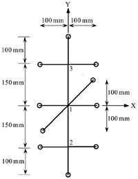
Figure 4 presents a space truss with 13 nodes and nine degrees of freedom. Structural member sizes are shown on this figure. A unit downward vertical load is applied at the center point. Nodes indicated with a circle, are fixed supports at the height of zero, and the other nodes are at 150 mm height. The cross-section area of members, and Young’s modulus of elasticity are 10 mm² and 10³ N/mm², respectively.

Figure 4 12-member space truss.

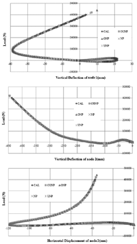
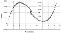
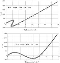
In this paper, the space truss was analyzed 45 times by using ONP, OUNP, CAL, NP, and UNP methods. Note that different initial length factors were utilized. For L₁ = 1, the load-displacement curves of nodes 1 and 2 are illustrated in Figure 5. Based on these diagrams, both novel techniques and also CAL strategy were able to successfully trace the static equilibrium path of the truss with four load and displacement limit points. It should be emphasized that tracing equilibrium path by NP method returned to itself after the first snap-through branch. Furthermore, analyzing with UNP procedure was stopped while reaching to the initial limit point.

By considering the length factor influence of the predictor step, the space truss was analyzed with the different values for the initial length factor. The total number of increments and iterations required for the analysis of this structure are listed in Table 1. According to the results, the optimized normal plane scheme and the optimized updated normal plane technique analyzed successfully 12-member truss with the minimum number of increments and iterations compared to the other methods. It should be noted that these numbers are almost constant and have a slight dependency on the initial length factor for the proposed tactics. Based on the obtained results, CAL strategy needed more iterations and increments for a full assessment of the structural behavior. By comparing the outcomes of the new methods with the other three procedures, the mentioned differences increased for the lower values of L₁. For instance, the CPU time of CAL procedure is several hundred times of ONP and OUNP algorithms if L₁ = 0.01 is applied.

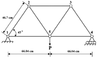
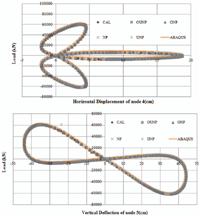
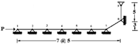
5.2 Seven-Member Truss

Figure 6 illustrates this structure, which has seven degrees of freedom. A concentrated load is applied to the middle of this truss. The cross-section areas of the horizontal members are 54.85 cm², and for the others are 51.65 cm². Moreover, the elasticity modulus of all members is 6889.4 kN/cm². Previously, this truss was analyzed for investigating the elastic buckling of the members [42]. Furthermore, it was employed to verify the ability of the higher-order stiffness matrix in predicting the behavior of structures [35].

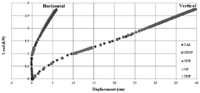
The purpose was to reach the static equilibrium paths for nodes 4 and 5 in the horizontal and vertical direction, correspondingly. The geometric nonlinear analysis of this truss was performed by employing the novel approaches, NP, UNP, and CAL methods. It should be added that this structure was analyzed 30 times. The outputs for the initial length factor equal to 0.5, are shown in Figure 7. Due to the complex structural behavior, the static equilibrium paths of this truss include several snap-through and snap-back regions. However, the techniques of authors, and also the cylindrical arc length tactic could successfully pass all these limit points. Note that the other two algorithms failed in passing the limit points. Besides, to evaluate the accuracy of new methods, seven-member truss was analyzed via Abaqus software by using wire element and static analysis. Figure 7 presents the obtained results, which are consistent with Abaqus outputs.

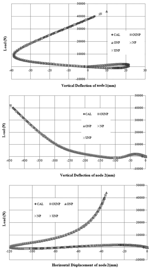
Figure 5 The static equilibrium paths of 12-member space truss.

Table 1 Comparison of the methods utilized for analyzing 12-member space truss

	L1 = 1		L1 = 0.1		L1 = 0.01
Method	Ncp	Ni	Ncp	Ni	Ncp	Ni	Ta (s)
ONP	118	342	126	354	121	329	0.40
OUNP	122	354	129	364	138	386	0.55
CAL	723	2167	7222	21657	72217	216635	70.85
NP	Returns to itself after the first limit point		222	648	Returns to itself after the second load limit point
UNP	Up to the first limit point		Returns to itself after the first limit point		Up to the second load limit point

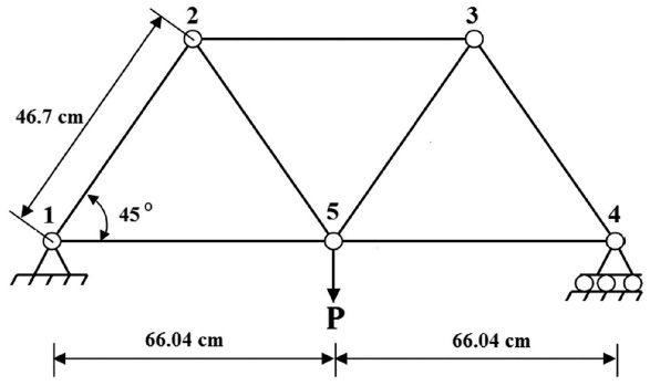
Figure 6 Seven-member truss.

In Table 2, all obtained results with three different values of L₁ are listed. Based on these outcomes, the first suggested technique could accomplish the load-displacement curve with the minimum number of increments and iterations. In other words, the optimized normal plane algorithm was the fastest method to trace the static equilibrium path of this truss for each initial length factor. The optimized updated normal plane scheme with the same characteristics had the next rank. On the contrary, CAL tactic stayed in the third place with the highest number of increments and iterations. Emphasize that for CAL algorithm, these numbers increased greatly while the value of L₁ was reduced. In addition, it was found that the reduction of the initial length factor was ineffective on the performance of the normal plane method and its updated one. However, these two techniques were not able to pass the limit branch of the equilibrium path of this 2D truss.

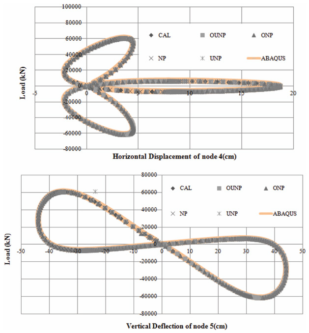
Figure 7 The static equilibrium paths of seven-member truss.

Table 2 Comparison of the methods utilized for analyzing seven-member truss

	Method
	ONP		OUNP		CAL		NP	UNP
L1	Ncp	Ni	Ncp	Ni	Ncp	Ni	Tracing Situation	Tracing Situation
0.01	178	518	176	515	30560	30959	Up to the first load limit point	Up to the first load limit point
0.1	166	490	185	549	3055	5298	Jumps to the third limit point and returns to itself	Up to the third limit point
0.5	145	431	187	565	611	1222	Up to the third limit point	Up to the last limit point

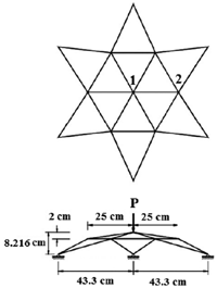
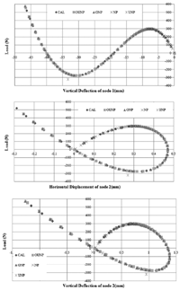
5.3 Star-Shaped Dome Truss

In Figure 8, the plan and view of a 24-member truss are indicated. The elasticity modulus of the members and cross-section area are 3000 N/mm² and 317 mm², respectively. A concentrated unit load is applied to the tip of the truss. This three-dimensional structure has been frequently considered for the nonlinear analysis by other researchers. For example, this benchmark problem was utilized to assess the effect of buckling on the global instability of the truss [43], verify several orthogonal approaches [44], investigate the post buckling behavior of the truss under thermal load [45], and evaluate the capability of the dynamic relaxation scheme [20, 46]. Herein, this space structure was analyzed via the proposed techniques, NP, UNP, and CAL methods.

Figure 9 shows the load-displacement path of nodes 1 and 2 with a unit initial length factor. These curves illustrate the snap-through behavior at these nodes. While the snap-back branch exists at the equilibrium path of node 2. Evidently, the normal plane method could not pass the first load limit point of both nodes and returned to itself. Whereas, the procedures of authors and the cylindrical arc length technique traced the static equilibrium paths completely. These strategies reached the responses compatible with those of the other researches, which is the beginning of the inelastic post buckling of this benchmark structure after accomplishment the load level of 300 N [43]. The updated normal plane scheme finished this analysis by jumping from the second load limit point of the diagrams related to node 2.

The main solution parameters of the suggested algorithms, NP, UNP, and CAL techniques are arranged in Table 3. To reach an actual conclusion, the star truss was analyzed 45 times by using these five methods and different values for L₁. Based on the presented results, the optimized normal plane strategy analyzed star-shaped dome truss with the highest speed, 45–62 increments and 137–166 iterations for three amounts of L₁. The ranges of the increment and iteration numbers were much wider for the cylindrical arc length algorithm, which indicates this strategy greatly depends on the input values. With the numbers close to ONP method, OUNP scheme traced successfully these complex load-displacement curves. The updated normal plane procedure could not pass the load limit points by using decreased initial length factors. On the other hand, the reduction of L₁ had a negative effect on the performance of UNP method. It should be added that this process did not change the ability of NP technique.

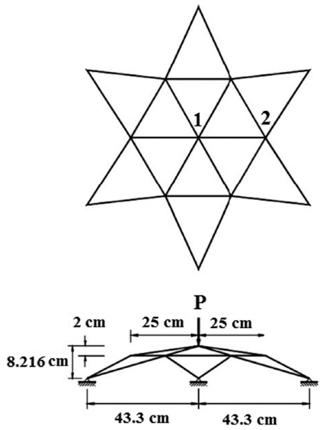
Figure 8 Star-shaped dome truss.

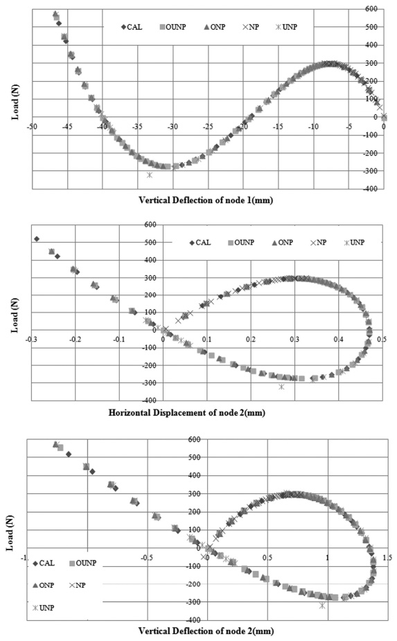
Figure 9 The static equilibrium paths of star-shaped dome truss.

Table 3 Comparison of the methods utilized for analyzing star-shaped dome truss

	Method
	ONP		OUNP		CAL		NP	UNP
L1	Ncp	Ni	Ncp	Ni	Ncp	Ni	Tracing Situation	Ncp	Ni
0.01	62	166	64	174	4816	14437		Up to the first load limit point
0.1	59	168	63	181	482	1442	Returns to itself after the first load limit point	Up to the second load limit point
1	45	137	51	159	49	146		42	144

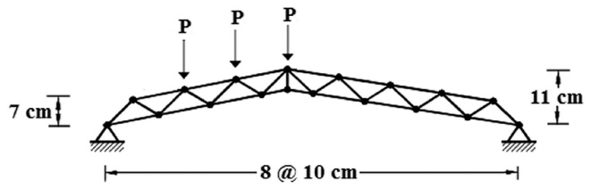
Figure 10 Arch shape truss.

5.4 Arch Shape Truss

In Figure 10, an 18-node two-dimensional truss is illustrated. It has 32 degrees of freedom. Due to the asymmetry of geometry and loading, the behavior of this structure is extremely nonlinear. Previously, researchers analyzed this 33-member truss by using Newton-Raphson [47], the updated normal plane [48], and the zero residual area methods [9]. The cross-section area of all members is 3 cm², and their elasticity modulus is 3 × 10⁶ kN/cm². It should be added that three concentrated vertical loads with the value of 1 kN are applied to this truss.

This example aimed to trace the load-deflection curve of the highest structural node. Figure 11 demonstrates the static equilibrium paths with L₁ = 1. It is obvious that the suggested approaches and CAL method traced the equilibrium path including the snap-back and snap-through branches. On the contrary, the normal plane scheme and the updated one were not able to pass the load limit point.

According to Table 4, the total duration of analysis by CAL technique was minimum for unit initial length factor. However, the CPU time increased extremely while the L₁ value entered lesser. It should be mentioned, the analysis duration related to CAL tactic was 13.45 second for L₁ = 0.01. The T_a parameter of the suggested algorithms was almost constant as the initial length factor was changed. In other words, ONP and OUNP strategies analyzed arch shape truss in the range of 0.5 to 0.8 second.

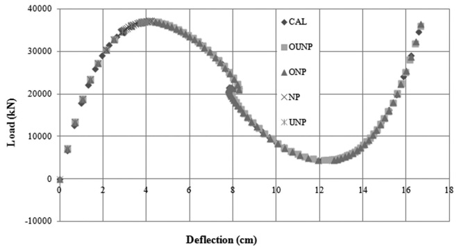
Figure 11 The static equilibrium path of arch shape truss.

Table 4 Comparison of the methods utilized for analyzing arch shape truss

Method	L1	Ta (Second)	L1	Ta (Second)	L1	Ta (Second)
ONP		0.57		0.77		0.69
OUNP		0.58		0.78		0.82
CAL		0.55		2.36		13.45
NP	1		0.1	Jumps from snap-back point to end of the path	0.01
UNP		Up to the first load limit point		Jumps from the first snap-through point to end of the path		Returns to itself after the first limit point

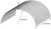
5.5 Semi-Cylindrical Shell

Figure 12 shows a semi-cylindrical shell with 3 mm thickness subjected to a concentrated load in the middle of the free-hanging circumferential periphery. The other curved edge and longitudinal boundaries are fully clamped. Considering the symmetry, it is only needed to analyze half of the shell. Sze and Zheng [49], and also Sze et al. [50] investigated the behavior of this 3D structure with different numbers of meshes. In the following research, 480 triangular meshes used for the analyses. Furthermore, Young’s modulus is taken as E = 2068.5 kN/cm², and Poison’s ratio as ν = 0.3.

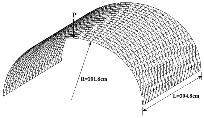
Figure 12 Semi-cylindrical shell.

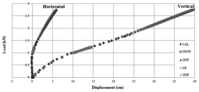
Figure 13 The static equilibrium paths of semi-cylindrical shell.

Figure 13 illustrates equilibrium paths of the loaded point in the horizontal and vertical directions. It should be remembered that NP and UNP techniques only traced the initial part and middle part of the load-displacement curves, respectively. Whereas, the first proposed method analyzed perfectly this benchmark structure with the least time. The number of increments and iterations of ONP approach was 177 and 1237, correspondingly. Furthermore, the second novel scheme required 205 increments and 2872 iterations for tracing the equilibrium paths of semi-cylindrical shell. It should be noted that the analysis duration by CAL tactic was maximum.

5.6 Bridge Truss

As it is demonstrated in Figure 14, this plane truss has nine nodes. All the structural properties of this benchmark problem are assumed to be dimensionless [47, 51]. This truss is under a lateral force that equals to 100. Moreover, the axial stiffness of members, EA, is 3 × 10⁵.

To obtain the equilibrium paths of nodes 1 and 7, this plane truss was examined via novel constraints, UNP, NP and CAL methods. Figure 15 reveals the results of these analyses. The equilibrium path of node 1 indicates snap-back behavior [9]. However, the load-displacement curve of node 7 has snap-through branches. It is obvious that the analyses were completed without any difficulty by using the presented optimized tactics, and also CAL procedure for both nodes of bridge truss. While NP and UNP schemes failed at crossing the second load limit point.

In addition, the total number of increments and iterations of analysis with new methods and the cylindrical arc length technique are shown in Table 5. The results of 40 times analyses with different L₁ amounts indicate that ONP tactic always traced the equilibrium paths of this structure with the least numbers of increments and iterations. The other novel technique achieved the numbers close to ONP method. As it is shown in Table 5, the cylindrical arc length strategy analyzed this eight-bar truss by further increments and iterations [9]. However, NP scheme was not able to pass the second load limit point of the related static equilibrium curves, even by reducing initial length factors. It should be added that decreasing the initial length factor reduced the ability to trace equilibrium path for the updated normal plane method. In other words, end point of the static equilibrium curves were transmitted to the first load limit point by utilizing UNP scheme, while L₁ decreased. According to these results, the procedures of authors worked more quickly than CAL, NP, and UNP techniques. It should be emphasized that NP and UNP schemes could not analyze this benchmark structure completely. As a result, they do not have any value in Table 5.

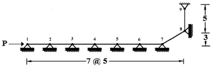
Figure 14 Bridge truss.

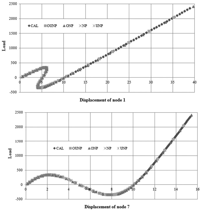
Figure 15 The static equilibrium paths of bridge truss.

Table 5 Comparison of the methods utilized for analyzing bridge truss

	Method
	ONP		OUNP		CAL		UNP
L1	Ncp	Ni	Ncp	Ni	Ncp	Ni	Tracing Situation
0.001	68	168	68	168	81977	81997	Up to the first limit point
0.01	60	151	60	153	8198	8407
0.1	56	148	59	158	820	1126	Up to the second load limit point
1	34	91	47	134	82	182	Returns to itself after the second load limit point

6 Conclusion

In this paper, the static equilibrium paths of various structures were obtained by the optimization schemes. By minimizing the objective functions, resulted from the inner product of vectors, with respect to the load incremental parameter and the angle between vectors, two new formulas were achieved as the constraint equations. The suggested algorithms are able to trace the static load-displacement curves of structures with severe nonlinear behavior, having snap-back and snap-through regions. To prove the capability of these procedures, geometric nonlinear analyses of the several structures were performed. The most outstanding characteristic of the proposed approaches is the rapid convergence rate with high accuracy. In other words, the innovative optimized methods reach the true answers faster than the normal plane, the updated normal plane, and the cylindrical arc length strategies. Furthermore, the accuracy of the new approaches was compared with the results of previous researches.

Note that the speed of these solution techniques is important in the analysis of different structures, when low values for the length factor are utilized. Applying the suggested formulations, the load incremental parameter in each iteration was not influenced by the length factor, significantly. On the contrary, the cylindrical arc length procedure was extremely dependent on the analyzer choice. In other words, the number of increments and iterations, and the analysis duration were related to the magnitude of the length factor specified by the analyzer. In fact, the nonlinear analysis duration increased while the length factor was reduced in the cylindrical arc length strategy. As a result, all the equilibrium paths were traced entirely by the novel optimized schemes. Furthermore, the total number of increments and iterations of the proposed methods was less than those of CAL algorithm. It should be reminded; the length factor did not affect on the analysis duration of ONP and OUNP schemes. It is found that the normal plane, and the updated normal plane techniques could not pass some of the limit points, so these schemes were not able to display the entire static equilibrium path of some structures.

Funding

This study was not funded by any company.

Conflict of Interest

The authors declare that they have no conflict of interest.

Notations

x	displacement vector
λ	load incremental parameter
P	external load vector
Rint(x)	internal load vector
R(x, λ)	residual force vector
$\delta \widehat{x}$	displacement increment due to external load
$\delta \overline{x}$	displacement increment due to residual load
S	tangential stiffness matrix
Ln	length factor
n	increment number
i	iteration number
${\overrightarrow{t}}_{i+1}^n$	vector connecting point (n − 1) to point (i + 1)
a, b, c, α, β, γ	constant coefficients of quadratic equation
Δ	discriminant of second-order equation
${\overrightarrow{n}}_i^n$	vector of iterative points location
${\overrightarrow{t}}_1^n$	tangent vector to previous equilibrium point
θ	angle between $\overrightarrow{n}$ and $\overrightarrow{t}$
Ncp	number of convergence points
Ni	number of iterations
Ta	total analysis duration
JD	number of iterations assumed by analyzer
Jn−1	number of iterations in (n − 1)th step
E	Young’s modulus of elasticity
ν	Poison’s ratio
A	cross-section area

References

[1] Torkamani, M. A. M. and Sonmez, M. 2008. Solution techniques for nonlinear equilibrium equations, Structures Congress: 18th Analysis and Computation Specialty Conference, 1–17.

[2] Chajes, A. and Churchill, J. E. 1987. Nonlinear frame analysis by finite element methods. Journal of Structural Engineering, ASCE, 113(6), 1221–1235.

[3] Batoz, J. L. and Dhatt, G. 1979. Incremental displacement algorithms for nonlinear problems. International Journal for Numerical Methods in Engineering, 14(8), 1262–1266.

[4] Riks, E. 1979. An incremental approach to the solution of snapping and buckling problems. International Journal of Solids and Structures, 15(7), 529–551.

[5] Ramm, E. 1981. Strategies for tracing the nonlinear response near limit points. Nonlinear Finite Element Analysis in Structural Mechanics, Springer, Berlin, Heidelberg, 63–89.

[6] Bergan, P. G. 1980. Solution algorithms for nonlinear structural problems. Computers & Structures, 12(4), 497–509.

[7] Crisfield, M. A. 1981. A fast incremental/iterative solution procedure that handles “snap-through”. Computers & Structures, 13, 55–62.

[8] Chan, S. L. 1988. Geometric and material non-linear analysis of beam-columns and frames using the minimum residual displacement method. International Journal for Numerical Methods in Engineering, 26(12), 2657–2669.

[9] Rezaiee-Pajand, M. and Naserian, R. 2015. Using residual areas for geometrically nonlinear structural analysis. Ocean Engineering, 105(1), 327–335.

[10] Rezaiee-Pajand, M. and Naserian, R. 2018. Geometrical nonlinear analysis based on optimization technique. Applied Mathematical Modelling, 53, 32–48.

[11] Rezaiee-Pajand, M. and Afsharimoghadam, H. 2017. Optimization formulation for nonlinear structural analysis. International Journal of Optimization in Civil Engineering, 7(1), 109–127.

[12] Yang, Y. B. and Shieh, M. S. 1990. Solution method for nonlinear problems with multiple critical points. AIAA Journal, 28(12), 2110–2116.

[13] Cardoso, E. L. and Fonseca, J. S. O. 2007. The GDC method as an orthogonal arc-length method. Communications in Numerical Methods in Engineering, 23(4), 263–271.

[14] Leon, S. E., Lages, E. N., de Araújo, C. N. and Paulino, G. H. 2014. On the effect of constraint parameters on the generalized displacement control method. Mechanics Research Communications, 56, 123–129.

[15] Allgower, E. L. and Georg, K. 1980. Homotopy methods for approximating several solutions to nonlinear systems of equations. Numerical Solution of Highly Nonlinear Problems, W. Forster ed., North-Holland, 253–270.

[16] Saffari, H., Fadaee, M. J. and Tabatabaei, R. 2008. Nonlinear analysis of space trusses using modified normal flow algorithm. Journal of Structural Engineering, ASCE, 134(6), 998–1005.

[17] Rezaei-Pazhand, M. and Alamatian, J. 2005. Superior time step for large deformation analysis by Dynamic Relaxation method. Modares Technical and Engineering, 19, 61–74.

[18] Rezaee Pajand, M. and Taghavian Hakkak, M. 2006. Nonlinear analysis of truss structures using dynamic relaxation. International Journal of Engineering Transactions B: Applications, 19(1), 11–22.

[19] Rezaiee-Pajand, M. and Alamatian, J. 2008. Nonlinear dynamic analysis by dynamic relaxation method. Structural Engineering and Mechanics, 28(5), 549–570.

[20] Rezaiee-Pajand, M. and Alamatian, J. 2011. Automatic DR structural analysis of snap-through and snap-back using optimized load increments. Journal of Structural Engineering, ASCE, 137(1), 109–116.

[21] Rezaiee-Pajand, M., Sarafrazi, S. R. and Rezaiee, H. 2012. Efficiency of dynamic relaxation methods in nonlinear analysis of truss and frame structures. Computers & Structures, 112–113, 295–310.

[22] Rezaiee-Pajand, M. and Alamatian, J. 2010. The dynamic relaxation method using new formulation for fictitious mass and damping. Structural Engineering and Mechanics, 34(1), 109–133.

[23] Rezaiee-Pajand, M., Kadkhodayan, M., Alamatian, J. and Zhang, L. C. 2011. A new method of fictitious viscous damping determination for the dynamic relaxation method. Computers & Structures, 89(9–10), 783–794.

[24] Rezaiee-Pajand, M. and Rezaee, H. 2014. Fictitious time step for the kinetic dynamic relaxation method. Mechanics of Advanced Materials and Structures, 21(8), 631–644.

[25] Rezaiee-Pajand, M., Kadkhodayan, M. and Alamatian, J. 2012. Timestep selection for dynamic relaxation method. Mechanics Based Design of Structures and Machines, 40(1), 42−72.

[26] Rezaiee-Pajand, M. and Estiri, H. 2016. Mixing dynamic relaxation method with load factor and displacement increments. Computers & Structures, 168, 78–91.

[27] Rezaiee-Pajand, M. and Estiri, H. 2016. Computing the structural buckling limit load by using dynamic relaxation method. International Journal of Non-Linear Mechanics, 81, 245–260.

[28] Rezaiee-Pajand, M. and Estiri, H. 2016. Finding equilibrium paths by minimizing external work in dynamic relaxation method. Applied Mathematical Modelling, 40(23–24), 10300–10322.

[29] Rezaiee-Pajand, M. and Estiri, H. 2018. Comparative analysis of three-dimensional frames by dynamic relaxation methods. Mechanics of Advanced Materials and Structures, 25(6), 451–466.

[30] Saffari, H. and Mansouri, I. 2011. Non-linear analysis of structures using two-point method. International Journal of Non-Linear Mechanics, 46(6), 834–840.

[31] Saffari, H., Mirzai, N. M. and Mansouri, I. 2012. An accelerated incremental algorithm to trace the nonlinear equilibrium path of structures. Latin American Journal of Solids and Structures, 9(4), 425–442.

[32] Ritto-Corrêa, M. and Camotim, D. 2008. On the arc-length and other quadratic control methods: Established, less known and new implementation procedures. Computers & Structures, 86(11–12), 1353–1368.

[33] Leon, S. E., Paulino, G. H., Pereira, A., Menezes, I. F. M. and Lages, E. N. 2011. A unified library of nonlinear solution schemes. Applied Mechanics Reviews, 64(4), 040803-1–26.

[34] Rezaiee-Pajand, M., Ghalishooyan, M. and Salehi-Ahmadabad, M. 2013. Comprehensive evaluation of structural geometrical nonlinear solution techniques Part I: Formulation and characteristics of the methods. Structural Engineering and Mechanics, 48(6), 849–878.

[35] Torkamani, M. A. M. and Shieh, J. H. 2011. Higher-order stiffness matrices in nonlinear finite element analysis of plane truss structures. Engineering Structures, 33(12), 3516–3526.

[36] Rezaiee-Pajand, M. and Naserian, R. 2016. Using more accurate strain for three-dimensional truss analysis. Asian Journal of Civil Engineering, 17(1), 107–126.

[37] Rezaiee-Pajand, M. and Naserian, R. 2017. Nonlinear frame analysis by minimization technique. International Journal of Optimization in Civil Engineering, 7(2), 291–318.

[38] Rezaiee-Pajand, M. and Afsharimoghadam, H. 2018. An incremental iterative solution procedure without predictor step. European Journal of Computational Mechanics, 27(1), 58–87.

[39] Rezaiee-Pajand, M., Naserian, R. and Afsharimoghadam, H. 2019. Geometrical nonlinear analysis of structures using residual variables. Mechanics Based Design of Structures and Machines, 47(2), 215–233.

[40] Kweon, J. H. and Hong, C. S. 1994. An improved arc-length method for postbuckling analysis of composite cylindrical panels. Computers & Structures, 53(3), 541–549.

[41] Feng, Y. T., Periać, D. and Owen, D. R. J. 1996. A new criterion for determination of initial loading parameter in arc-length methods. Computers & Structures, 58(3), 479–485.

[42] Timoshenko, S. P. and Gere, J. M. 1961. Theory of elastic stability. New York: McGraw-Hill, 147–150.

[43] Tanaka, K., Kondoh, K. and Atluri, S. N. 1985. Instability analysis of space trusses using exact tangent-stiffness matrices. Finite Elements in Analysis and Design, 1(4), 291–311.

[44] Rezaiee-Pajand, M., Tatar, M. and Moghaddasie, B. 2009. Some geometrical bases for incremental-iterative methods. International Journal of Engineering Transactions B: Applications, 22(3), 245–256.

[45] Yang, Y. B., Lin, T. J., Leu, L. J. and Huang, C. W. 2008. Inelastic postbuckling response of steel trusses under thermal loadings. Journal of Constructional Steel Research, 64(12), 1394–1407.

[46] Rezaiee-Pajand, M. and Sarafrazi, S. R. 2011. Nonlinear dynamic structural analysis using dynamic relaxation with zero damping. Computers & Structures, 89(13–14), 1274–1285.

[47] Powell, G. and Simons, J. 1981. Improved iteration strategy for nonlinear structures. International Journal for Numerical Methods in Engineering, 17(10), 1455–1467.

[48] Rezaiee-Pajand, M., Ghalishooyan, M. and Salehi-Ahmadabad, M. 2013. Comprehensive evaluation of structural geometrical nonlinear solution techniques Part II: Comparing efficiencies of the methods. Structural Engineering and Mechanics, 48(6), 879–914.

[49] Sze, K. Y. and Zheng, S. J. 1999. A hybrid stress nine-node degenerated shell element for geometric nonlinear analysis. Computational Mechanics, 23(5–6), 448–456.

[50] Sze, K. Y., Liu, X. H. and Lo, S. H. 2004. Popular benchmark problems for geometric nonlinear analysis of shells. Finite Elements in Analysis and Design, 40(11), 1551–1569.

[51] Feenstra, P. H. and Schellekens, J. C. J. 1991. Self-adaptive solution algorithm for a constrained Newton-Raphson method. Technical Report 25.2-91-2-13, Delft University of Technology, Delft, The Netherlands.

Biographies

Mohammad Rezaiee-Pajand received his PhD in Structural Engineering from University of Pittsburgh, Pittsburgh, PA, USA. He is currently a Professor at Ferdowsi University of Mashhad (FUM), Mashhad, Iran. His research interests are: Nonlinear structural analysis, Finite element method, Dynamic relaxation method, Composite structures, Structural vibration, Structural dynamics, Nonlinear solvers, Time integration, Plate and shell, Computational plasticity, Structural optimization, Engineering mathematics and Numerical techniques.

Rahele Naserian received his PhD in Structural Engineering from Ferdowsi University of Mashhad (FUM), Iran. She is currently an Assistant Professor at Toos Institute of Higher Education, Mashhad, Iran. Her research interests are: Nonlinear structural analysis, Finite element method, Composite structures and Experimental and numerical simulation of reinforced concrete structures.

Hossein Afsharimoghadam is a Ph.D. student of Structural Engineering at Ferdowsi University of Mashhad (FUM), Iran. He received his B.Sc. degree in Civil Engineering, and also M.Sc. degree in Structural Engineering from FUM. His research interests are: Nonlinear analysis, Structural optimization, Seismic design and Steel structures.

European Journal of Computational Mechanics, Vol. 28_5, 433–466.
doi: 10.13052/ejcm2642-2085.2853
© 2020 River Publishers

Abstract

1 Introduction

2 Cylindrical Arc Length Technique

3 Optimized Normal Plane Strategy

4 Optimized Updated Normal Plane Strategy

5 Numerical Results

5.1 12-Member Space Truss

5.2 Seven-Member Truss

5.3 Star-Shaped Dome Truss

5.4 Arch Shape Truss

5.5 Semi-Cylindrical Shell

5.6 Bridge Truss

6 Conclusion

Funding

Conflict of Interest

Notations

References

Biographies